

Submitted:
14 December 2023
Posted:
18 December 2023
You are already at the latest version
Abstract
Liquid argon technology is widely used by many previous and current neutrino experiments, and it is also promising for future large-scale neutrino experiments. When detecting neutrinos using liquid argon, many hadrons are involved, which can also interact with argon nuclei. In order to gain a better understanding of detection processes, and to simulate neutrino events, knowledge of hadron-argon cross sections is needed. This paper describes a new procedure, which improves upon the previous work with a multi-dimensional unfolding, to measure hadron-argon cross sections in a liquid argon time projection chamber. Through a simplified version of simulation, we demonstrate the validity of this procedure.
Keywords:
Hadron beam
; liquid argon
; cross section
; slicing method
; multi-dimensional unfolding
1. Introduction
Liquid argon (LAr) technology is widely used by many previous and current neutrino experiments, such as MicroBooNE [1], ArgoNeuT [2], ICARUS [3], and it is also planned to be employed by future experiments such as SBND [4], as well as one of the next-generation large-scale neutrino experiments DUNE [5]. Neutrinos are mostly detected by their interactions with argon nuclei, in which many types of hadrons are involved, including both the knockout of nucleons, and the production of mesons. These neutrino-induced hadrons can also interact with nucleons before they escape the nucleus. This may change the kinematics and types of final-state particles that are detected, which complicates the reconstruction of neutrino interactions. These are known as final-state interaction (FSI) effects. In addition, the propagation and further interactions of these final-state hadrons also need to be simulated properly. Therefore, the knowledge of hadron-argon cross sections is required, which is useful to inform FSI and improve simulations as well as their associated uncertainties.
However, there is little experimental data available on argon, and the predictions are mostly derived by interpolating cross-section results from lighter and heavier nuclei [6], such as carbon, sulfur, and iron, which have more data available [7,8,9,10]. In those experiments, the common setup is to implement a beam of a certain type of hadron of interest, and shoot the beam towards a thin target of the material of interest. The survival rate of the beam hadron after the thin target can be measured and be used to calculate the cross section. The increasing popularity of LAr-based detectors has motivated efforts towards making cross-section measurements on LAr. The LArIAT collaboration proposed the thin-slice method to measure hadron-argon cross section using a LAr time projection chamber (LArTPC) [11], which itself can no longer be considered as a thin target of LAr for hadrons. The precise track reconstruction of LArTPC enables researchers to hypothetically divide the detector into several thin slices, and each slice can be considered as an independent thin-target measurement.
The original method treats the measured cross section in each bin independently, and performs an effective correction in each bin to account for inefficiency and bin migration caused by detector resolution. We keep the essential idea of the thin-slice method, and further develop the method with more rigorous statistical procedures, including using multi-dimensional unfolding to consider the full correlations of different measurements. In this paper, Section 2 shows the derivation of the cross-section formula, and Section 3 describes the slicing method in more details. Section 4 describes the measurement procedures on a simplified simulation sample, where all results are derived using an IPython notebook, referred to as hadron-Ar_XS [12]. Some further discussions on the results as well as summary are given in Section 5.
2. Cross-section formula
The total cross section as a function of the incident particle’s kinetic energy E1 is defined according to
where denotes the particle beam flux, and is the infinitesimal reduction of flux. n is the number density of the target material. By moving , the infinitesimal path length of the particle inside the material, to the right-hand side of Equation 1, and then integrating both sides, we get
where is the path length integral. This assumes the cross section remains constant within the variation of E during its passage of .2 For a certain area and a certain period of time, the number of surviving particles detected is proportional to the outgoing particle flux, and thus we have
We can also define the number of interacting particles as . Therefore, after measuring the number of incident particles and the number of surviving particles, the total cross section can be calculated as
When it comes to the exclusive cross section3, we denote a as the signal interaction, and b as all the other interactions, and thus we have , where is the reduction of flux due to the signal interaction. Also we have . Separating based on the type of interactions into in Equation 4, we get
and in Equation 5 are not separable given the logarithm function at the right-hand side. Only when , which implies that is very small, and the thin-target approximation holds, then we can use the approximation and get
Therefore, we have
which is in fact a direct implication from the definition of exclusive cross-section
However, in the slicing method described in Section 3, in each slice we used to calculate is not necessarily small. Therefore, we seek to get an unbiased cross-section formula without the thin-target approximation. From Equation 1 and 8, we have
For a finite , we can estimate this relationship as
where is the effective mean value for the cross section within the variation of E during the passage of .4 Therefore, combining with Equation 4, we have the expression for any channel a as
Because we can never measure in an infinitely small E bin, we will express as in the following sections. In the thin-target approximation, , Equation 11 can be approximated to Equation 7.
3. Slicing method
A LArTPC cannot be seen as a thin target in terms of hadrons, whose mean free path in LAr is on the order of 10 to 100 cm. However, thanks to its high-resolution track reconstruction ability, the LArIAT collaboration proposed the thin-slice method [11], where they hypothetically divide the detector into several slices along the hadron beam direction. Each slice is viewed as a thin target, with a width of several millimeters based on the spacing of the sensing wires. When detecting tracks in the TPC, each slice serves as an independent thin-target experiment. By detecting where the track ends, we know where the interaction happens, and thus fill in the corresponding energy bins of and , which are used to calculate the cross section. The final results are rebinned to wider energy bins such as 50 MeV in order to gain statistics.
Based on the thin-slice method, Ref [13] based on a study on the ProtoDUNE-SP experiment [14] first proposed the idea of energy-slicing, where each energy bin is directly considered as a slice, since the cross section is measured as a function of the kinetic energy of the incident particle.5 Figure 1 shows an illustration of a LArTPC. A beam hadron is incident from the left side of the detector, and leaves a track inside the detector. The beam hadron track ends at the end vertex, where either an interaction occurs or the hadron comes to rest, potentially producing some daughter particles, which can be used to determine the type of the interaction. The kinetic energy of the beam hadron when it enters the detector is denoted as , which is known from beam and it approximately follows a Gaussian distribution given the momentum spread. The kinetic energy of the beam hadron at the end vertex is denoted as . Given these two energies, the track can be divided into several slices based on the pre-defined energy bins. The bin edges are indicated by dark red bars in Figure 1, where the last bar is dashed because the beam hadron does not reach that energy. As shown in Figure 1, the first complete slice is referred to as the initial slice; the slice which has the end vertex is referred to as the end slice. If the interaction occurring at the end vertex is a signal interaction, then the end slice is also referred to as the interaction slice.
The piece of track prior to the initial slice is referred to as an incomplete slice, which will not be used. On the contrary, is inside the end slice.
For convenience, we define the slice index from 1 to the number of energy bins N, starting with the highest energy bin. Therefore, for each beam hadron track, there is an initial slice index , an end slice index , as well as an interaction slice index , which is assigned as null if the interaction occurring at the end vertex is not the signal interaction. In addition, if the end vertex is inside the incomplete slice, then the whole track is not usable, and thus the indices for all three slices will be assigned as null. For a sample of events with a beam hadron track in the detector, the distribution of forms the initial histogram , and similarly we have the end histogram and the interaction histogram . We also define the incident histogram , which will later appear in the cross section formula 14. Each bin of counts the number of tracks which reach the energy corresponding to the slice index , and thus we say the tracks are incident to that slice. Note, for , one event is likely to contribute to multiple bins, since a track can be incident to a sequence of slices until it interacts. In the thin-slice method, for each track, we fill into and into , while is filled from to . can also be calculated by the derived and as 6 [13]
The two expressions are equivalent given
which equals the total number of beam hadron events. Given the relationship between the slice index and the energy E by definition, all of these histograms can also be given as energy histograms.
Comparing to Equation 11, replacing with , with , with , and also, with , we derive the cross section for the signal interaction in each energy bin is given by
where is the energy bin width, and is the stopping power of the hadron in LAr. Therefore, for each beam hadron event, three properties are needed, which are , , and whether or not it is the signal interaction, in order to derive the slice index for , , and . This allows us to treat the three indices as a combined 3D variable, and thus enabling the multi-dimensional unfolding discussed in Section 4.3 and Section 4.4.
4. Procedures and results
4.1. Simulations
All results presented in this paper are obtained from data simulated in hadron-Ar_XS [12]. Although this paper focuses on the method to calculate the cross section, it is worth describing how the simulation is done. Smooth and positive curves are created to represent the hadron-argon cross sections as functions of the hadron’s kinetic energy E, as shown in Figure 2. The signal cross section is the cross section for an exclusive channel that we want to measure, and other cross sections accounts for all the others. The total cross section is given as .
As described in Section 3, for each beam hadron event, we need its initial kinetic energy , the kinetic energy at the end vertex , as well as the type of interaction occurring at the end vertex, in order to use the slicing method to measure the cross section. Therefore, in our simplified simulation, we only aim to generate these three properties for each event. For , we generate a random value following a Gaussian distribution for each event, in order to mimic the momentum spread. For the latter two, we simulate the hadron’s passage inside LAr with a customized step size .7 This means, in each step, we generate a random indicator and decide whether the signal interaction or other interactions happen. If not, it proceeds to the next step, until the hadron reacts or its kinetic energy reaches zero. Thus, it also includes the simulation of particle energy loss inside LAr. We use the Bethe-Bloch formula [16] to model the mean curve as a function of hadron kinetic energy, and in each step, we generate a random value following a simplified version of the Landau-Vavilov distribution [16] as the value to be used in the step. As a result, the energy loss in each step would be if no interaction occurs. The mean curve used in the simulation and an example distribution derived at MeV where the mean approximates 2.10 MeV/cm are shown in Figure 3.
A simulation sample of 100000 events was generated. In this simplified simulation, each event has only three properties relevant to cross-section calculations, which are , , and a flag indicating the fate of the hadron. The distributions of these three properties for the simulation sample are shown in Figure 4.8
4.2. Extracting the true cross section
From the three properties associated with each event, we use an even binning with MeV9 and obtain the relevant histograms as described in Section 3: as the distribution of , as the distribution of , as the distribution of but only for events having the signal interaction. After that, we calculate using Equation 12. The obtained histograms are shown in Figure 5.
Inserting these histograms into Equation 14, we derive the signal cross section 10, as shown in Figure 6. This cross section is calculated originally using the true values of the three properties of each event, and its consistency with the simulation curve suggests the feasibility of the slicing method. For a quantitative comparison of the extracted cross section from the simulation sample against the input curve, we can calculate given as
where is a vector of the input cross section evaluated at the middle point in each energy bin, and denotes the covariance matrix for the calculated true cross sections . The derivation of is described later in Section 4.3. If the reduced , defined as the value divided by the number of bins , approximates 1, it suggests good consistency of the sample with the curve. In Section 5, toy studies are performed to further validate the slicing method.
4.3. Deriving the statistical uncertainty
In the last subSection 4.2, we described how to extract the true cross section, but not yet how to calculate its statistical uncertainty. In order to do so, we consider the problem in a higher dimensional space. This is because the three histograms , , and directly derived from each event, are not independent of each other. For example, for different values of , the distributions of are supposed to be different. In order to fully consider the correlations among them, we define a combined variable as
Here we assign for events with null value, as described in Section 3, and thus there is one more bin in addition to the number of energy bins for each of , , and .11 This definition can be understood as flattening a 3D array into a 1D array. The distribution of this combined variable is shown in Figure 7. Since we have 20 bins for all , , and , there are bins for . The entry in each bin is derived by counting (weighted) events independently, and thus a (weighted) Poisson error can be assigned as the statistical uncertainty for each bin content.
After that, we follow standard error propagation by constructing Jacobian matrix defined as , where x denotes the original variable and f denotes the variable to be transformed into, and thus the covariance matrix is propagated by . There are three steps to go from the covariance matrix for the combined variable to the covariance matrix for the cross section, which are also described in the caption of Figure 8:
- Firstly, the combined variable is projected back to the three axes, namely , , 12, and the covariance matrix for is derived.
- Secondly, the null value bins with for the three variable are ignored, and calculated by Equation 12 replaces , and the covariance matrix for is derived.
- Thirdly, the cross section is calculated using the three energy histograms by Equation 14, and its covariance matrix can be derived by calculating the derivatives appearing in the Jacobian matrix.
With these covariance matrices, the error bars in Figure 5 and Figure 6 are obtained. Figure 8 shows the correlation matrices for these four stages, allowing better visualization than covariance matrices. As can be seen in Figure 8 (c), the off-diagonal blocks are not empty, which suggests there are correlations among different histograms. In Figure 8 (d), the correlation matrix for is diagonal, which suggests the true cross section in each bin is independent. However, this will not be the case for the measured cross section as shown later in Section 4.5, and thus, considering the problem in a higher dimensional space is necessary for a rigorous uncertainty evaluation. 13
4.4. Measurement effects
In practice, the true values of , , and the type of interaction are unknown, but they need to be measured, which may result in some measurement effects, including the detector resolution and inefficiency when measuring the energy, as well as the mis-identification of the type of interaction. is usually measured with external instruments outside the LArTPC, while is derived from with the reconstructed track information in the LArTPC. We also rely on random variables to model these effects effectively rather than simulating events from the origins of the effects. Firstly, to simulate the selection process, a score is generated for each event. Based on whether the score is larger or smaller than a threshold, the event is kept or rejected. The score is generated following a Gaussian distribution, whose mean parameter depends on the true of the event, in order for the efficiency to be non-uniform as a more general case. Secondly, for all events that pass the selection, two random variables following different Gaussian distributions are generated for each event, denoted as and . is used to imitate the resolution on measuring , while accounts for the resolution effects involved with energy deposition of the reconstructed track. Therefore, we have and 14. Finally, in order to simulate the mis-identification among three type of interactions, or to say event fates, which are "no interaction", "signal interaction", "other interactions", a confusion matrix is defined, where each element indicates the possibility of a true fate being recognized as a measured fate. Random numbers are used in order to decide the measured fate of each event according to the defined confusion matrix. As a result, the simulated measurement effects can be seen in Figure 9.
Therefore, for each event in the simulation sample passing the selection, it has three true properties and three measured properties. With these properties, we are able to determine its index for the combined variable in both the true space and the measured space, and thus we can use the simulation sample to model the response matrix as well as the efficiency plot for , which would later be the inputs for unfolding [17] as well as efficiency correction. Figure 10 shows the distribution of the measured combined variable , calculated also by Equation 16 but using the measured values.
For real data, the true information is not available, and thus we use unfolding together with the efficiency correction to transform from the measured histogram to the estimated true histogram, which is referred to as the unfolded histogram. However, the number of bins for in the order of can go to over a thousand. To unfold a histogram with such a large number of bins can be very time-consuming. Fortunately, in our case, despite the large number of bins, the histogram is usually sparse, with many empty bins.15 Therefore, we delete these empty bins in the histogram and the histogram separately, re-index the remaining bins, and denote the new index as . A map is created between and , and another map is created between and . After that, we build the response matrix as well as the efficiency plot of , as shown in Figure 11.
Denoting the response matrix as , and the efficiency as , we have , where holds for the simulation sample. For a data sample, we first use the map for the measured histogram to derive from . Then we rely on an unfolding algorithm of choice to estimate the unfolding matrix, denoted as 16, and thus the unfolded histogram for data is 17. Finally the map for the true histogram is used to transform back to .18
4.5. Fake date result
A sample of 10000 events are generated using the same procedure as the simulation sample, but its true information is not used in order to mimic the real data. After selection, we have 5000 events in this fake data sample. Figure 12 shows the correlation matrices involved in the error propagation from the measured histograms to the final cross section results. Comparing to Figure 8 when extracting the true cross section, there are two extra steps, which are unfolding and mapping back to .
In Figure 12 (a), the correlation matrix for is diagonal because in each bin the events are counted independently. Figure 12 (b) is the correlation matrix for , which is derived from (a) by the unfolding algorithm of choice. We use the Python version of RooUnfoldBayes [19] as the unfolding algorithm, which employs the d’Agostini method [20]. The unfolding algorithm is treated as a black box in this paper, where we input the measured histograms as well as its covariance matrix, and get the output including the unfolded histograms as well as its covariance matrix.19 We proceed with the number of iterations as 4, which is the only parameter in d’Agostini’s method for unfolding, and it is not optimized in this work. After that, is converted back to under the map created using the measured histograms, and then the following steps are the same with the error propagation of the true cross section as described in Section 4.3. Figure 13 shows the cross section measured using the fake data sample, whose correlation matrix is shown as Figure 12(f). The correlation matrix is not diagonal, which means the measured cross section in each energy bin is correlated, and thus for the final cross section result, we need to present both the central values as well as its covariance matrix. We can also calculate of the measured cross section against the simulation curve by Equation 15, whose value is shown in the legend of Figure 13. The error bars in the lower-energy bins tend to be larger mostly because the statistics is smaller, since most hadrons interact before they reach these low energies. This trend can also be seen in the true cross section in Figure 6 for the same reason.
5. Discussions and summary
In the previous section, we described how to extract the true cross section of the simulation sample, as well as how to measure the cross section of a data sample. is calculated in both cases, which is used to quantify the consistency against the simulation curve. In order to further test the results, we perform toy studies. 400 simulation samples, referred to as toys, each with a sample of 10000 events, are generated in the same way as what is described in Section 4. The true cross section as well as its covariance matrix is calculated in each toy simulation sample. For each cross-section bin, we calculate the pull value of each toy, which is defined as
where is the uncertainty for . In each bin, the pull values are expected to follow a normal distribution. Figure 14 (a) shows the test results, where a Gaussian distribution is fitted on the pull histograms in each cross-section bin as shown as the blue error bars. By visually comparing with the reference lines, we can see they are generally consistent with the expectation that each of them centers at 0 and has a bar length of 1, corresponding to the two parameters in the Gaussian fit. As another test, which takes into account the covariance among cross-section bins, we show in Figure 14 (b) the histogram of calculated according to Equation 15 for each toy. A distribution is fitted on the histogram, whose degree of freedom , as shown in the legend, is consistent with the expectation, which is 18 as the number of cross-section bins. These tests serve as a validation of the slicing method. They also suggests that given the current statistics of events in each toy, the bias caused by the imperfection of the model20 is insignificant.
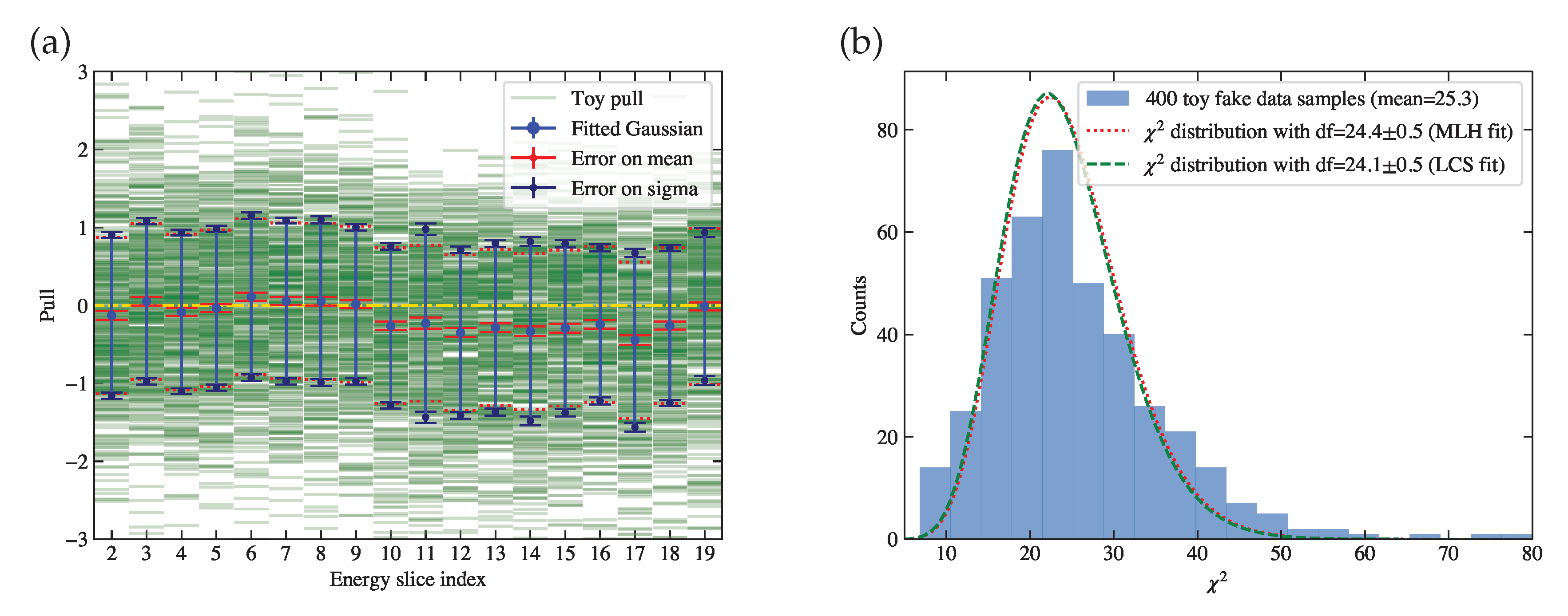
Similarly, we generate 400 toy fake data samples, each with a sample of 10000 events before selection, in order to study the performance of the procedures to measure the cross section. The 400 toy simulation samples used above are combined into a total of 4000000 events, in order to model the response matrix as well as the efficiency plot for each toy fake data sample, and thus we can ignore the statistical uncertainty of the simulation sample. The cross section is measured for each toy fake data sample, and we can also derive the pull distributions in each cross-section bin as well as the histogram of , as shown in Figure 15. In subplot (a), we can see the lengths of blue error bars are generally consistent with 1, but some of their central points show a small bias away from 0. This bias is also referred to as unfolding error. The general unfolding results is effectively applying a re-smearing matrix on the truth information [21]. Treating the re-smeared truth as truth introduces an unfolding error, which can be eliminated by publishing the re-smearing matrix. In addition, the unfolding error tends to be smaller when the regularization becomes weaker with a greater number of iterations. As a result, since we do not include biases, the derived distribution in Figure 15 (b) is larger.
In the fake data toy study, the simulation sample used to model the response matrix and the efficiency plot is consistent with the toy fake data samples, because they are generated in the same way. When it comes to real data, we need to consider the uncertainties caused by the differences between data and simulation, which can be estimated by fluctuating the relevant parameters of the simulation sample. Additional model validation procedure is essential to examine the compatibility between data and simulation to ensure the differences are within the quoted simulation uncertainties.
In summary, a method as well as the corresponding procedures for the hadron-argon cross section measurement in a LArTPC detector is provided in this paper. The method requires the inputs of the initial energy and the energy at the end vertex of the track, as well as whether it is signal interaction occurring at the end vertex. The method shows good statistical performance, with no obvious bias except for that caused by unfolding, and good estimation of statistical uncertainties, as suggested by the toy studies. To apply it to real data, the systematic uncertainties due to the difference between data and simulation should be considered, and the parameters of the unfolding algorithm used should be optimized with further investigations into the trade-off between bias and variance. These features can be added to the IPython notebook hadron-Ar_XS [12], which also has the potential to be extended to more cross-section studies.
Funding
This material is based upon work supported by the National Science Foundation under Grant No. 2209601.
Data Availability Statement
The notebook can be found at Ref [12].
Acknowledgments
This study was initiated from analyzing pion-argon data on the ProtoDUNE-SP experiment [14]. The author would like to thank Edward Blucher and Tingjun Yang for direct discussions on this study, and also would like to thank Jacob Calcutt, Richard Diurba, Stephen Dolan, Elise Hinkle, Thomas Junk, Heng-Ye Liao, Laura Munteanu, Sungbin Oh, Ajib Paudel, Francesco Pietropaolo, Xin Qian, David Schmitz, Francesca Stocker, Leigh Whitehead, Kang Yang, and other collaborators for various useful discussions on the ProtoDUNE-SP data analyses.
References
- Acciarri, R.; others. Design and Construction of the MicroBooNE Detector. JINST 2017, 12, P02017, [arXiv:physics.ins-det/1612.05824]. [Google Scholar] [CrossRef]
- Anderson, C.; others. The ArgoNeuT Detector in the NuMI Low-Energy beam line at Fermilab. JINST 2012, 7, P10019, [arXiv:physics.ins-det/1205.6747]. [Google Scholar] [CrossRef]
- Amerio, S.; others. Design, construction and tests of the ICARUS T600 detector. Nucl. Instrum. Meth. A 2004, 527, 329–410. [Google Scholar] [CrossRef]
- Machado, P.A.; Palamara, O.; Schmitz, D.W. The Short-Baseline Neutrino Program at Fermilab. Ann. Rev. Nucl. Part. Sci. 2019, 69, 363–387, [arXiv:hep-ex/1903.04608]. [Google Scholar] [CrossRef]
- Acciarri, R.; others. Long-Baseline Neutrino Facility (LBNF) and Deep Underground Neutrino Experiment (DUNE): Conceptual Design Report, Volume 1: The LBNF and DUNE Projects 2016. [arXiv:physics.ins-det/1601.05471].
- Dytman, S.; Hayato, Y.; Raboanary, R.; Sobczyk, J.T.; Tena Vidal, J.; Vololoniaina, N. Comparison of validation methods of simulations for final state interactions in hadron production experiments. Phys. Rev. D 2021, 104, 053006, [arXiv:hep-ph/2103.07535]. [Google Scholar] [CrossRef]
- Wilkin, C.; Cox, C.R.; Domingo, J.J.; Gabathuler, K.; Pedroni, E.; Rohlin, J.; Schwaller, P.; Tanner, N.W. A comparison of pi+ and pi- total cross-sections of light nuclei near the 3-3 resonance. Nucl. Phys. B 1973, 62, 61–85. [Google Scholar] [CrossRef]
- Clough, A.S.; others. Pion-Nucleus Total Cross-Sections from 88-MeV to 860-MeV. Nucl. Phys. B 1974, 76, 15–28. [Google Scholar] [CrossRef]
- Carroll, A.S.; Chiang, I.H.; Dover, C.B.; Kycia, T.F.; Li, K.K.; Mazur, P.O.; Michael, D.N.; Mockett, P.M.; Rahm, D.C.; Rubinstein, R. Pion-Nucleus Total Cross-Sections in the (3,3) Resonance Region. Phys. Rev. C 1976, 14, 635–638. [Google Scholar] [CrossRef]
- Ashery, D.; Navon, I.; Azuelos, G.; Walter, H.K.; Pfeiffer, H.J.; Schleputz, F.W. True Absorption and Scattering of Pions on Nuclei. Phys. Rev. C 1981, 23, 2173–2185. [Google Scholar] [CrossRef]
- Gramellini, E.; others. Measurement of the π–Ar total hadronic cross section at the LArIAT experiment. Phys. Rev. D 2022, 106, 052009, [arXiv:hep-ex/2108.00040]. [Google Scholar] [CrossRef]
- Tutorial for the hadron-Ar XS measurement using slicing method. https://github.com/Yinrui-Liu/hadron-Ar_XS. Accessed: 2023-12-1.
- Stocker, F. Measurement of the Pion Absorption Cross-Section with the ProtoDUNE Experiment. PhD thesis, University of Bern, 2021.
- Abi, B.; others. First results on ProtoDUNE-SP liquid argon time projection chamber performance from a beam test at the CERN Neutrino Platform. JINST 2020, 15, P12004, [arXiv:physics.ins-det/2007.06722]. [Google Scholar] [CrossRef]
- Liu, Y. Pion–Argon Inclusive Cross-Section Measurement on ProtoDUNE-SP. Phys. Sci. Forum 2023, 8, 52. [Google Scholar] [CrossRef]
- Workman, R.L.; Others. Review of Particle Physics. PTEP 2022, 2022, 083C01. [Google Scholar] [CrossRef]
- Cowan, G. A survey of unfolding methods for particle physics. Conf. Proc. C 2002, 0203181, 248–257. [Google Scholar]
- CLOPPER, C.J.; PEARSON, E.S. THE USE OF CONFIDENCE OR FIDUCIAL LIMITS ILLUSTRATED IN THE CASE OF THE BINOMIAL. Biometrika 1934, 26, 404–413, [https://academic.oup.com/biomet/article-pdf/26/4/404/823407/26-4-404.pdf]. [Google Scholar] [CrossRef]
- Brenner, L.; Balasubramanian, R.; Burgard, C.; Verkerke, W.; Cowan, G.; Verschuuren, P.; Croft, V. Comparison of unfolding methods using RooFitUnfold. Int. J. Mod. Phys. A 2020, 35, 2050145, [arXiv:physics.data-an/1910.14654]. [Google Scholar] [CrossRef]
- D’Agostini, G. A Multidimensional unfolding method based on Bayes’ theorem. Nucl. Instrum. Meth. A 1995, 362, 487–498. [Google Scholar] [CrossRef]
- Tang, W.; Li, X.; Qian, X.; Wei, H.; Zhang, C. Data Unfolding with Wiener-SVD Method. JINST 2017, 12, P10002, [arXiv:physics.data-an/1705.03568]. [Google Scholar] [CrossRef]
| 1 | For convenience, and are used interchangeably throughout the text. |
| 2 | In reality, indicates an effective mean value for cross section within the variation of E, since there will always be energy loss during the particle’s passage inside the material when we measure the cross section. This also applies to a finite passage length, as discussed in the last paragraph of the section. |
| 3 | Even for the inclusive cross section, there may be reduction of flux due to particle decay. In this case, a denotes the total inelastic interaction, and b denotes particle decay, and thus is considered as an effective cross section. For convenience, we will refer to particle decay also as an "interaction". |
| 4 | |
| 5 | |
| 6 | The calculation enables us to derive using the unfolded histogram given in Section 4.4. This is because after unfolding, the event-wise information is lost and cannot be derived by counting events. In addition, for , it is no longer one entry per track, and thus it would be problematic to unfold the counted directly. |
| 7 | Simulation used in this paper is generated with cm, which should be much smaller than the mean free path of a particle with cross section in the order of 1000 mb. |
| 8 | There could be a fourth property for each event, which is the event weight. To simplify the problem, we assign uniform weights for all samples used in this paper, but the procedures also apply to samples with non-uniform weights. |
| 9 | The binning is not necessary to be even, and it should be decided on a case-by-case basis. |
| 10 | In principle, and can also be derived using the same method. |
| 11 | Considering this null-value bin is because it is possible to be given as a normal bins in the measured histogram described in Section 4.4, and thus it is needed in order to build the response matrix. |
| 12 | This can be done by calculating , , and , where N denotes the bin content for the corresponding . |
| 13 | The matrix may look to be empty because it is sparse and the bins may be too small for readers to visualize its color. Similarly, it happens to Figure 12 (c). |
| 14 |
is derived from the measurement of , so is inherited. |
| 15 | |
| 16 |
does not indicates the inverse of R, which is proven problematic to use, which is described in many references about unfolding, for example, Chapter 9 in Ref [17]. |
| 17 | If in bin i is 0, the value in the bin can be estimated using the simulation sample normalized to data sample directly, because the zero efficiency is usually due to low statistics and it will not change the final result significantly. However, the uncertainty associated with this can be evaluated by fluctuating these bin entries. |
| 18 | It is possible that a bin for is empty in the simulation sample but not empty in the data sample, especially for bins with low statistics. In this case, we can add these non-empty bins in data to the map as well. It is not necessary for the map to be the same for all data samples. |
| 19 | However, because the histogram we unfold is not a smooth physical spectrum, and thus the unfolding algorithms that try to regularize the unfolded result by smoothing may not be applicable. |
| 20 | For example, we considers the cross section calculated to be at the middle point in each energy bin, and we evaluated also at the middle energy value. These may need further corrections if the statistical uncertainty becomes smaller when the sample size is much larger. |
Figure 1.
An illustration of a LArTPC, where a beam hadron is shot into the detector from the left side. More descriptions of the elements in the illustration are provided in the text.
Figure 1.
An illustration of a LArTPC, where a beam hadron is shot into the detector from the left side. More descriptions of the elements in the illustration are provided in the text.
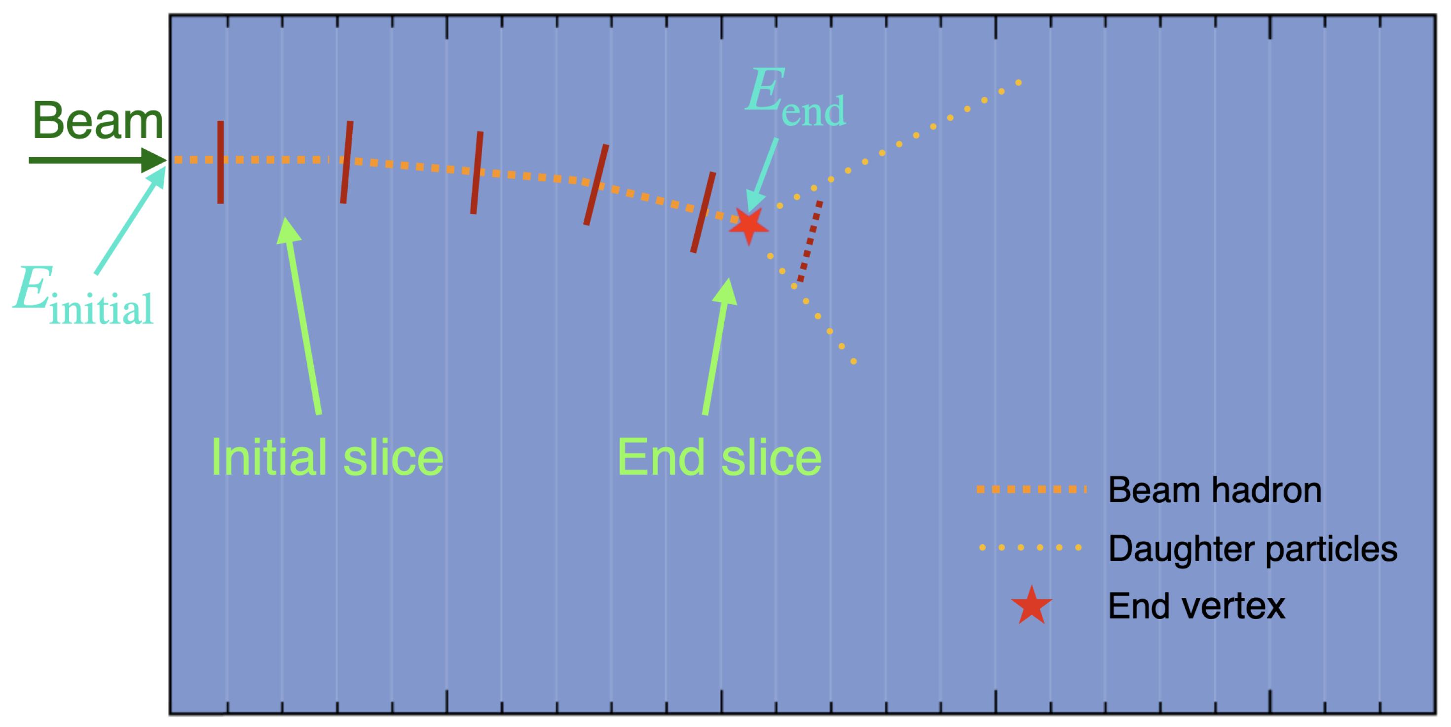
Figure 2.
Cross-section curves based on which the simulation is generated. The total cross section (blue dash-dotted curve) is the sum of the signal cross section (orange solid curve) and the other cross sections (green dashed curve).
Figure 2.
Cross-section curves based on which the simulation is generated. The total cross section (blue dash-dotted curve) is the sum of the signal cross section (orange solid curve) and the other cross sections (green dashed curve).
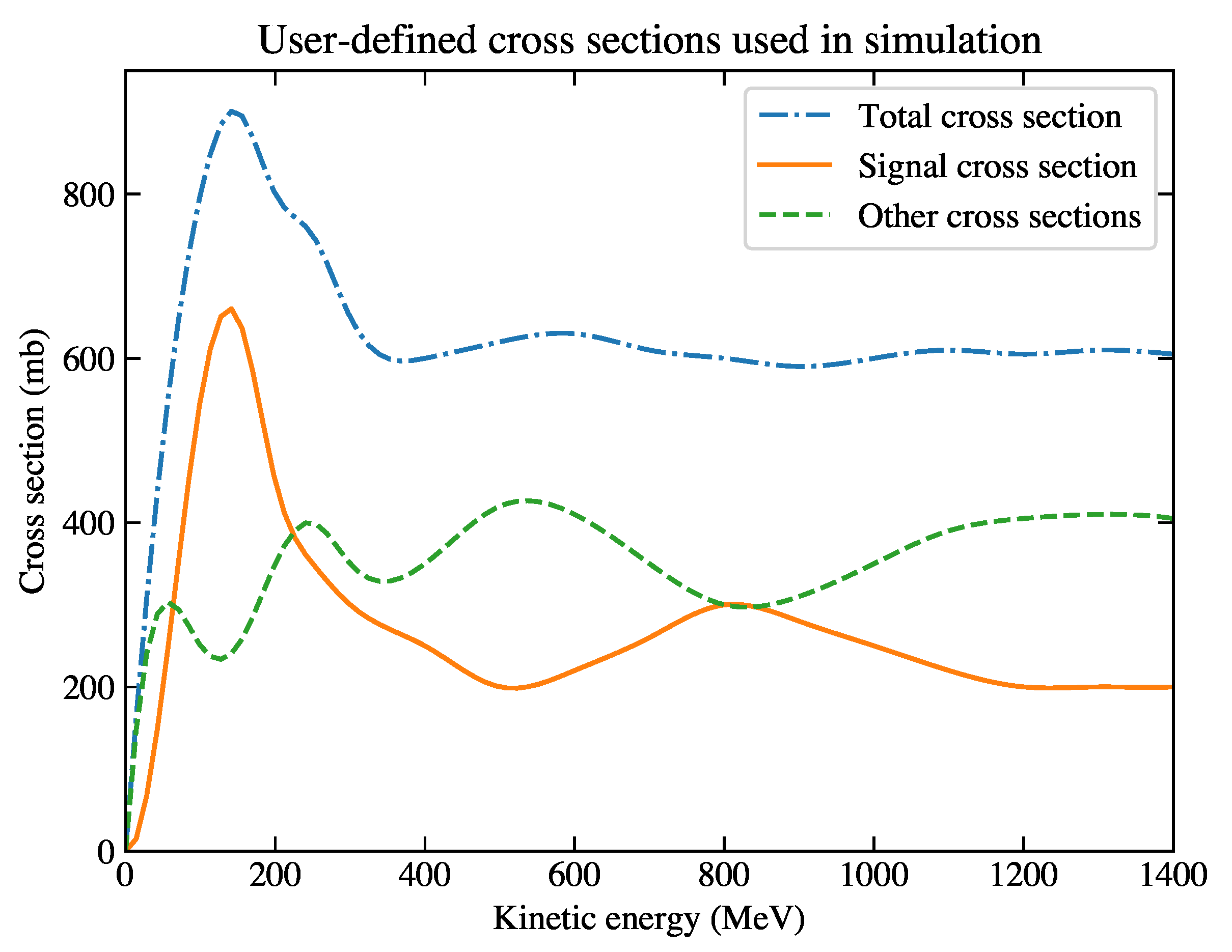
Figure 3.
(a) The mean curve used in the simulation. The dashed vertical line at MeV indicates the case of the example distribution. (b) The example distribution at MeV, where the mean approximates 2.10 MeV/cm.
Figure 3.
(a) The mean curve used in the simulation. The dashed vertical line at MeV indicates the case of the example distribution. (b) The example distribution at MeV, where the mean approximates 2.10 MeV/cm.
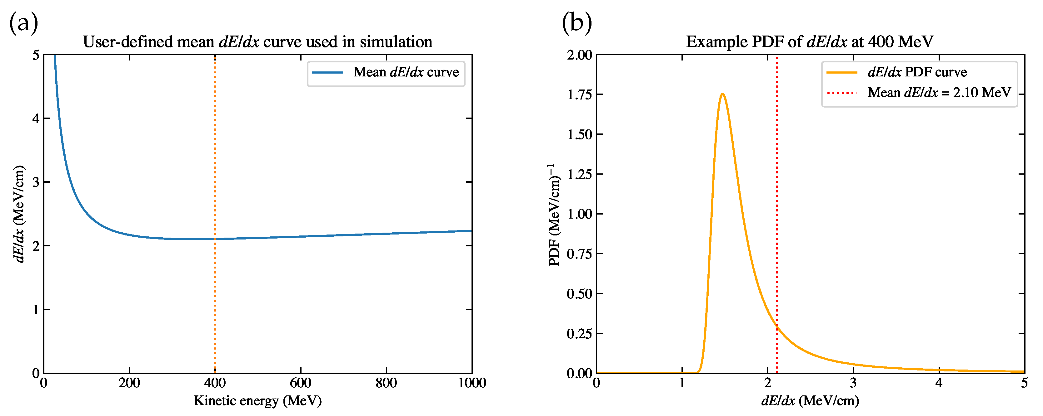
Figure 4.
Of the simulation sample, the distribution of (a) , (b) , (c) the flag indicating the fate of the hadron, either it has no interaction before it comes to rest, or it has signal interaction, or other interactions.
Figure 4.
Of the simulation sample, the distribution of (a) , (b) , (c) the flag indicating the fate of the hadron, either it has no interaction before it comes to rest, or it has signal interaction, or other interactions.
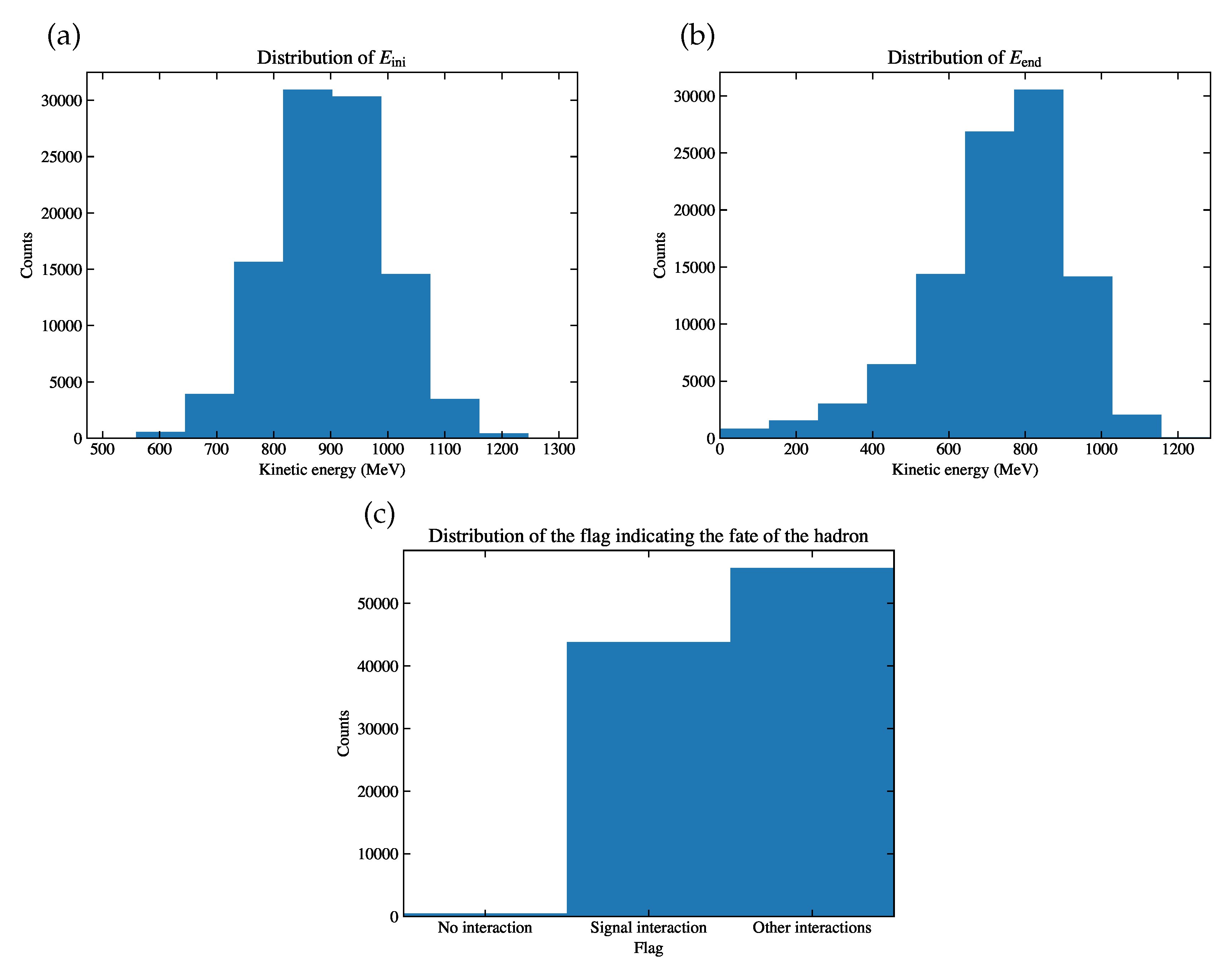
Figure 5.
Energy histograms derived from the simulation sample, (a) , (b) , (c) , (d) . The first and the last energy bins are given as overflows. The derivation of error bars are described later in Section 4.3.
Figure 5.
Energy histograms derived from the simulation sample, (a) , (b) , (c) , (d) . The first and the last energy bins are given as overflows. The derivation of error bars are described later in Section 4.3.
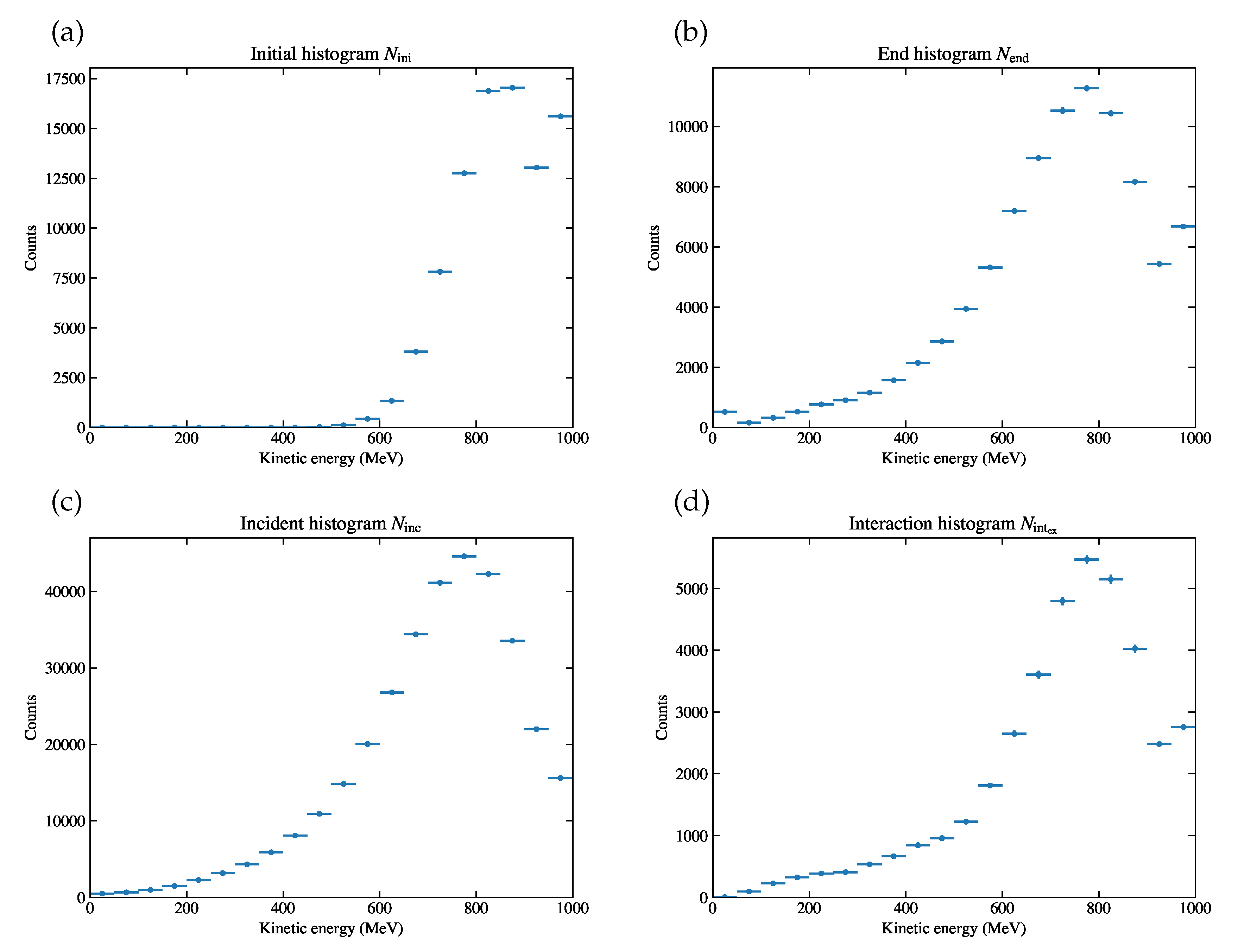
Figure 6.
The cross section extracted using the true information of the simulation sample. The reduced is approximately 1, which suggests good agreement between the sample and the input cross section. The derivation of error bars are described later in Section 4.3.
Figure 6.
The cross section extracted using the true information of the simulation sample. The reduced is approximately 1, which suggests good agreement between the sample and the input cross section. The derivation of error bars are described later in Section 4.3.
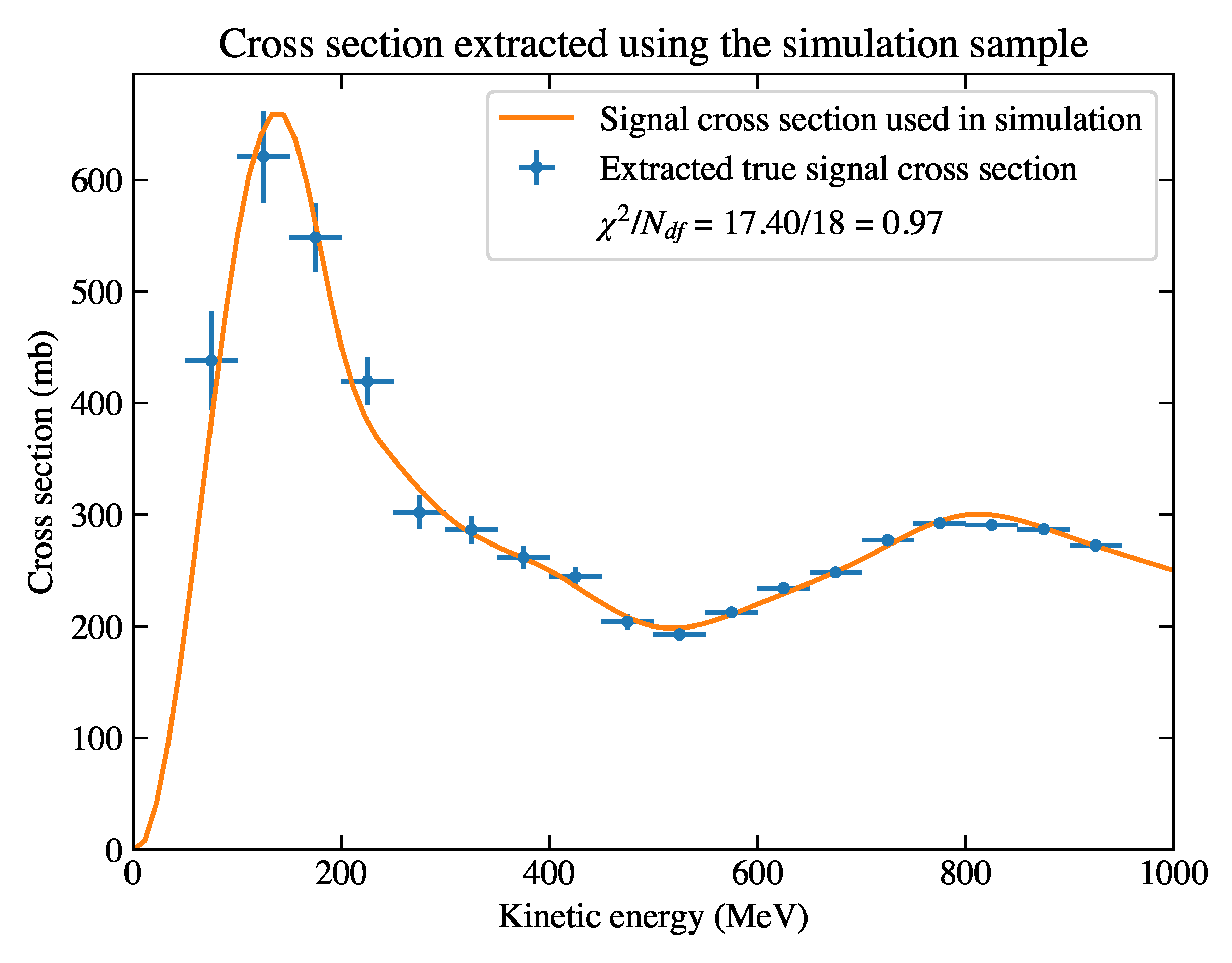
Figure 7.
The distribution of the combined variable of the simulation sample.
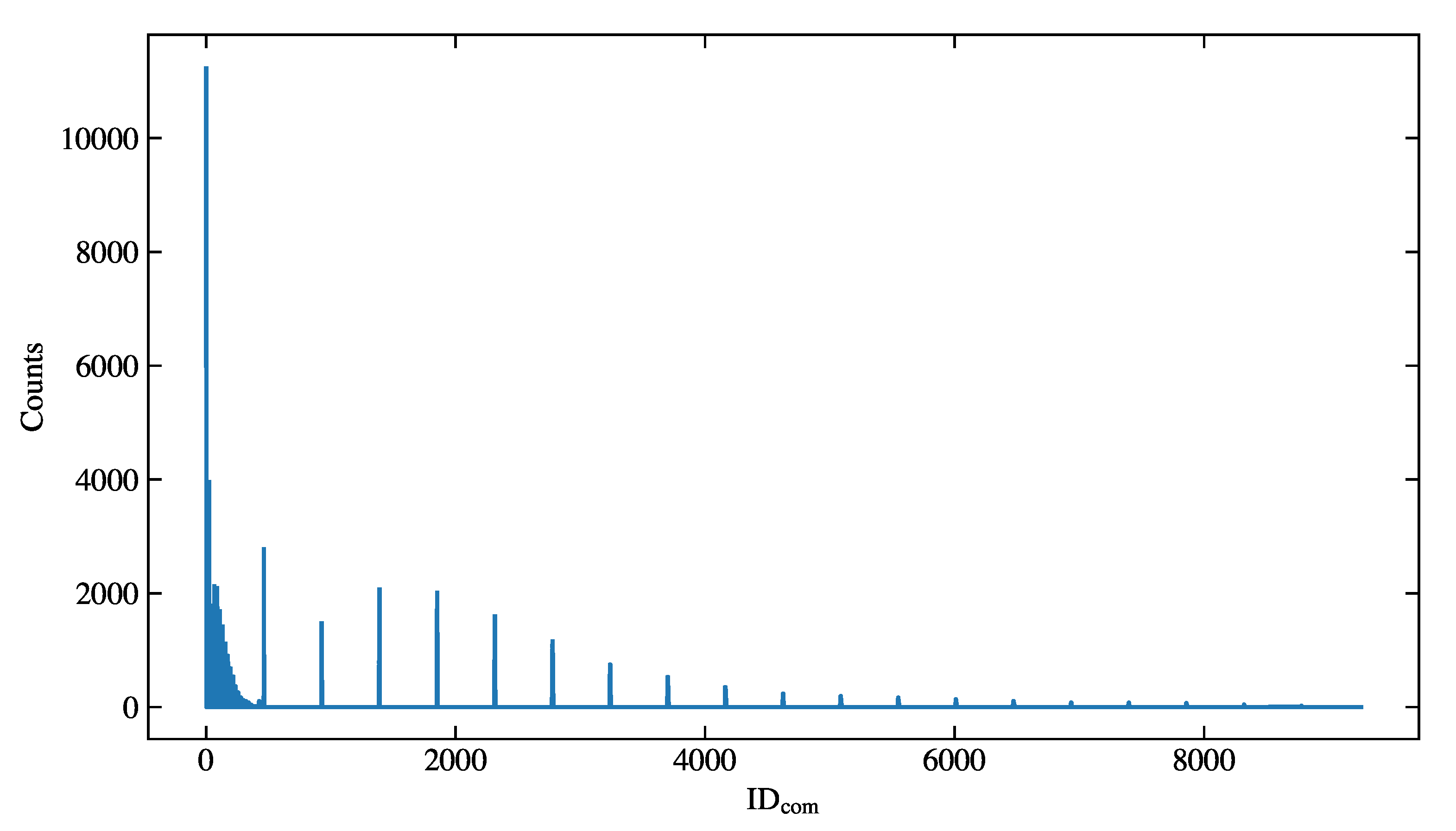
Figure 8.
(a) Correlation matrix for the combined variable , which is diagonal since the entry in each bin is derived by counting independently. (b) Correlation matrix for ; ; , where the first block (bin index 0 to 20) corresponds to , the second block (bin index 21 to 41) corresponds to , and the third block (bin index 42 to 62) corresponds to . (c) Correlation matrix for ; ; , where the first block (bin index 0 to 19) corresponds to , the second block (bin index 20 to 39) corresponds to , and the third block (bin index 40 to 59) corresponds to . (d) Correlation matrix for the extracted cross section , which has 18 bins on each axis without the underflow and the overflow bins.
Figure 8.
(a) Correlation matrix for the combined variable , which is diagonal since the entry in each bin is derived by counting independently. (b) Correlation matrix for ; ; , where the first block (bin index 0 to 20) corresponds to , the second block (bin index 21 to 41) corresponds to , and the third block (bin index 42 to 62) corresponds to . (c) Correlation matrix for ; ; , where the first block (bin index 0 to 19) corresponds to , the second block (bin index 20 to 39) corresponds to , and the third block (bin index 40 to 59) corresponds to . (d) Correlation matrix for the extracted cross section , which has 18 bins on each axis without the underflow and the overflow bins.
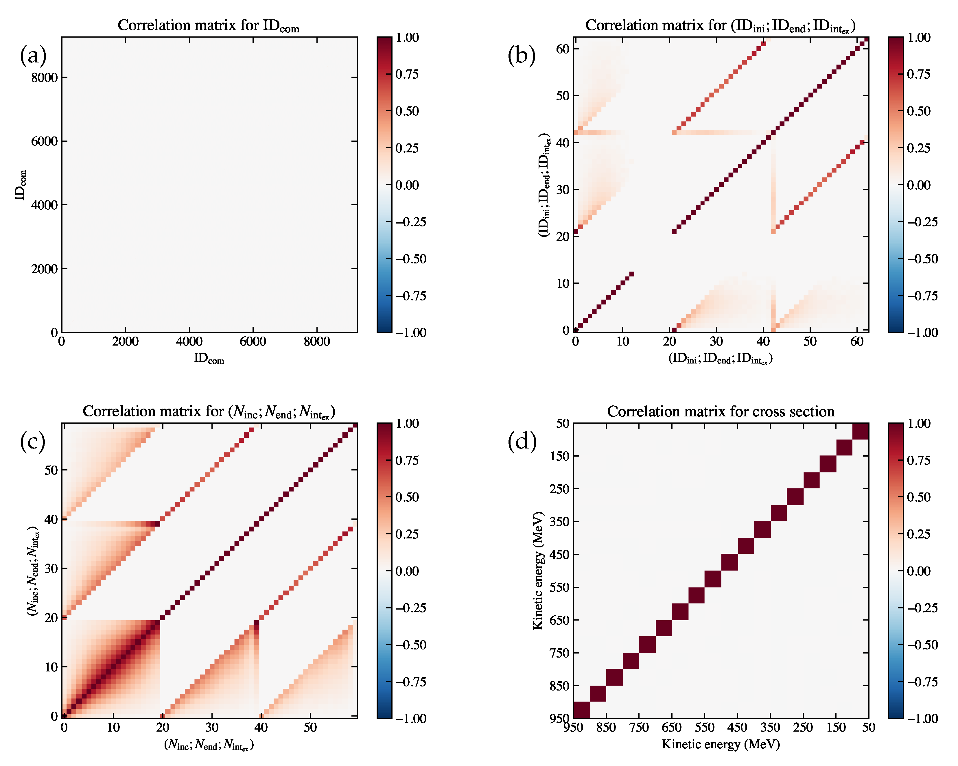
Figure 9.
(a) The distribution of (orange histogram) and (blue histogram) for the simulation sample. (b) The distribution of (orange histogram) and (blue histogram) for the simulation sample. (c) The resulting confusion matrix for event fates of the simulation sample. The horizontal axis indicates the measured fates, and the vertical axis indicates the true fates. The color bar indicates the (weighted) event counts in each bin, which add up to be the event counts passing the selection.
Figure 9.
(a) The distribution of (orange histogram) and (blue histogram) for the simulation sample. (b) The distribution of (orange histogram) and (blue histogram) for the simulation sample. (c) The resulting confusion matrix for event fates of the simulation sample. The horizontal axis indicates the measured fates, and the vertical axis indicates the true fates. The color bar indicates the (weighted) event counts in each bin, which add up to be the event counts passing the selection.
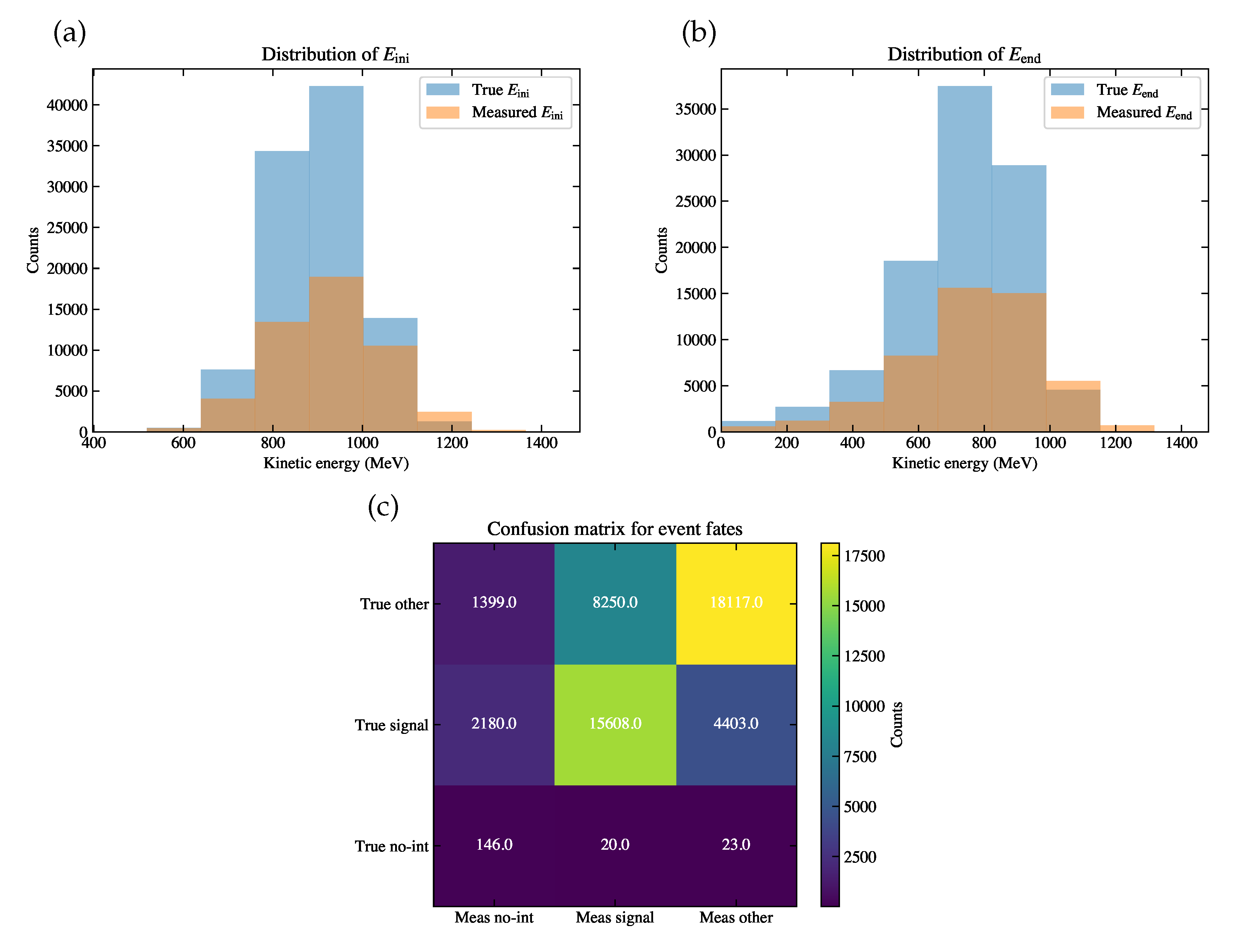
Figure 10.
The distribution of the measured combined variable of the simulation sample.
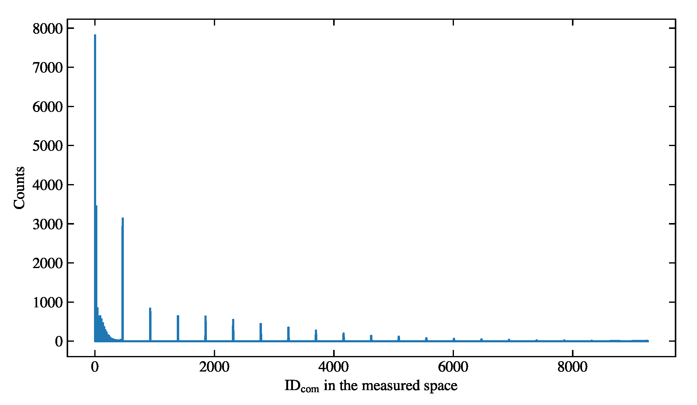
Figure 11.
(a) The response matrix modeled using the simulation sample. The horizontal axis is , and the vertical axis is the true . The color bar indicates the (weighted) event counts in each bin. (b) The efficiency for each bin. The uncertainty for efficiency is calculated according to the Clopper Pearson method [18].
Figure 11.
(a) The response matrix modeled using the simulation sample. The horizontal axis is , and the vertical axis is the true . The color bar indicates the (weighted) event counts in each bin. (b) The efficiency for each bin. The uncertainty for efficiency is calculated according to the Clopper Pearson method [18].
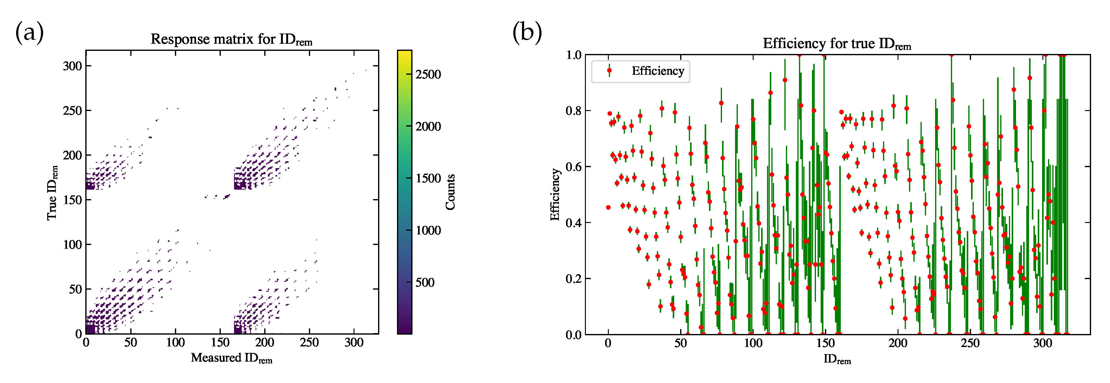
Figure 12.
Correlation matrices for (a) , (b) , (c) , (d) , (e) , (f) the measured cross section , for the fake data sample.
Figure 12.
Correlation matrices for (a) , (b) , (c) , (d) , (e) , (f) the measured cross section , for the fake data sample.
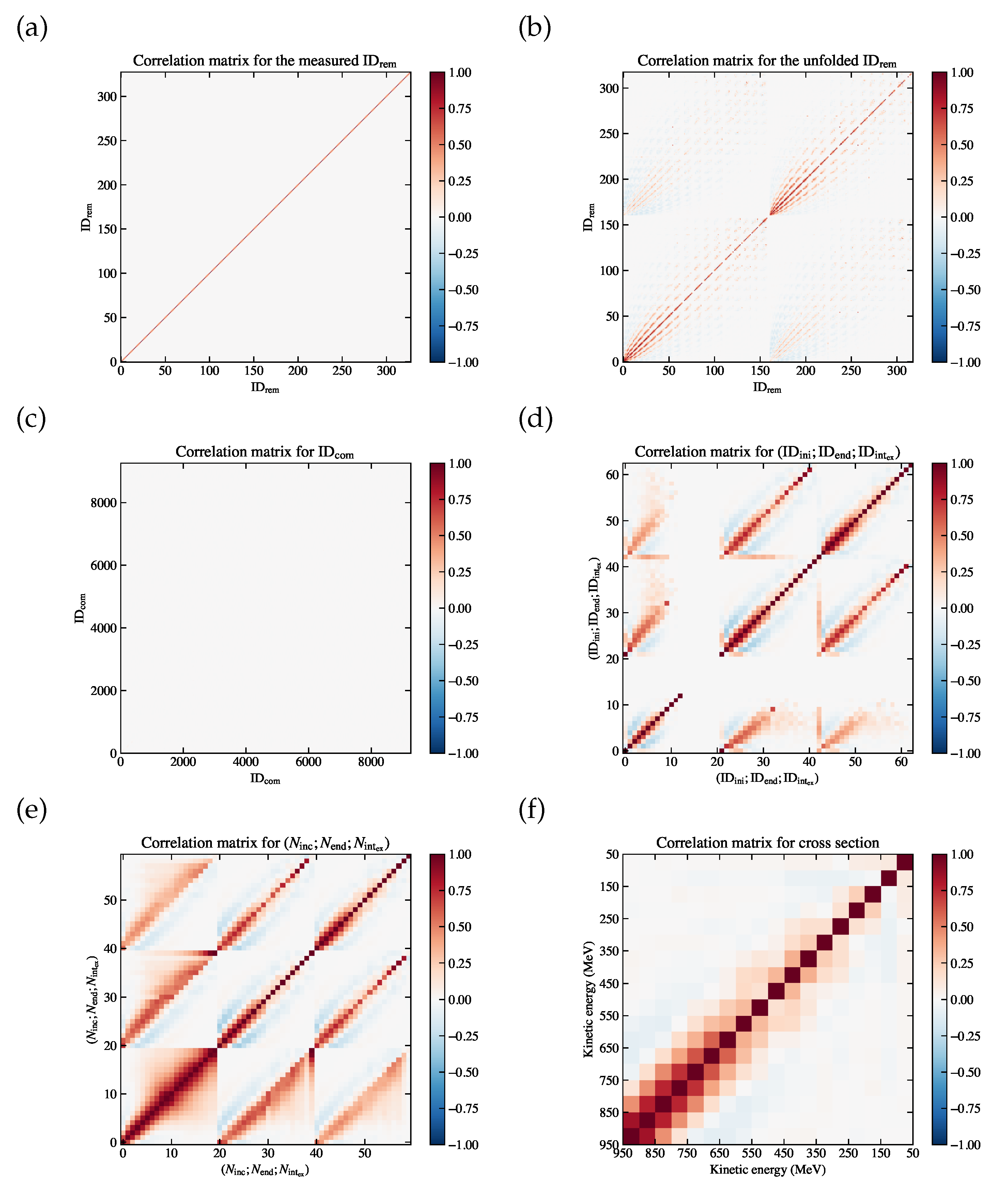
Figure 13.
The cross section measured using the unfolded histograms of the fake data sample. The reduced is approximately 1, which suggests good agreement between the sample and the input cross section.
Figure 13.
The cross section measured using the unfolded histograms of the fake data sample. The reduced is approximately 1, which suggests good agreement between the sample and the input cross section.
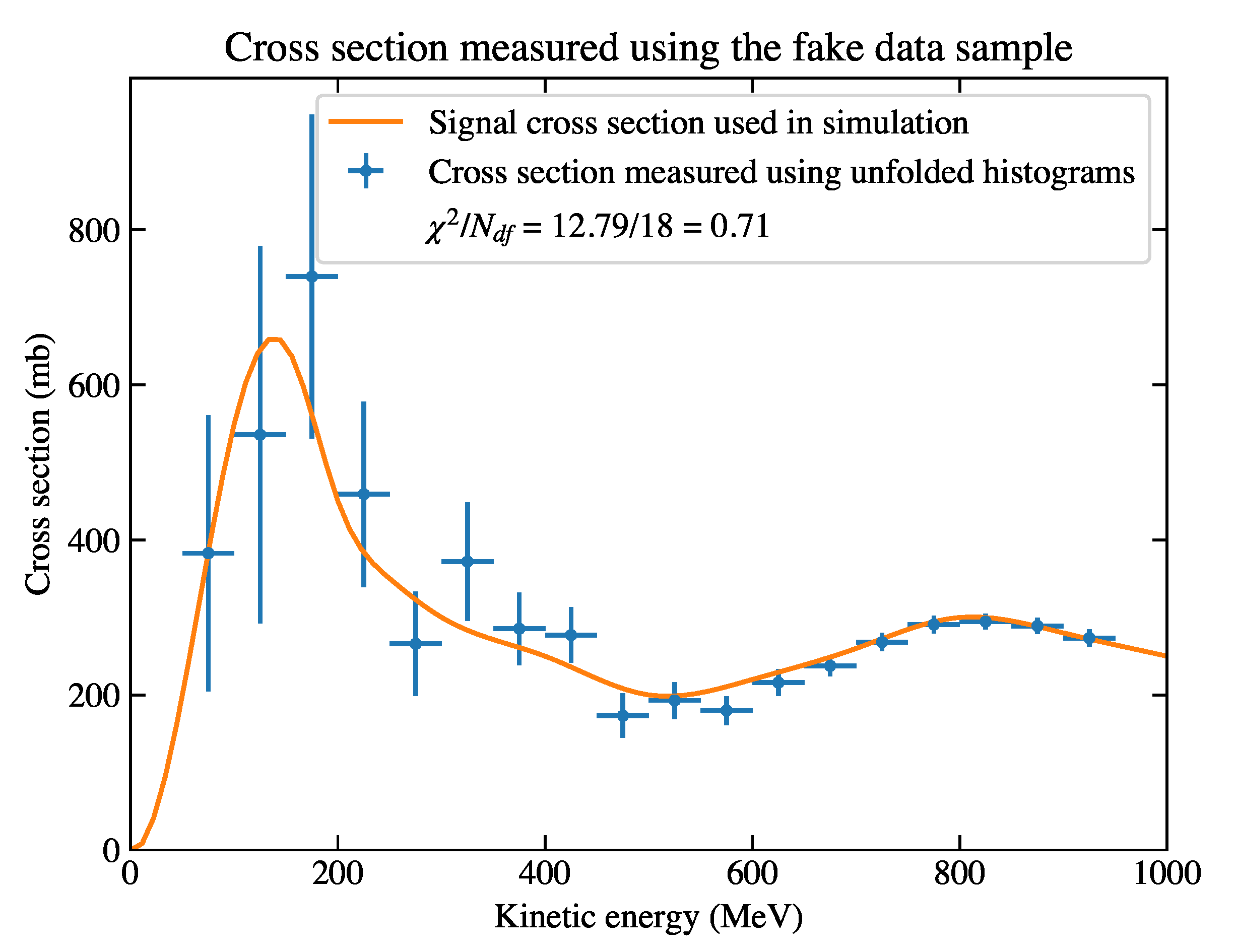
Figure 14.
Toy studies using the extracted true cross sections of 400 toy simulation samples. (a) The pull value test results. The horizontal axis is the energy slice index , where corresponds to the energy bin of MeV, and corresponds to the energy bin of MeV. The vertical axis is the pull value. The green lines are the pull values of each toy in each bin. The blue point and its error bars indicate and parameters of the Gaussian fit in each bin. The red lines sandwiching the blue point indicate the fit error of in each bin, which can be visually compared to the dashed orange line for its consistency with 0. The dark blue lines sandwiching the end points of the blue error bars indicate the fit error of in each bin, which can be visually compared to the dotted red line for its consistency with 1. (b) The histogram of against the simulation curve. Fitted distributions using both the maximum likelihood (MLH) fit and the least chi-square (LCS) fit are overlaid, with the result given in the legend.
Figure 14.
Toy studies using the extracted true cross sections of 400 toy simulation samples. (a) The pull value test results. The horizontal axis is the energy slice index , where corresponds to the energy bin of MeV, and corresponds to the energy bin of MeV. The vertical axis is the pull value. The green lines are the pull values of each toy in each bin. The blue point and its error bars indicate and parameters of the Gaussian fit in each bin. The red lines sandwiching the blue point indicate the fit error of in each bin, which can be visually compared to the dashed orange line for its consistency with 0. The dark blue lines sandwiching the end points of the blue error bars indicate the fit error of in each bin, which can be visually compared to the dotted red line for its consistency with 1. (b) The histogram of against the simulation curve. Fitted distributions using both the maximum likelihood (MLH) fit and the least chi-square (LCS) fit are overlaid, with the result given in the legend.
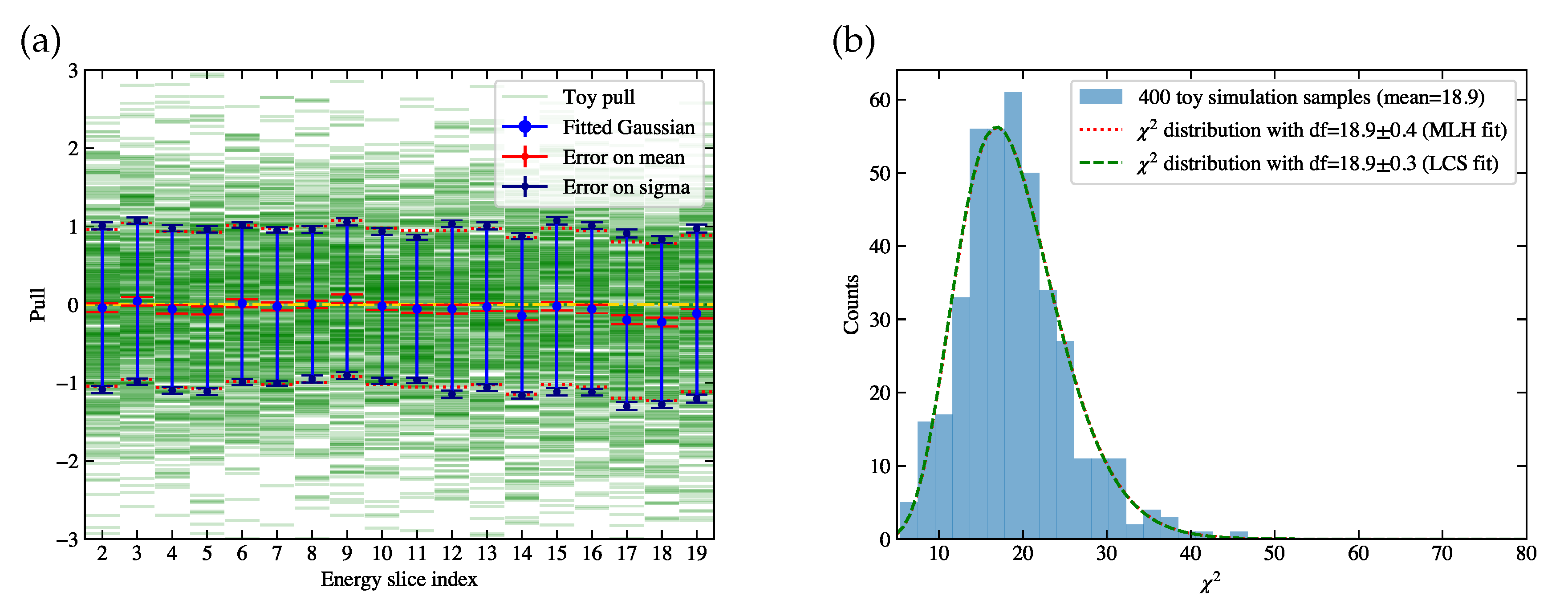
Figure 15.
Toy studies using the measured cross sections of 400 toy fake data samples. The detailed descriptions of subplots (a) and (b) are the same as described in Figure 14.
Figure 15.
Toy studies using the measured cross sections of 400 toy fake data samples. The detailed descriptions of subplots (a) and (b) are the same as described in Figure 14.
Disclaimer/Publisher’s Note: The statements, opinions and data contained in all publications are solely those of the individual author(s) and contributor(s) and not of MDPI and/or the editor(s). MDPI and/or the editor(s) disclaim responsibility for any injury to people or property resulting from any ideas, methods, instructions or products referred to in the content. |
© 2023 by the authors. Licensee MDPI, Basel, Switzerland. This article is an open access article distributed under the terms and conditions of the Creative Commons Attribution (CC BY) license (http://creativecommons.org/licenses/by/4.0/).
Copyright: This open access article is published under a Creative Commons CC BY 4.0 license, which permit the free download, distribution, and reuse, provided that the author and preprint are cited in any reuse.


