Network-Independent Synchronous Stability Boundary and Spontaneous Synchronization

1. Introduction

As the number of studies on collective behavior in complex systems has grown, synchronization in coupled systems has garnered extensive attention [1]. In addition, the study of generator synchronization has broader implications. In recent decades, synchronization in complex systems [1,2], e.g., synchronous discharge and the flashing of fireflies, is widely observed in nature and industry.

The current consensus is that synchronization is determined by both network structure and dynamics [2,3]. The network structure is the basis of the coupling matrix, and the dynamics require clear system parameters. However, this is difficult to achieve in practice [4,5]: complete observation of actual interactions proves challenging, while topological information may be incomplete [6]. Additionally, overly large networks make clear topology modeling quite difficult. These challenges can lead to incorrect network reconfiguration and link predictions. Even with complete topological information, real networks present additional challenges [7] including structural diversity, community structures, uncertain dynamics, and nonlinear parameters. There is also the massive amounts of data and the tedious calculations that come along with a huge network. These difficulties present substantial obstacles for the study of realistic network synchronization.

As the largest man-made network system, power systems are considered to be typical complex network systems. The generator oscillation equations are equivalent to the Kuramoto model [8] and the synchronization of generators is considered as an example of collective behavior of coupled oscillators in complex networks. Power grids are also considered as “small world networks” [9,10]. Therefore, the synchronization of power systems is also an important topic in the synchronization of complex networks [11]. This paper discusses the synchronization phenomenon of complex networks through power systems based on this understanding.

Synchronization is a prerequisite for the normal operation of a power grid and determines whether energy can be delivered to users. The difficulties of power system synchronization stability are a concrete manifestation of the above challenges in energy networks. Over the years, a number of approaches have been generated to analyze the laws governing the synchronous operation of generators [1,12,13]. These include the determination of synchronous stability boundaries for complex networks [1,14] and the use of spontaneous synchronization conditions [2].

The identification of the synchronous stability boundary is a key problem [15,16]. A stablity boundary is the union of critical points [17], and when the system state is outside the stability boundary, it is desynchronized [18]. As a cornerstone concept in grid synchronous stability intimately connected to numerous system issues [19], deriving analytical descriptions of the boundary has been a longstanding research objective [15,20,21]. On the other hand, the spontaneous synchronization of complex systems has been utilized to elucidate the synchronized operation of generators in interconnected grids [22]. Therefore, many studies on power system stability are based on the knowledge of synchronization conditions of complex networks [2,22,23]. While both paths have made great strides, however, current researches on synchronization are still limited by the abovementioned difficulties [22,24].

To overcome the abovementioned structural challenges, a network-independent synchronization analysis path is constructed in this paper. This paper derives and proves a power system synchronization stability boundary equation. The derivation here is heuristic and analogical. The equation describes the synchronous stability boundary of a power system in a unified manner and has elegant formal and physical interpretations. Mathematical proofs and experimental evidence ensure the rigor and validity of the boundary equation. These evidences demonstrate that this approach addresses the problems of the multiswing stability discrimination of multiple generators in a power system and partial synchronization. Subsequently, the results demonstrate that the synchronous stability boundary is independent of the network structure and parameters. It is also shown here that the synchronization stability of the power system is determined by the voltage, while the conclusion that both symmetry and asymmetry promote synchronization is discussed. In addition, the results provide clear evidence for the existence of a new type of spontaneous synchronization phenomenon in power systems. Comparison of the boundary with the occurrence of this phenomenon reveals that this novel spontaneous synchronization occurs only close to the boundary and may be manifested as a specific structure. This close connection suggests that, like the synchronization stability boundary, this spontaneous synchronization phenomenon is not directly related to the network. The approach in this paper identifies collective synchronization and non-synchronized units solely through the behavior of each generator in the system, specifically revealing synchronization mechanisms without prior knowledge of network structure, with extensively validation in power systems. This novel approach is developed to investigate the synchronization of grids in a unified way, taking into account potential scenarios of realistic network complexity, nonlinearity, or uncertainty. The results in this paper may inspire advances in other disciplines.

2. Methods

2.1. Power Grid Datasets

Here, we describe the sources of data for the two power-grid networks considered in this study, namely the 3-generator (3-gen) test system and the New England (10-gen) test system.

For each system, the data provide the generators’ dynamic parameters, the net injected real power at all generator nodes, the power demand at all nongenerator nodes, and the parameters of all power lines and transformers. These parameters are sufficient for standard power flow calculations and stability calculations [25].

WECC 3-generator test system (3-gen) [26]. This system represents the Western System Coordinating Council (WSCC), which is part of the region now called the Western Electricity Coordinating Council (WECC) in the North American power grid. There are 3 generators in the system.

New England test system (10-gen) [27]. The IEEE 39 bus system is the 10-machine New England Power System. The prototype of the IEEE 39-node system is a model of an actual power grid in New England. There are 10 generators in the system.

The significance of using two entirely distinct test systems is much greater than that of merely adding a few numerical results. More crucially, this serves to demonstrate the applicability of the assumption of this paper to a completely different network. These network models provide all the data sufficient for standard power flow calculations and stability calculations. The results of utilizing thn in Figure 2 and Figure 4, Figure S2, Figure S3, Figure S4 and Figure S5 and Table S1, and the results of utilizing the 3-generator test system are shown in Figure 3 and Figure S1.

2.2. Mathematical Model and Simulation Software

The swing equation can be used to analyze the synchronization of the generators. The expression of this equation is

$$\begin{array}{l}{\displaystyle \frac{d{\theta }_i}{dt}}={\omega }_i\\ I_i{\displaystyle \frac{d{\omega }_i}{dt}}=P_i-{\gamma }_i{\omega }_i+{\displaystyle \sum _{j=1}^N{K}_{ij}}\sin ({\theta }_j-{\theta }_i)\end{array}$$

(1)

where ${\gamma }_i$ is the damping of an oscillator, $I_i$ is the inertia constant and $K_{ij}$ is a coupling matrix governing the topology of the power grid network, and the strength of the interactions. ${\theta }_i$ is the voltage phase angle. This paper employs the power system models to analyze synchronization issues. Therefore, in order to conveniently obtain more accurate calculation results, each of the two models was simulated separately in this paper via the Power System Analysis Software Package [28] (PSASP), a simulation software. Standard power flow calculations and transient stability calculations were performed in the above network model using the software. Time series data of the generators’ response to network faults in the free state is collected. Map these data from generators $\left({u^{\prime }}_i(t),{{\delta }^{\prime }}_i(t)\right)$ to meta-generators $\left(u_i(t),{\delta }_i(t)\right)$ and visualize the results.

2.3. Experimental Steps

To validate the effectiveness of the boundary equations, the simulation experiment follows these general steps: Simulate line faults on the power grid model, calculate the system’s response to the faults, and test whether the boundary equation can effectively distinguish between stable and unstable responses.

Here, detailed steps are provided. First, we set up the networks of the test systems in the software package and input the data. This data is sourced from the aforementioned refs. 26 and 27, including power system component parameters, generator dynamic parameters, and so on. We first obtained steady-state data utilized the standard power flow calculation program. This serves as the foundation for dynamic calculations within the software package. The frequency base value is fixed at 50 Hz.

To observe the disturbed trajectory, we turned off the controls. Prior to performing dynamic calculations, we fixed the fault location (e.g., node 18 in the New England test system, as shown in Figure 2 and Figure 4) and specified the fault type and the fault clearing time $\Delta t$. In order to simulate the synchronization stability under large disturbances, all fault types discussed in this paper were set as a three-phase short circuit to ground. We calculated the rotation rate ${{\omega }^{\prime }}_i^{*}$ and port bus voltage ${u^{\prime }}_i(t)$ of the ith generator for various fault clearing times $\Delta t$. To test the effectiveness of the approach for the stability of multiple swings, the time window $T$ was set to 20 seconds. That is, using the start of the disturbance as a starting point, we calculated and recorded the generator data for the next 20 seconds. The fault location and type remain unchanged, a new fault clearing time $\Delta t+d(\Delta t)$ was set, and the above steps were repeated until the system loses synchronization stability (Figure 2(e) and Figure 3(d)). $d(\Delta t)$ denotes the step length.

The angle of rotation rate of the ith generator was subsequently calculated as ${{\delta }^{\prime }}_i(t)=2\arctan [{{\omega }^{\prime }}_i^{*}(t)]$. The extensive interconnections between generators make stability analysis very challenging (see Figure S2). Figure S2 demonstrates the necessity of Equation (2). This challenge arises from the complexity of the network. In order to analyze the phenomenon of partial synchronization, the concept of a meta-generator is introduced here. At moment t, the instantaneous values of the n generator system $\left({u^{\prime }}_i(t),{{\delta }^{\prime }}_i(t)\right),i=1,2,\mathrm{...},n$ are arranged in descending order by ${\delta }_{\omega }$, relabeled, and then reconstituted as the n meta-generator system $\left(u_i(t),{\delta }_i(t)\right),i=1,2,\mathrm{...},n$.

In other words, when the condition ${{\delta }^{\prime }}_{i+1}(t)>{{\delta }^{\prime }}_i(t)$ holds, we relabel the serial number of the generator at that moment:

$$\begin{array}{l}(u_{i+1}(t),{\delta }_{i+1}(t))=({u^{\prime }}_i(t),{{\delta }^{\prime }}_i(t)),\\ \left(u_i(t),{\delta }_i(t)\right)=\left({u^{\prime }}_{i+1}(t),{{\delta }^{\prime }}_{i+1}(t)\right).\end{array}$$

(2)

A meta-generator is created by reordering and labeling generators. This is a technical treatment only, and this transformation has been shown not to change the stability of the system [refer to “Proof that Equation (2) does not alter the stability criterion of the system”]. In this way, we obtain the meta-generator data $\left(u_i(t),{\delta }_i(t)\right),i=1,2,\mathrm{...},n$. Before and after the transformation, the numbers of generators and meta-generators are equal. Except for Figures S2 and S3, all results and discussions in this paper are based on the meta-generator.

2.4. Data Calculation

The polar coordinates of the ith meta-generator are denoted by $（u_i,{\delta }_i)$ [see Figure 1]. The 3D coordinate point formed by the Kth and Lth meta-generators is denoted by $（u_K,u_L,{\delta }_{K,L})$ [see Figure 2]. These points are calculated as follows:

The means of $\left(u_i(t),{\delta }_i(t)\right),i=1,2,\mathrm{...},n$ over $\left[0,T\right]$ were

$$\begin{array}{l}{u}_i={\displaystyle \frac{1}{T}}{\displaystyle {\int }_0^T{u}_i(\tau )d\tau },\\ {\delta }_i={\displaystyle \frac{1}{T}}{\displaystyle {\int }_0^T{\delta }_i(\tau )d\tau }\end{array}$$

(3)

And

$$\begin{array}{l}{\delta }_{K,L}={\displaystyle \frac{1}{T}}{\displaystyle {\int }_0^T{\delta }_{K,L}(\tau )d\tau }={\displaystyle \frac{1}{T}}{\displaystyle {\int }_0^T\left|{{\delta }^{\prime }}_K(\tau )-{{\delta }^{\prime }}_L(\tau )\right|d\tau }\\ ={\displaystyle \frac{1}{T}}{\displaystyle {\int }_0^T{\delta }_K(\tau )-{\delta }_L(\tau )d\tau }={\delta }_K-{\delta }_L.\end{array}$$

(4)

The results are shown in Figures 2(b), 4(b), S1(a), etc.

The means of $\left(u_i(t),{\delta }_i(t)\right),i=1,2,\mathrm{...},n$ over $[T,T+dT]$ were

$$\begin{array}{l}{u}_i(dT)={\displaystyle \frac{1}{dT}}{\displaystyle {\int }_T^{T+dT}{u}_i(\tau )}d\tau ,\\ {\delta }_{K,L}(dT)={\delta }_K(dT)-{\delta }_L(dT)={\displaystyle \frac{1}{dT}}{\displaystyle {\int }_T^{T+dT}\left[{\delta }_K(\tau )-{\delta }_L(\tau )\right]}d\tau ,\end{array}$$

(5)

where $dT$ is the time interval. The results are shown in Figures 2(c) and 3(b).

The standard deviation of ${\delta }_i$ is calculated as follows:

$$\begin{array}{l}\sigma \left({\delta }_i\right)=\sqrt{{\displaystyle \frac{{\displaystyle \sum _{i=1}^n{({\delta }_i-E\left({\delta }_i\right))}^2}}{n}}},\\ E\left({\delta }_i\right)={\displaystyle \frac{{\displaystyle \sum _{i=1}^n{\delta }_i}}{n}}.\end{array}$$

(6)

where $E\left({\delta }_i\right)$ is the expectation of ${\delta }_i$. The results are shown in Figures 4(a), S1(a) and S4.

2.5. Derivation of the Boundary Equation and Visualization

Synchronization emerges when the suppression dominates dissimilarity. Suppression includes the effects of coupling and dissipation, etc. Currently, the coupling is usually quantified by coupling using graph theory, and the dissimilarity is quantified by the frequencies ${\omega }_i$.²

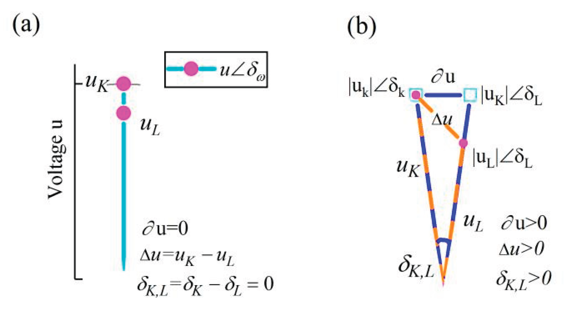
Figure 1. and $\partial u$ in the polar coordinate. Figure 1 is an analogy of a phasor diagram, which is one of the tools for power system analysis. The amplitude in polar coordinates is voltage $u_i$, and the angle is calculated from frequency ${\omega }_i$. (Figure 1 is a schematic diagram for illustrative purposes and analogy, not based on actual data.) $\Delta u$ is defined as “the suppression potential difference” between the Kth and Lth generators. $\partial u$ is constructed to describe “the dissimilar potential difference” between the Kth and Lth meta-generators. $\left|\Delta u\right|$ and $\left|\partial u\right|$ are calculated using Equation (9). (a). Phasor diagram during synchronous operation of meta-generators. The magenta dot indicates the ith meta-generator’s coordinates $\left|u_i\right|\angle {\delta }_i$ in the phasor diagram. The length of the solid cyan line represents the voltage of the ith meta-generator $u_i$. The angle of the solid line is defined as the angle of rotation rate of the ith meta-generator ${\delta }_i=2\arctan ({\omega }_i^{*})=2\arctan ({\displaystyle \frac{{\omega }_i}{{\omega }_0}})$, where ${\omega }_0$ represents the power system base frequency and ${\omega }_i$ is actual value. Specifically, for the power system, when the meta-generator operates synchronously, ${\omega }_1^{*}={\omega }_2^{*}=\mathrm{...}={\omega }_n^{*}=1$ and ${\delta }_i={\displaystyle \frac{\pi }{2}},i=1,2,\mathrm{...},n$. The angular difference ${\delta }_{K,L}$ is 0 and $\left|\Delta u\right|=\left|{\overrightarrow{u}}_K-{\overrightarrow{u}}_L\right|\ge \left|\partial u\right|=0$. (b). Polar coordinate diagram of the meta-generator in asynchronous operation. The length of the orange dotted line between the magenta square dots represents $\Delta u$and The length of the solid blue line between the cyan dots represents $\partial u$. When the meta-generator frequencies differ, ${\omega }_K^{*}\ne {\omega }_L^{*}$ then ${\delta }_{K,L}>0$. There are $\left|\Delta u\right|>0$ and $\left|\partial u\right|>0$.

Figure 1. and $\partial u$ in the polar coordinate. Figure 1 is an analogy of a phasor diagram, which is one of the tools for power system analysis. The amplitude in polar coordinates is voltage $u_i$, and the angle is calculated from frequency ${\omega }_i$. (Figure 1 is a schematic diagram for illustrative purposes and analogy, not based on actual data.) $\Delta u$ is defined as “the suppression potential difference” between the Kth and Lth generators. $\partial u$ is constructed to describe “the dissimilar potential difference” between the Kth and Lth meta-generators. $\left|\Delta u\right|$ and $\left|\partial u\right|$ are calculated using Equation (9). (a). Phasor diagram during synchronous operation of meta-generators. The magenta dot indicates the ith meta-generator’s coordinates $\left|u_i\right|\angle {\delta }_i$ in the phasor diagram. The length of the solid cyan line represents the voltage of the ith meta-generator $u_i$. The angle of the solid line is defined as the angle of rotation rate of the ith meta-generator ${\delta }_i=2\arctan ({\omega }_i^{*})=2\arctan ({\displaystyle \frac{{\omega }_i}{{\omega }_0}})$, where ${\omega }_0$ represents the power system base frequency and ${\omega }_i$ is actual value. Specifically, for the power system, when the meta-generator operates synchronously, ${\omega }_1^{*}={\omega }_2^{*}=\mathrm{...}={\omega }_n^{*}=1$ and ${\delta }_i={\displaystyle \frac{\pi }{2}},i=1,2,\mathrm{...},n$. The angular difference ${\delta }_{K,L}$ is 0 and $\left|\Delta u\right|=\left|{\overrightarrow{u}}_K-{\overrightarrow{u}}_L\right|\ge \left|\partial u\right|=0$. (b). Polar coordinate diagram of the meta-generator in asynchronous operation. The length of the orange dotted line between the magenta square dots represents $\Delta u$and The length of the solid blue line between the cyan dots represents $\partial u$. When the meta-generator frequencies differ, ${\omega }_K^{*}\ne {\omega }_L^{*}$ then ${\delta }_{K,L}>0$. There are $\left|\Delta u\right|>0$ and $\left|\partial u\right|>0$.

Here, the suppression strength between the nodes is quantified by $P_{\Delta u}$ and the dissimilarity between the nodes is quantified by $P_{\partial u}$. $P_{\Delta u}$ and $P_{\partial u}$ have the same dimension and can be directly compared in size. In power systems, there are

$$P_{\Delta u}={\displaystyle \frac{{\left|{\overrightarrow{u}}_K-{\overrightarrow{u}}_L\right|}^2}{\left|Z_{K,L}\right|}}={\displaystyle \frac{{\left|\Delta u\right|}^2}{\left|Z_{K,L}\right|}}$$

(7)

and

$$P_{\partial u}={\displaystyle \frac{{\left|{\overrightarrow{u}}_K-\frac{\left|{\overrightarrow{u}}_K\right|}{\left|{\overrightarrow{u}}_L\right|}{\overrightarrow{u}}_L\right|}^2}{\left|Z_{K,L}\right|}}={\displaystyle \frac{{\left|\partial u\right|}^2}{\left|Z_{K,L}\right|}}$$

(8)

[see Figure 1(b)]. The expressions for $P_{\Delta u}$ and $P_{\partial u}$ are analogous to those of $P_{K,L}={\displaystyle \frac{{\left|{\stackrel{\rightharpoonup }{U}}_K-{\stackrel{\rightharpoonup }{U}}_L\right|}^2}{\left|Z_{K,L}\right|}}$, which can represent the rate of energy dissipation between the nodes in a power system. This dissipation is the kind of suppression that includes energy lost in resistance and stored in inductance or capacitance. $Z_{K,L}$ is the impedance between the Kth and Lth meta-generators. The meta-generator is “the map of the generator” and defined by Equation (2). Both the suppression strength and dissimilarity vary with individual behavior. The difference between ${\stackrel{\rightharpoonup }{u}}_i$ and $\stackrel{\rightharpoonup }{U}$ is that the angle ${\delta }_i$ of ${\stackrel{\rightharpoonup }{u}}_i$ is defined by the frequencies ${\omega }_i$ while the angle of $\stackrel{\rightharpoonup }{U}$ is the phase angle. The voltage phasor diagram was one of the inspirations.

For real power systems, when all oscillators are complete synchronized (i.e., ${\omega }_1={\omega }_2=\mathrm{...}={\omega }_n$), $P_{\Delta u}$ is usually greater than 0 because the meta-generator voltages $u_K$ and $u_L$ are often unequal and $P_{\partial u}=0$ because there is no dissimilarity in the frequencies ${\omega }_i$ (${\delta }_{K,L}=0,\Delta u>0,\partial u=0$) [see Figure 1(a)]. Following a disturbance in the power system, the meta-generators’ rotational speeds are dissimilar, $P_{\partial u}>0$ (${\delta }_{K,L}>0,\Delta u>0,\partial u>0$) [see Figure 1(b)]. Considering the synchronization occurrence condition mentioned earlier, the boundary equation is expressed as $P_{\Delta u}=P_{\partial u}$ in the grid. When $\left|P_{\partial u}\right|\le \left|P_{\Delta u}\right|$, the system is synchronous and stable. Conversely, when $\left|P_{\partial u}\right|>\left|P_{\Delta u}\right|$, the system is out of synchronization and unstable.

I emphasize that $\left|P_{\partial u}\right|/\left|P_{\Delta u}\right|=1$, not $P_{\Delta u}$ and $P_{\partial u}$, is independent of the network topology. It is clear from the form of $P_{\Delta u}$ and $P_{\partial u}$ that they are related to the network, as information about the network is contained in $Z_{K,L}$. For any two meta-generators K and L, $Z_{K,L}$ is the same in the expressions for $P_{\Delta u}$ and $P_{\partial u}$. Therefore, $\left|P_{\partial u}\right|/\left|P_{\Delta u}\right|=1$ eliminates $Z_{K,L}$. It is observed that $\left|P_{\partial u}\right|/\left|P_{\Delta u}\right|=1\iff \left|\partial u\right|/\left|\Delta u\right|=1$. The set of points for which $\left|\partial u\right|=\left|\Delta u\right|$ is the synchronous stability boundary.

As shown in Figure 1(b),

$$\begin{array}{l}\left|\Delta u\right|=\left|{\overrightarrow{u}}_K-{\overrightarrow{u}}_L\right|=\sqrt{u_K^2+u_L^2-2u_K{u}_L\cos {\delta }_{K,L}},\\ \left|\partial u\right|=\left|{\overrightarrow{u}}_K-{\displaystyle \frac{\left|{\overrightarrow{u}}_K\right|}{\left|{\overrightarrow{u}}_L\right|}}{\overrightarrow{u}}_L\right|=\sqrt{2u_K^2(1-\cos {\delta }_{K,L})}.\end{array}$$

(9)

The symbols “∆” and “∂” are for distinction only and have no mathematical significance. Thus, the boundary equation is obtained via derivation from ${\left|{\overrightarrow{u}}_K\right|}^2+{\left|{\overrightarrow{u}}_L\right|}^2-2\left|{\overrightarrow{u}}_K\right|\left|{\overrightarrow{u}}_L\right|\cos {\delta }_{K,L}=2{\left|{\overrightarrow{u}}_K\right|}^2(1-\cos {\delta }_{K,L})$. The only variables in the boundary equation are $u_K,u_L$ and ${\delta }_{K,L}$.

$f\left(u_K,u_L,{\delta }_{K,L}\right)=\left|\partial u\right|/\left|\Delta u\right|=1$ is the stability boundary equation. When $\left|\partial u\right|/\left|\Delta u\right|<1$, the system is stable. When $\left|\partial u\right|/\left|\Delta u\right|>1$, the system is unstable. Geometrically, $f\left(u_K,u_L,{\delta }_{K,L}\right)=1$ describes exactly curved surfaces that, together with $(0,u_L,{\delta }_{K,L})$, $(u_K,0,{\delta }_{K,L})$ and $(u_K,u_L,0)$ enclose a stable domain.

In summary, the boundary equation

$$\left|u_K\right|=\left|u_L\right|\cup {\displaystyle \frac{\left|u_L\right|}{\left|u_K\right|}}=2\cos {\delta }_{K,L}-1$$

(10)

can be found, where $\left|u_K\right|\ge \left|u_L\right|\ge 0,\left|{\delta }_{K,L}\right|\ge 0$.

The derivations and parameter selections and transformations here, such as $P_{\Delta u}$, $P_{\partial u}$, and ${\delta }_i=2\arctan ({\omega }_i^{*})$, are heuristic and analogical. They do not stem from dynamical models or prior literature, thus requiring experimental validation and mathematical proof. Experimental validation is provided in Figures 2, 3, S2, S3(b) and S5, and Table S1, among others. Mathematical proof is detailed in “Proof of the Boundary Equation.” The coordinate system $u_K-u_L-{\delta }_{K,L}$ is established, and the boundary is visualized (Figure 2(a)).

The boundary equation without ${\omega }_0$As mentioned in the derivation above: ${\delta }_i=2\arctan ({\omega }_i^{*})=2\arctan ({\displaystyle \frac{{\omega }_i}{{\omega }_0}})$, where ${\omega }_0$ represents the power system base frequency and ${\omega }_i$ is actual value. ${\omega }_0$ is constrained to positive real numbers. For a power system, the base frequency generally coincides with the system’s rated frequency (50 Hz or 60 Hz in most power grids globally). As previously stated in this paper, ${\omega }_0=50Hz$. ${\omega }_0$ is widely used in power system analysis. However, to some extent, the selection of ${\omega }_0$ remains “anthropic selective”. Also, ${\omega }_0$ may be unknown before synchronization emerges. Can ${\omega }_0$ be eliminated from the boundary equation? i.e., is there a synchronization stability boundary independent of ${\omega }_i$ for power systems?

When ${\delta }_i=2\arctan {\displaystyle \frac{{\omega }_i}{{\omega }_0}}$ is substituted into Equation (10),

$${\displaystyle \frac{1}{2}}({\displaystyle \frac{\left|u_L\right|}{\left|u_K\right|}}+1)=\cos [2(\arctan {\displaystyle \frac{{\omega }_K}{{\omega }_0}}-\arctan {\displaystyle \frac{{\omega }_L}{{\omega }_0}})]$$

(11)

Considering $\cos 2\alpha ={\displaystyle \frac{1-{\tan }^2\alpha }{1+{\tan }^2\alpha }}$ and $\tan (\alpha -\beta )={\displaystyle \frac{\tan \alpha -\tan \beta }{1+\tan \alpha \tan \beta }}$,

$${\displaystyle \frac{1}{2}}({\displaystyle \frac{\left|u_L\right|}{\left|u_K\right|}}+1)={\displaystyle \frac{{\left({{\omega }_0}^2+{\omega }_K{\omega }_L\right)}^2-{{\omega }_0}^2{\left({\omega }_K-{\omega }_L\right)}^2}{{\left({{\omega }_0}^2+{\omega }_K{\omega }_L\right)}^2+{{\omega }_0}^2{\left({\omega }_K-{\omega }_L\right)}^2}}$$

(12)

By setting $A^{\prime }=\sqrt{{\displaystyle \frac{\left|u_K\right|-\left|u_L\right|}{3\left|u_K\right|+\left|u_L\right|}}},B^{\prime }={\omega }_L-{\omega }_K,C^{\prime }={\omega }_L{\omega }_K\sqrt{{\displaystyle \frac{\left|u_K\right|-\left|u_L\right|}{3\left|u_K\right|+\left|u_L\right|}}}$, Equation (12) becomes $A^{\prime }{{\omega }_0}^2+B^{\prime }{\omega }_0+C^{\prime }=0$. Therefore,

$${\omega }_{01,2}={\displaystyle \frac{{\omega }_K-{\omega }_L\pm \sqrt{{\left({\omega }_K-{\omega }_L\right)}^2-4\frac{\left|u_K\right|-\left|u_L\right|}{3\left|u_K\right|+\left|u_L\right|}{\omega }_L{\omega }_K}}{2\sqrt{\frac{\left|u_K\right|-\left|u_L\right|}{3\left|u_K\right|+\left|u_L\right|}}}}$$

(13)

For real-world systems, both ${\omega }_{01}$ and ${\omega }_{02}$ must be real numbers. There is a constraint that ${\left({\omega }_K-{\omega }_L\right)}^2-4{\displaystyle \frac{\left|u_K\right|-\left|u_L\right|}{3\left|u_K\right|+\left|u_L\right|}}{\omega }_L{\omega }_K\ge 0$. Therefore, the power system is synchronously stable when

$$1-{\displaystyle \frac{4{\left({\omega }_K-{\omega }_L\right)}^2}{{\left({\omega }_K+{\omega }_L\right)}^2}}\le {\displaystyle \frac{\left|u_L\right|}{\left|u_K\right|}}\le 1$$

(14)

$$1-{\displaystyle \frac{4{\left({\omega }_K-{\omega }_L\right)}^2}{{\left({\omega }_K+{\omega }_L\right)}^2}}={\displaystyle \frac{\left|u_L\right|}{\left|u_K\right|}}$$

(15)

is the stability boundary without ${\omega }_0$. When $u_K=u_L$, Any value chosen for ${\omega }_K-{\omega }_L\ge 0$ satisfies Equation (14). $u_K=u_L$ is exactly the left side of Equation (10). When $u_K\ne u_L$, Equation (15) is equivalent to the right side of Equation (10) [see Proof of Equivalence Between Equations (10) and (15)]. This boundary equation is still determined by the behavior of individuals in the system and is independent of the network.

Comparing Equation (10) and Equation (15), Equation (15) has a broader range of applicability since Equation (10) requires prior knowledge of the value of ${\omega }_0$. However, for convenience, this paper still uses Equation (10) for visualization, as shown in Figure 2(a).

3. Results and Discussion

3.1. Stability Boundary

Synchronization occurs when the suppression dominates the dissimilarity. In power systems, the suppression is denoted as and the dissimilarity is denoted as . That is, when , the system is synchronous and stable, otherwise it is out of synchronization. Therefore, represents the synchronous stability boundary.

To facilitate the discussion of the validity of the synchronous boundary equation of power system, Equation (10) is restated here:

$$\left(\left|u_K\right|=\left|u_L\right|\right)\cup \left(\left|u_L\right|/\left|u_K\right|=2\cos {\delta }_{K,L}-1\right)$$

where $\left|u_K\right|>\left|u_L\right|\ge 0,\left|{\delta }_{K,L}\right|\ge 0$. (see Derivation of the boundary equation and Proof of the boundary equation)

Here, ${\delta }_K=2\arctan ({\omega }_K)$ is defined as the angle of rotation rate of the Kth meta-generator. It is important to note that ${\delta }_K$ is not a phase and that $L=K+1$. Equation (10) actually defines the synchronous stability boundary for two meta-generators, hence $L=K+1$. For multi-generators systems, since all boundary equations share identical forms, the visualized graphs completely coincide, as shown in Figure 2(a). The angle difference of rotation rate between the Kth and Lth meta-generators is ${\delta }_{K,L}=\left|{\delta }_K-{\delta }_L\right|\ge 0$. According to the definition of synchronization, ${\delta }_1=\dots ={\delta }_K={\delta }_L=\dots ={\delta }_n$. $u_K,u_L$ denote the voltages of the Kth and Lth meta-generators, respectively. The meta-generators are “the map of the generators” (refer to Equation (2)). The voltage has been previously overlooked for simplicity [22,29] but is crucial for the synchronization stability of the grid. ${\omega }_i$ is the frequency of the ith meta-generator, which is a normalization quantity commonly used in power system studies.

Figure 2. Validity of stability boundary (Meta-generators in the 10-gen).

Figure 2. Validity of stability boundary (Meta-generators in the 10-gen).

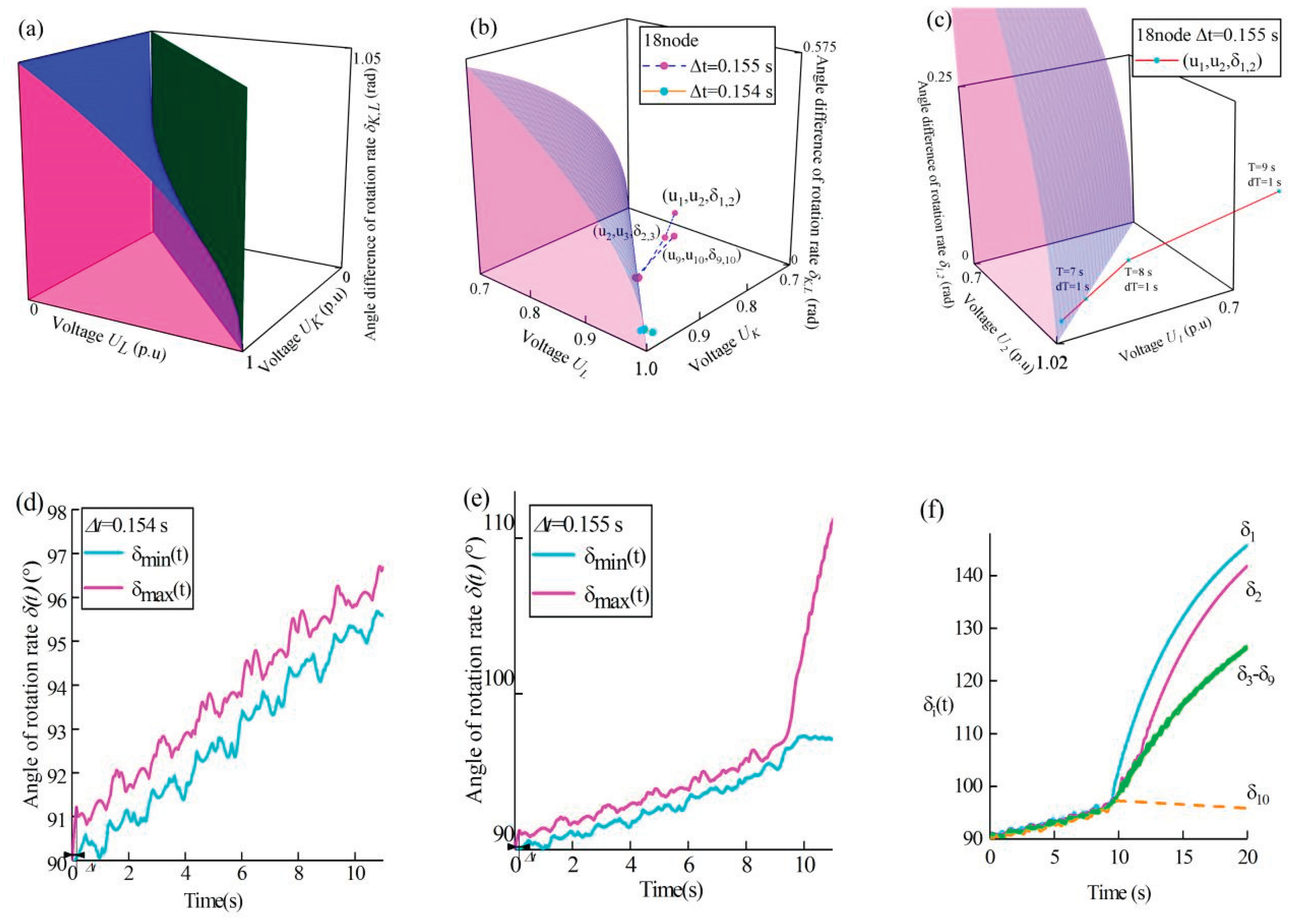
A New England test system was used. A three-phase short-circuit ground fault occurred at node 18. The data in Figure 2 is derived from numerical simulations experiments. $\Delta t$ is the fault clearing time. $d(\Delta t)=0.001 s$ denotes the step length commonly used in power system studies.

(a). Visualization of the stability boundary. The stability boundary in Equation (10) (blue surface and dark green plane) and the pink planes $0-u_L-{\delta }_{K,L}$, $u_K-0-{\delta }_{K,L}$ and $u_K-u_L-0$ collectively define the boundaries and enclose the stability domain.

(b). Synchronization stability assessment and partial synchronization. $(u_K,u_L,{\delta }_{K,L})$ is defined as the 3D coordinate point formed by the Kth and Lth meta-generators, and it is computed from $u_K, {\delta }_K, u_L$ and ${\delta }_L$. $(u_K,u_L,{\delta }_{K,L})$ are calculated using Equations (3) and (4). The cyan and magenta points represent the position of $(u_K,u_L,{\delta }_{K,L})$ when $\Delta t=0.154s$ and $\Delta t=0.155 s$, respectively.

(c). The process of meta-generator desynchronization and the stability of multiple swings for multiple generators. The disturbed trajectory of $\left(u_1,u_2,{\delta }_{1,2}\right)$ is selected ($\Delta t=0.155 s$). The calculation range is $6s\le T\le 9s$. Each cyan point represents the mean position of $\left(u_1,u_2,{\delta }_{1,2}\right)$ for a period of 1 second. The time T and the time interval $dT=1s$ are defined in Equation (5).

(d) and (e). Experimental verification of synchronous stability and the stability of multiple swings for multiple generators($\Delta t=0.154s$ and $\Delta t=0.155 s$). The horizontal axis represents the time. The vertical axis represents the value of ${\delta }_i(t)$. The maximum value of ${\delta }_i(t)$ is represented by the magenta curve, and the minimum value is represented by the cyan curve. ${\delta }_{\min }(t)\le {\delta }_i(t)\le {\delta }_{\max }(t)$. At 11 second, ${\delta }_{\max }(t)-{\delta }_{\min }(t)\approx 1°$ in (d), and ${\delta }_{\max }(t)-{\delta }_{\min }(t)\approx 14°$ in (e). As illustrated in panel (d), the ${\delta }_i(t)$ values of all meta-generators are close to each other and have approximately the same rate of change. panel (e) shows that in the time interval $(9s,10s)$, ${\delta }_{\max }(t)-{\delta }_{\min }(t)$ increases sharply, indicating generator desynchronization.

(f). Experimental verification of partial synchronization. $\Delta t=0.155 s$. The horizontal axis represents the time. The vertical axis represents the value of ${\delta }_i(t)$. After approximately 9 seconds, meta-generator 1 disengages from the cluster (cyan line). Subsequently, meta-generators 10 (magenta line) and 2 (orange dashed line) are separated. Meta-generators 3~9 form a synchronized cluster (green lines). ${\delta }_i(t)$ are calculated using simulation software and Equation (2).

Three pieces of evidence demonstrate that Equation (10) effectively describes the synchronization stability boundary: 1) the boundary effectively distinguishes between stable and unstable states of the power system [see Figures 2(b) and 3(a)], 2) the stability of multiple swings [see Figures 2(c) and 3(b)], and 3) the partial synchronization phenomenon [see Figures 2(f) and 3(e)].

Figure 2(b) illustrates that the synchronization stability boundary effectively differentiates between synchronized and desynchronized states. A system comprising n meta-generators ‌possesses n-1 3D coordinate points. The behavior of the cyan and magenta dots is significantly different, despite the slight difference in $\Delta t$ (Figure 2(b)). When $\Delta t=0.154 s$, all of the cyan dots are clustered at the boundary. When $\Delta t=0.155 s$, the three magenta dots, i.e., $(u_1,u_2,{\delta }_{1,2})$, $(u_2,u_3,{\delta }_{2,3})$, and $(u_9,u_{10},{\delta }_{9,10})$, are outside the boundary and away from the rest of points. As mentioned above, when $P_{\Delta u}<P_{\partial u}$, $(u_K,u_L,{\delta }_{K,L})$ is outside the boundary and the power system is out of synchronization. Consequently, it is concluded that the power system is stable at $\Delta t=0.154s$ and out of synchronization at $\Delta t=0.155s$. The results in Figures 2(d) and (e) are in good agreement with this conclusion. Additional analogous results can be found in Figure S5.

Furthermore, utilizing Figure 2(b) facilitates easily identify different synchronization patterns as it provides specific information about synchronized and desynchronized individual meta-generators or groups of meta-generators. The New England test system comprises 10 meta-generators, which is equivalent to 9 dots in Figure 2. As shown in Figure 2(b), $(u_1,u_2,{\delta }_{1,2})$,$(u_2,u_3,{\delta }_{2,3})$ and $(u_9,u_{10},{\delta }_{9,10})$ are outside the boundary while the rest of the points are clustered near the boundary. This signify that the meta-generators are divided into 4 synchronization groups. Specifically, $(u_1,u_2,{\delta }_{1,2})$ outside the boundary means that the meta-generators 1 and 2 are not synchronized. There are analogous conclusions for $(u_2,u_3,{\delta }_{2,3})$ and $(u_9,u_{10},{\delta }_{9,10})$. That is, the meta-generators numbered 1, 2 and 10 are out of synchronization while the other meta-generators remain synchronized. This indicates that the meta-generators in each group are also clearly shown in Figure 2(b). The result for the meta-generator synchronization group shown in Figure 2(f) is in good agreement with those presented in Figure 2(b). This is the phenomenon of cluster synchronization [30,31]. Current research suggests that cluster synchronization occurs for a variety of reasons [32,33]. These results suggest that these causes can be described as the loss of synchronization stability between the oscillators corresponding to certain coordinate points and splitting into different synchronized clusters when these points lie outside the boundary. This interpretation will deepen our understanding of the complex phenomenon of partial synchronization. [More evidence can be found in Table S1 in Supplemental Material.]

Figure 2(c) shows the transition of the power system from stabilization to instability. As shown in Figure 2(c), $(u_1,u_2,{\delta }_{1,2})$ crosses the boundary outwardly during the time interval $(8s,9s)$. Subsequently, ${\delta }_{1,2}$ increases dramatically during the time interval $(9s,10s)$. These results are in good agreement with the simulation result presented in Figure 2(e). This also suggests that the assumption of ignoring voltage [8] variations may fail even for short-term simulations(of the order of one second or less). The simulation result demonstrates that the system loses synchronization during the aforementioned time interval. Therefore, the time at which the 3D coordinate point crosses the boundary is the onset of synchronization loss. These results pertain to the stability of multiple swings for multiple generators, an important issue that has not been resolved to date [34,35]. The above results demonstrate the synchronization stability boundary expressed by Eq.(10) can discriminate the stability of multiple swings for multiple generators in real time. Comparison of the results in Figures 2(b) and (c) reveals that the synchronous stability boundary is applicable to different time scales in power systems (long-term and short-term dynamics). More importantly, these results show that the synchronization stability boundary is the same in various cases (multi-machine, multi-swing scenarios, cluster synchronization situations, and different time scales). To power systems, this helps analyze the synchronous stability in a unified way.

The numerical experimental results in Figures 2(d), (e) and (f) are time-series data independently calculated by the simulation software. The results in Figures 2(b) and (c) are in good agreement with these experimental data. The above results provide solid evidences for the correctness and validity of the boundary equation from various perspectives.

As shown in Figure 2(a), geometrically, Equation (10) represents two surfaces in a coordinate system $u_K-u_L-{\delta }_{K,L}$. The left-hand side of Equation (10) corresponds to a plane (dark green) perpendicular to the plane $u_K-u_L$, and the right-hand side corresponds to a curve surface (blue). These two surfaces are fixed, i.e., they are independent of network topology and parameters. Therefore, Equation (10) is independent of the network topology, system parameters, perturbations and number of subsystems. This finding, which contradicts previous reports [2,15,20], indicates that the stability boundary of power system is independent of these factors. It is emphasized that ${\displaystyle \frac{\left|P_{\partial u}\right|}{\left|P_{\Delta u}\right|}}=1$, not and , is independent of the network topology. The impact of the network is nullified through division (refer to “Derivation of the boundary equation”).

Figure 3. Network-independent synchronous stability boundary. (Meta-generators in the 3-gen).

Figure 3. Network-independent synchronous stability boundary. (Meta-generators in the 3-gen).

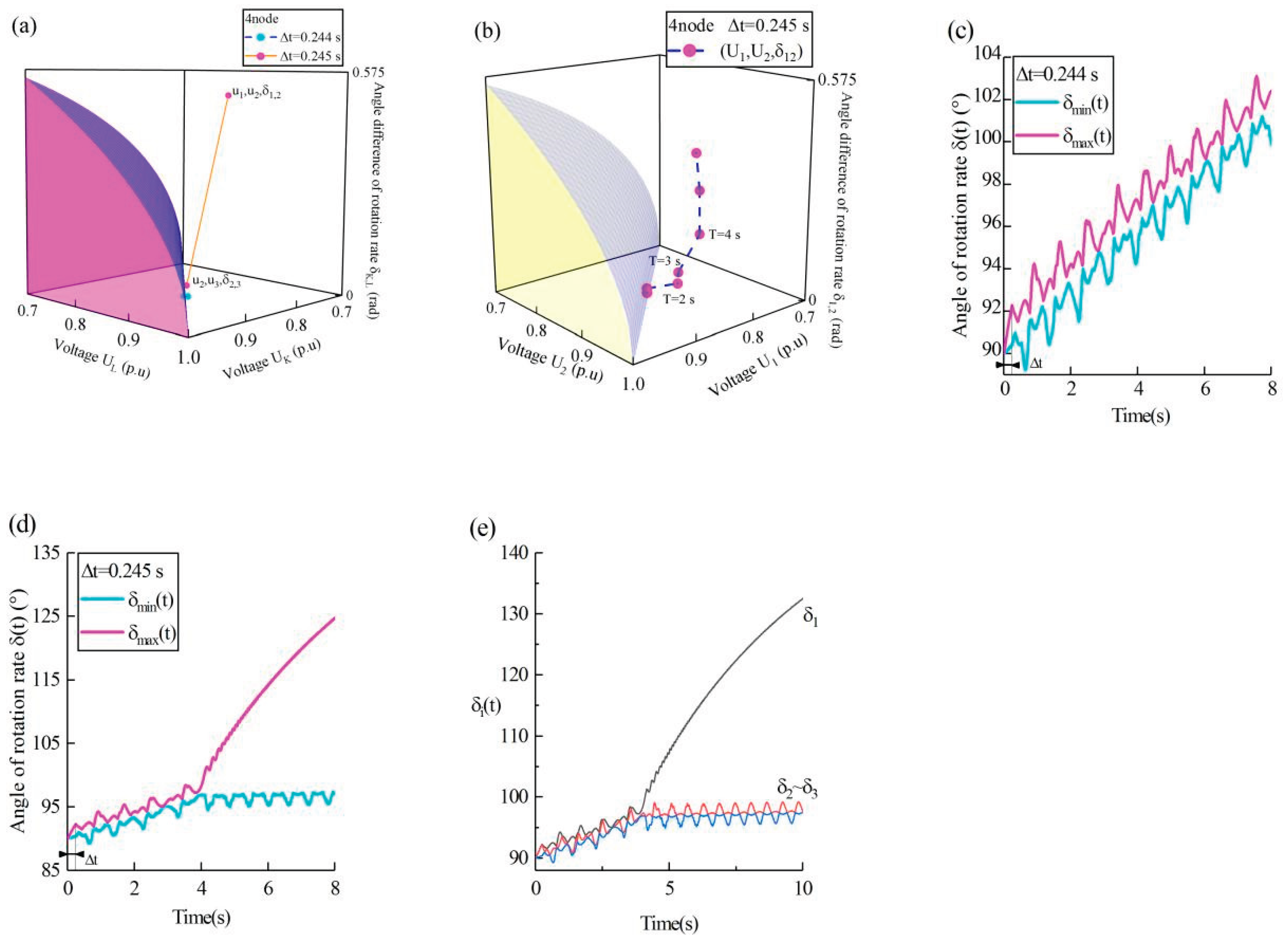
A three-phase short circuit to a ground fault occurred at the 4-node. The values of ${\delta }_i(t)$ are calculated using simulation software and Equation (2). $(u_K,u_L,{\delta }_{K,L})$ are calculated using Equations (3) and (4).

(a). Synchronization stabilization discrimination and partial synchronization. When $\Delta t=0.244 s$, two cyan dots are clustered at the boundary. When $\Delta t=0.245 s$, $\left(u_1,u_2,{\delta }_{1,2}\right)$ is outside the boundary and away from $(u_2,u_3,{\delta }_{2,3})$ (magenta dots).

(b). The stability of multiple swings for multiple generators. $\Delta t=0.245 s$. $\left(u_1,u_2,{\delta }_{1,2}\right)$ crosses the boundary outwardly in the time interval $\left(2 s, 3 s\right)$ and ${\delta }_{1,2}$ rapidly increases in the time interval $\left(4 s, 5 s\right)$. This is in good agreement with the result presented in Figure 3(d). $dT=1s$.

(c) and (d) show experimental verification of synchronous stability and the stability of multiple swings for multiple generators. The horizontal axis represents the time. The vertical axis represents the value of ${\delta }_i(t)$. The maximum value of ${\delta }_i(t)$ is represented by the magenta curve and the minimum value is represented by the cyan curve. At 8 s, ${\delta }_{\max }(t)-{\delta }_{\min }(t)\approx 3°$ in (c), and ${\delta }_{\max }(t)-{\delta }_{\min }(t)\approx 28°$ in (d). Meta-generators are synchronized at $\Delta t=0.244 s$ and out-of-sync at $\Delta t=0.245 s$.

(e).The phenomenon of partial synchronization. ($\Delta t=0.245s$). The horizontal axis represents the time. The vertical axis represents the value of ${\delta }_i(t)$. In the early stages, all meta-generators are synchronized. After approximately 4 s, meta-generator 1 disengages from the cluster (black line). Meta-generators 2 ~ 3 form a synchronized cluster (red line and blue line). Three meta-generators break up into two coherent groups.

The straightforward method to prove that “the boundary is independent of the network” is to test whether Equation (10) holds true for a completely different network. Analogous results were obtained for the 3-generator test system using the same procedure (see Figure 3). Figure 2 shows the results of the simulation with the New England test system, whereas the results in Figure 3 are from the 3-generator test system. The New England test system and 3-gen are two completely different network systems [26,27]. They clearly have completely different topology and parameters, but in both cases, the same boundary equation is applied. This is because the aforementioned evidence can be reproduced in the 3-generator test system. Both Figure 3(a) and Figure 2(b) correspond to evidence 1) mentioned above. Both Figure 3(b) and Figure 2(c) correspond to evidence 2). Both Figure 3(e) and Figure 2(f) correspond to evidence 3). Consequently, a comparison of Figure 2 and Figure 3 reveals that Equation (10) can be used to characterize the boundary of a different network. Moreover, the failures occurring on different network nodes can lead to different results. The results in Figure S5 and Table S1 correspond to different failures. These findings demonstrate that the synchronization stability boundary is is not only independent of the network topology, it is also independent of system parameters and fault locations. All of the above evidence suggests that in complex systems, synchronization conditions can be defined by the behavior of individuals, regardless of whether or not there is a clear network of interactions between those individuals.

More information can be obtained from the expression of Equation (10). Specifically, the left-hand side of Equation (10) represents the global stability domain [20] (i.e.,when $\left|u_K\right|=\left|u_L\right|$,$\forall {\delta }_{K,L}\ge 0,P_{\Delta u}=P_{\partial u}$).

$$\left|u_K\right|=\left|u_L\right|$$

(16)

is a manifestation of the symmetry of the system. This finding shows that high symmetry can promote synchronization in complex networks. This can explain why symmetric networks have better synchronization capabilities. This has been reported in various studies [36,37].

The right-hand side of Equation (10) has a variant that is expressed by:

$${\delta }_{K,L}^{cr}=\arccos (1-{\displaystyle \frac{\left|u_K\right|-\left|u_L\right|}{2\left|u_K\right|}})$$

(17)

where ${\delta }_{K,L}^{cr}$ is the stability margin of the Kth and Lth meta-generator angle difference of the rotation rate. That is, for $(u_K,u_L,{\delta }_{K,L})$, the system remains synchronously stable when ${\delta }_{K,L}^{cr}>{\delta }_{K,L}$. The difference between $\left|u_K\right|$ and $\left|u_L\right|$ can be used to measure the degree of asymmetry of the system. When $\left|u_K\right|,\left|u_L\right|$ are sufficiently close [38], ${\delta }_{K,L}^{cr}$ tends to 0. As $\left|u_K\right|-\left|u_L\right|$ increases, ${\delta }_{K,L}^{cr}$ increases. In other words, the synchronization stability domain becomes larger as the degree of asymmetry increases. This explains the recently discovered superior synchronization stability of highly asymmetric systems [25,39]. It is very difficult to maintain a high degree of symmetry at all times after the system is perturbed. For those systems requiring stability, asymmetry may be a more economical candidate. In addition, Equation (17) shows the potential for stability control: we may be able to increase the synchronization stability margin by carefully controlling the voltage. When ${\delta }_{K,L}>{\displaystyle \frac{\pi }{3}}$, the Kth and Lth meta-generators are not synchronized. The synchronization stability domain is finite.

Consequently, both high symmetry and high asymmetry promote synchronization. The expression of Equation (10) is very simple, yet it harmonizes these two contradictory conclusions well and requires no additional assumptions.

In summary, Equation (10) enables a unified analysis of the synchronization stability of the grid and provides a new understanding of synchronization. To determine the stability of n oscillators, only n pairs of variables $u_i,{\delta }_i,i\in (1,2,\dots ,n)$ are required. These variables can be readily obtained. Compared to the current literature [40,41,42], the conclusions of this paper may indicate that we need to revisit the relationship between synchronization phenomena and networks.

3.2. Spontaneous Synchronization in Power System

Power systems may be destabilized when they are disturbed [43]. Therefore, it is equally important to study the the transition behavior of a disturbed system from stable to unstable states. Observation shows that when the system is disturbed and on the brink of destabilization, the trajectory of ${\delta }_i$ becomes intriguing. A surprisingly specific structure emerges from the collective behavior of these trajectories. The polar coordinates of the ith meta-generator are denoted by $（u_i,{\delta }_i)$.

Figure 4. Spontaneous synchronization positions and unique structure. (Meta-generators in the 10-gen).

Figure 4. Spontaneous synchronization positions and unique structure. (Meta-generators in the 10-gen).

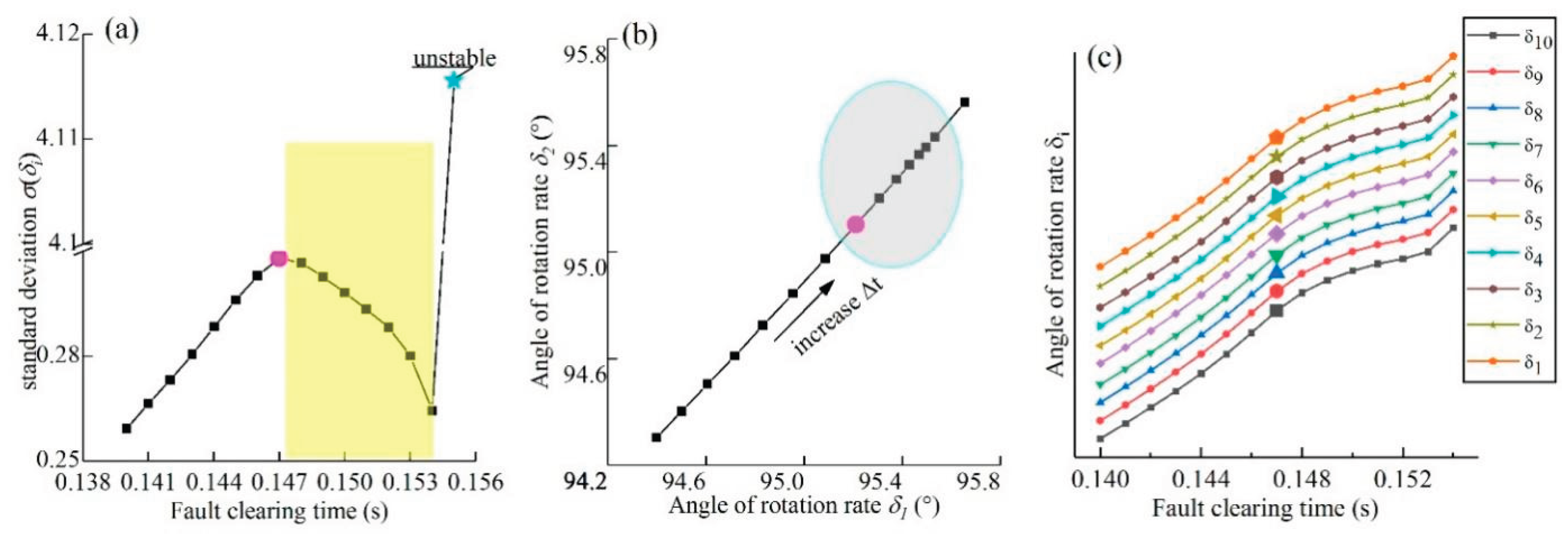
The fault clearing time $\Delta t$ increases from 0.140 s to 0.155 s. The arrow means the direction of increase in $\Delta t$ (the 18-node three-phase short circuit to the ground fault). $d(\Delta t)=0.001 s$. The data of ${\delta }_i(t)$ are derived from numerical simulations experiments and ${\delta }_i$ are calculated using Equation (3).

(a). Spontaneous synchronization of meta-generators. The horizontal axis represents the fault clearing time. The vertical axis represents the standard deviation of $\delta$. The yellow area means the thin layer where spontaneous synchronization occurs. Here, $\sigma \left({\delta }_i\right)$ denotes the standard deviation of $\delta$, which begins to decrease at 0.147 s (magenta dots) and increases by 1300% at 0.155 s when the system becomes unstable (cyan pentagram dots). $\sigma \left({\delta }_i\right)$ can be calculated using Equation (6).

(b). The phenomenon of potential barrier on plane ${\delta }_1-{\delta }_2$. $\Delta t$ increased from 0.140 s to 0.154 s. The black arrow means the direction in which $\Delta t$ increased. From $\Delta t=0.147 s$ (the magenta dot) onward, the distance between neighboring points decreased in the direction of the black arrow (the elliptical shaded area).[For the sake of image clarity, the point corresponding to $\Delta t=0.155 s$ is difficult to display in the figure; its data can be found in doi.org/10.57760/sciencedb.24825.]

(c). Starting points of spontaneous synchronization and long-range correlation. The horizontal axis represents the fault clearing time. The amplified points mean the starting points of spontaneous synchronization. Near the boundary, all of starting points appear at $\Delta t=0.147 s$. The trends of all of ${\delta }_i$ were almost identical. Combining (b) and (c) reveals that in this case, unique structures exist between any two meta-generators.[Since the values of ${\delta }_i$ corresponding to the same $\Delta t$ are nearly identical, the scale values on the vertical axis had to be omitted to illustrate the trend and facilitate visualization. This data can be found in doi.org/10.57760/sciencedb.24825, as shown in “Data availability”.]

As shown in Figure 4(a), $\sigma \left({\delta }_i\right)$ exhibits discontinuity at 0.154 s and 0.155 s. In agreement with the findings presented in Figure 2, the system is stable at $\Delta t=0.154 s$ and unstable at $\Delta t=0.155 s$. The decrease in $\sigma \left({\delta }_i\right)$ from the highest point in the yellow region indicated that on the brink of destabilization, the velocity of the subsystem was spontaneously directed toward the mean value. This counterintuitive phenomenon is consistent with the definition of spontaneous synchronization effect [13,44]. It can be inferred that the spontaneous synchronization effect causes $\sigma \left({\delta }_i\right)$ to decrease whether the system crosses the yellow area(in Figure 4(a)) in the inward or outward direction. Therefore, within the thin layer, the results of $\sigma \left({\delta }_i\right)$ in different directions are not the same. Moreover, Referring to Figure S3(b), the fault clearing time at $(u_K,u_L,{\delta }_{K,L})$ within the thin layer aligns with the fault clearing time corresponding to the yellow-shaded region in Figure 4(a). This indicates that the system undergoes self-organization before losing synchronous stability, and this phenomenon occurs at the boundary of synchronous stability. For power systems, the spontaneous synchronization that occurs prior to destabilization provides additional protection for the synchronous stability of the system.

As shown in Figure 4(b), for a constant step size $d(\Delta t)=0.001 s$, the interval between points decreases progressively within the shaded area, leading to the emergence of a unique trajectory structure. This novel structure, termed a “potential barrier”, exhibits “decelerating motion” within the shaded area, as if the mass points were crossing a potential barrier. To the best of my knowledge, this structure has not been previously reported. $\sigma \left({\delta }_i\right)$ reaches its maximum at $\Delta t=0.147 s$ and begins to decrease in Figure 4(a). The magenta dot corresponds exactly to $\Delta t=0.147 s$ in Figure 2(b).

All of amplified points appear at the identical $\Delta t$ in Figure 4(c). These amplified points are located at the transition of ${\displaystyle \frac{d^2{\delta }_i}{d{(\Delta t)}^2}}$. Specifically, at $\Delta t=0.147 s$, ${\displaystyle \frac{d^2{\delta }_i}{d{(\Delta t)}^2}}$ of all meta-generators transforms simultaneously. Prior to this, ${\displaystyle \frac{d^2{\delta }_i}{d{(\Delta t)}^2}}>0$. After this, ${\displaystyle \frac{d^2{\delta }_i}{d{(\Delta t)}^2}}<0$. Moreover, the system is unstable at $\Delta t=0.155 s$. These results demonstrate that $\Delta t=0.147 s$ is the starting point and $\Delta t=0.154 s$ is the end of spontaneous synchronization. This is the position of spontaneous synchronization where emergence occurs. Self-organizing behavior emerges from the interactions of these meta-generators, and its effects are reflected in the behavior of the oscillators. Given that these meta-generators are connected to different nodes, this result suggests that they exhibit long-range correlation at the point of impending destabilization. This correlation leads to a collective movement of all individuals as a whole.

In contrast to the previous literature discussing synchronization in power grids [11,22], this work reports a new phenomenon of spontaneous synchronization. These phenomena may originate from different mechanisms, since they occur in forward processes subject to perturbations, exhibit a special structure. Simultaneously, the thin layer where spontaneous synchronization occurred is found close to the synchronization stability boundary. That is, oscillators in the same network may have two different spontaneous synchronization behaviors at the same time.

Currently, spontaneous synchronization is considered to be closely related to the network structure [45]. However, the results of this section yield another conclusion. Similar to Figure 4(a), those results in Figure S4 from different fault responses suggest that the system suddenly self-organizes toward synchronous evolution only when it about to reach the edge of synchronous stable. These phenomenon can be interpreted as spontaneous synchronization ‌occurring only close to the synchronous stability boundary. Consequently, for coupled network systems, the link between spontaneous synchronization and the boundary suggests that the location where spontaneous synchronization occurs is constrained by Equation (10). This finding suggests that spontaneous synchronization is independent of the network. As shown in Figure S1, results from entirely different network (the 3-generator test system) further corroborate this conclusion. This conclusion challenges the traditional perception of spontaneous synchronization in networks.

More importantly, these unexpected results show that we still lack research on the destabilization process of complex systems and the interaction and behavior of oscillators at the stability boundary. The behavior of the systems near the boundary is diverse. For example, A comparison of Figures 4 and S1 reveals that spontaneous synchronization can result in at least two different results. The reasons for this difference, or rather, the specific conditions for the formation of a potential barrier, require further research. Moreover, the thin layer where spontaneous synchronization occurs has some thickness. However, the solution for this thickness is not clear. These issues will be addressed in future research.

4. Conclusions

This research has broad implications. Although the derivation of the boundary equation is heuristic, mathematical proofs and simulation results provide strong evidence for this equation. In this paper, the analysis of cluster synchronization is simplified, the contradiction of different symmetries promoting synchronization is reconciled and a new phenomenon of spontaneous synchronization is reported. These broaden our understanding of synchronization phenomena. While existing research on synchronization in complex networks predominantly relies on network models, this work demonstrates that the synchronization boundary and spontaneous synchronization are actually determined by individual behavior rather than system parameters and network structure. This finding challenges traditional perspectives on synchronization phenomena and may open new research directions across disciplines.

Furthermore, as an application of synchronization of complex networks in real power grids, this study derives and proves a unified synchronization stability boundary that combines theoretical innovation with engineering practicality. The boundary is described only by the parameters u,w and is independent of the topology and impedance of the grid, as well as of the parameters of the generator (e.g., damping and inertia). These features grant it great flexibility. Compared to conventional methods, this approach requires only the voltage and rotor speed as ultra-simplified criteria, significantly reducing the complexity of stability analysis. The approach can also be directly applied to the case of multiple swings for multiple generators and generator coherent groups, which is validated in different networks and conforms well to numerical experiments. Together with strategies such as virtual synchronous generators, it is also suitable for the synchronization stability discrimination of renewable energy grids with unknown parameters, time-varying topology and no physical rotation. Instead, we can determine the amount of inertia needed for a renewable energy grid based on the stability margin. This may be a new solution for future adaptive grid control measures.

References

- Koronovskii, A.A., Moskalenko, O.I., and Hramov, A.E. (2012). synchronization in complex networks. Tech. Phys. Lett. 38, 924–927. [CrossRef]
- Dörfler, F., Chertkov, M., and Bullo, F. (2013). Synchronization in complex oscillator networks and smart grids. Proc. Natl. Acad. Sci. U. S. A. 110, 2005–2010. [CrossRef]
- Shi, Di., Lü, L., and Chen, G. (2019). Totally homogeneous networks. Natl. Sci. Rev. 6, 962–969. [CrossRef]
- Wu, K., Hao, X., Liu, J., Liu, P., and Shen, F. (2022). Online Reconstruction of Complex Networks From Streaming Data. IEEE Trans. Cybern. 52, 5136–5147. [CrossRef]
- Linyuan, L.L., and Zhou, T. (2011). Link prediction in complex networks: A survey. Phys. A Stat. Mech. its Appl. 390, 1150–1170. [CrossRef]
- Xu, Y., Zhou, W., and Fang, J. (2012). Topology identification of the modified complex dynamical network with non-delayed and delayed coupling. Nonlinear Dyn. 68, 195–205. [CrossRef]
- Meena, C., Hens, C., Acharyya, S., Haber, S., Boccaletti, S., and Barzel, B. (2023). Emergent stability in complex network dynamics. Nat. Phys. 19, 1033–1042. [CrossRef]
- Dörfler, F., and Bullo, F. (2012). Synchronization and transient stability in power networks and nonuniform Kuramoto oscillators. SIAM J. Control Optim. 50, 1616–1642. [CrossRef]
- Watts, D.J., and Strogatz, S.H. (1998). Collective dynamics of “small-world” networks. Nature 393, 440–442. [CrossRef]
- Barahona, M., and Pecora, L.M. (2002). Synchronization in Small-World Systems. Phys. Rev. Lett. 89, 54101. [CrossRef]
- Strogatz, S.H. (2003). Sync: The Emerging Science of Spontaneous Order (Hyperion).
- Wang, B., Fang, B., Wang, Y., Liu, H., and Liu, Y. (2016). Power System Transient Stability Assessment Based on Big Data and the Core Vector Machine. IEEE Trans. Smart Grid 7, 2561–2570. [CrossRef]
- Zhu, L., and Hill, D.J. (2020). Synchronization of Kuramoto Oscillators: A Regional Stability Framework. IEEE Trans. Automat. Contr. 65, 5070–5082. [CrossRef]
- Xu, Z., Li, X., and Duan, P. (2020). Synchronization of complex networks with time-varying delay of unknown bound via delayed impulsive control. Neural Networks 125, 224–232. [CrossRef]
- Yang, P., Liu, F., Wei, W., and Wang, Z. (2022). Approaching the Transient Stability Boundary of a Power System: Theory and Applications. IEEE Trans. Autom. Sci. Eng., 1–12. [CrossRef]
- Nian, F. (2012). Adaptive coupling synchronization in complex network with uncertain boundary. Nonlinear Dyn. 70, 861–870. [CrossRef]
- Chiang, H.D., Wu, F.F., and Varaiya, P.P. (1994). A BCU Method for Direct Analysis of Power System Transient Stability. IEEE Trans. Power Syst. 9, 1194–1208. [CrossRef]
- Al-Ammar, E.A., and El-Kady, M.A. (2010). Application of operating security regions in power systems. IEEE PES Transm. Distrib. Conf. Expo. Smart Solut. a Chang. World. [CrossRef]
- Wu, X., Xi, K., Cheng, A., Lin, H.X., and van Schuppen, J.H. (2023). Increasing the synchronization stability in complex networks. Chaos 33. [CrossRef]
- Yu, Y., Liu, Y., Qin, C., and Yang, T. (2020). Theory and Method of Power System Integrated Security Region Irrelevant to Operation States: An Introduction. Engineering 6, 754–777. [CrossRef]
- Rimorov, D., Wang, X., Kamwa, I., and Joos, G. (2018). An approach to constructing analytical energy function for synchronous generator models with subtransient dynamics. IEEE Trans. Power Syst. 33, 5958–5967. [CrossRef]
- Motter, A.E., Myers, S.A., Anghel, M., and Nishikawa, T. (2013). Spontaneous synchrony in power-grid networks. Nat. Phys. 9, 191–197. [CrossRef]
- Li, X., Wei, W., and Zheng, Z. (2023). Promoting synchrony of power grids by restructuring network topologies. Chaos An Interdiscip. J. Nonlinear Sci. 33, 63149. [CrossRef]
- Smith, O., Coombes, S., and O’Dea, R.D. (2024). Stability Analysis of Electrical Microgrids and Their Control Systems. PRX Energy 3, 1. [CrossRef]
- Molnar, F., Nishikawa, T., and Motter, A.E. (2021). Asymmetry underlies stability in power grids. Nat. Commun. 12, 1–9. [CrossRef]
- Anderson, P.M., and Fouad, A.A. (2008). Power system control and stability (John Wiley & Sons).
- Pai, A. (1989). Energy function analysis for power system stability (Springer Science & Business Media).
- Wu Zhongxi, and Zhou Xiaoxin Power System Analysis Software Package (PSASP)-an integrated power system analysis tool. In POWERCON ’98. 1998 International Conference on Power System Technology. Proceedings (Cat. No.98EX151) (IEEE), pp. 7–11. [CrossRef]
- Casals, M.R., Bologna, S., Bompard, E.F., D’, G., Agostino, N.A., Ellens, W., Pagani, G.A., Scala, A., and Verma, T. (2015). Knowing power grids and understanding complexity science. Int. J. Crit. Infrastructures 11, 4. [CrossRef]
- Kuramoto, Y., and Battogtokh, D. (2002). Coexistence of Coherence and Incoherence in Nonlocally Coupled Phase Oscillators. Physics (College. Park. Md). 4, 380–385. [CrossRef]
- Cho, Y.S., Nishikawa, T., and Motter, A.E. (2017). Stable Chimeras and Independently Synchronizable Clusters. Phys. Rev. Lett. 119. [CrossRef]
- Fan, H., Kong, L.W., Wang, X., Hastings, A., and Lai, Y.C. (2021). Synchronization within synchronization: Transients and intermittency in ecological networks. Natl. Sci. Rev. 8, 0–9. [CrossRef]
- Sorrentino, F., Pecora, L.M., Hagerstrom, A.M., Murphy, T.E., and Roy, R. (2016). Complete characterization of the stability of cluster synchronization in complex dynamical networks. Sci. Adv. 2, 1–8. [CrossRef]
- Ajala, O., Dominguez-Garcia, A., Sauer, P., and Liberzon, D. (2019). A Second-Order Synchronous Machine Model for Multi-swing Stability Analysis. 51st North Am. Power Symp. NAPS 2019. [CrossRef]
- Alberto, L.F.C., and Bretas, N.G. (2000). Required damping to assure multiswing transient stability: the SMIB case. Int. J. Electr. Power Energy Syst. 22, 179–185. [CrossRef]
- Pecora, L.M., Sorrentino, F., Hagerstrom, A.M., Murphy, T.E., and Roy, R. (2014). Cluster synchronization and isolated desynchronization in complex networks with symmetries. Nat. Commun. 5. [CrossRef]
- Denker, M., Timme, M., Diesmann, M., Wolf, F., and Geisel, T. (2004). Breaking Synchrony by Heterogeneity in Complex Networks. Phys. Rev. Lett. 92, 1–4. [CrossRef]
- Karatekin, C.Z., and Uçak, C. (2008). Sensitivity analysis based on transmission line susceptances for congestion management. Electr. Power Syst. Res. 78, 1485–1493. [CrossRef]
- Nishikawa, T., and Motter, A.E. (2016). Symmetric States Requiring System Asymmetry. Phys. Rev. Lett. 117, 114101. [CrossRef]
- Holland, M.D., and Hastings, A. (2008). Strong effect of dispersal network structure on ecological dynamics. Nature 456, 792–794. [CrossRef]
- Chen, G. (2022). Searching for Best Network Topologies with Optimal Synchronizability: A Brief Review. IEEE/CAA J. Autom. Sin. 9, 573–577. [CrossRef]
- Nishikawa, T., Sun, J., and Motter, A.E. (2017). Sensitive dependence of optimal network dynamics on network structure. Phys. Rev. X 7, 1–21. [CrossRef]
- Scheffer, M., Carpenter, S.R., Lenton, T.M., Bascompte, J., Brock, W., Dakos, V., Van De Koppel, J., Van De Leemput, I.A., Levin, S.A., Van Nes, E.H., et al. (2012). Anticipating critical transitions. Science (80-. ). 338, 344–348. [CrossRef]
- Dörfler, F., and Bullo, F. (2014). Synchronization in complex networks of phase oscillators: A survey. Automatica 50, 1539–1564. [CrossRef]
- Fan, H., Wang, Y., and Wang, X. (2023). Eigenvector-based analysis of cluster synchronization in general complex networks of coupled chaotic oscillators. Front. Phys. 18. [CrossRef]
Disclaimer/Publisher’s Note: The statements, opinions and data contained in all publications are solely those of the individual author(s) and contributor(s) and not of MDPI and/or the editor(s). MDPI and/or the editor(s) disclaim responsibility for any injury to people or property resulting from any ideas, methods, instructions or products referred to in the content. |
© 2025 by the authors. Licensee MDPI, Basel, Switzerland. This article is an open access article distributed under the terms and conditions of the Creative Commons Attribution (CC BY) license (http://creativecommons.org/licenses/by/4.0/).
Copyright: This open access article is published under a Creative Commons CC BY 4.0 license, which permit the free download, distribution, and reuse, provided that the author and preprint are cited in any reuse.