
Submitted:
09 April 2025
Posted:
10 April 2025
You are already at the latest version
Abstract
We investigate the stochastic disruption of synchronization patterns in a system of two non-identical Rulkov neurons coupled via an electrical synapse. By analyzing the system deterministic dynamics, we identify regions of mono-, bi-, and tristability, corresponding to distinct synchronization regimes as a function of coupling strength. Introducing stochastic perturbations to the coupling parameter, we explore how noise influences synchronization patterns, leading to transitions between different regimes. Notably, we find that increasing noise intensity disrupts lag synchronization, resulting in intermittent switching between a synchronous 3-cycle regime and asynchronous chaotic states. This intermittency is closely linked to the structure of chaotic transient basins, and we determine a noise intensity range in which such behavior persists, depending on the coupling strength. Using both numerical simulations and an analytical confidence ellipse method, we provide a comprehensive characterization of these noise-induced effects. Our findings contribute to the understanding of stochastic synchronization phenomena in coupled neuronal systems and offer potential implications for neural dynamics in biological and artificial networks.
Keywords:
Rulkov map
; neuronal model
; coupled neurons
; nonlinear dynamics
; chaos
; noise
; intermittency
; synchronization
1. Introduction
In neuronal networks, synchronization plays a crucial role in information processing, neural coding, and motor control, and its disruption has been implicated in various neurological disorders such as epilepsy, Parkinson’s disease, and schizophrenia [1,2,3,4]. Real-world neuronal networks are subject to stochastic fluctuations arising from intrinsic neural noise, synaptic variability, and external perturbations [5,6,7,8]. These fluctuations can significantly impact neuronal dynamics, leading to intermittent synchronization, chaotic transitions, and complete desynchronization [9,10,11]. In multistable systems, noise can lead to switching between coexisting attractors resulting in multistate intermittency and monostability [12,13,14,15]. Therefore, studying the stability and stochastic disruption of synchronization in coupled neurons is of great theoretical and practical significance.
In this work, we are interested in how random perturbations of the coupling parameter affect synchronization patterns in a coupled neural system. As a neural model, we consider a system of two non-identical Rulkov neurons coupled by an electrical synapse [16]. The Rulkov model is widely used to describe the bursting dynamics of neurons due to its computational efficiency and ability to capture key aspects of neuronal excitability. Various phenomena in the isolated deterministic and stochastic Rulkov model are actively studied (see, e.g. [17,18,19,20]).
Coupled Rulkov neurons exhibit rich dynamical behaviors, including multiple synchronization regimes that depend on the coupling strength and system parameters [21,22,23,24,25]. Depending on the coupling parameter, different synchronization states, including mono-, bi-, and tristable regimes, can emerge, corresponding to distinct synchronization patterns such as in-phase and lag synchronization. Through systematic parametric analysis, we identify key conditions under which noise intensity influences the transitions between different dynamical states. To analyze these complex dynamics, we employ a combination of direct numerical simulations and an analytical method based on confidence domains, which provide a robust statistical tool for assessing the variability of system trajectories under stochastic perturbations, allowing us to characterize the range of noise intensity that sustains intermittency and determine its dependence on coupling strength. The size and shape of the confidence domains are determined from the stochastic sensitivity matrices of the corresponding deterministic attractors. The stochastic sensitivity function technique was elaborated for different types of regular and chaotic attractors [26] and is now actively used in the parametric analysis of various stochastic phenomena (see, e.g. [23,27,28]).
A particularly intriguing phenomenon observed in our study is the existence of an intermittency regime, where a synchronous 3-cycle regime is interrupted by asynchronous chaotic bursts. This phenomenon underscores the critical role of basins of chaotic transients in shaping the response of the system to stochastic perturbations. The presence of intermittent chaotic behavior suggests that noise can induce transitions between metastable states, highlighting the nontrivial interplay between deterministic and stochastic influences in coupled neuronal dynamics. We investigate the stochastic disruption of lag synchronization and the emergence of a monostable in-phase synchronization regime.
The rest of this paper is organized as follows: Section 2 introduces the deterministic model of coupled Rulkov neurons and explores their dynamical behavior. Section 3 extends the discussion to the stochastic model, highlighting synchronization regimes and scenarios of stochastic disruption. In Section 4, we analyze intermittent chaotic behavior in detail. Finally, Section 5 summarizes our findings and discusses potential directions for future research.
2. Deterministic Model
Consider a system of two non-identical neurons modeled by the Rulkov map [16] and mutually coupled by electrical synapses:
Here, In system (1), where is a mismatch parameter. The parameter regulates the strength of coupling.
2.1. Dynamics of isolated neuron
Figure 1 shows the -interval in which the isolated neuron demonstrates the transformation of a stable 3-cycle into a chaotic attractor when passes the crisis bifurcation point This transition from order to chaos is justified by the largest Lyapunov exponent in the bottom panel.
2.2. Dynamics of coupled neurons
Now, consider now the corporative dynamics of the coupled system (1) with and , i.e., . While isolated neurons with these parameters exhibit 3-cycles, the joint dynamics is governed by the coupling parameter , as illustrated in Figure 2, which presents the bifurcation diagram of the x variable.
At weak coupling strengths, the system (1) exhibits tristability, with three coexisting 3-cycles: (blue), (green), and (orange). These attractor and their basins of attraction are illustrated in Figure 3 for different values of the coupling parameter .
Figure 3(a) illustrates the coexistence of three 3-cycles at . As the coupling increases, cycle is annihilated, reducing system (1) to a bistable state with two coexisting 3-cycles, and , at (Figure 3(b)). A further increase in eliminates cycle , making the system monostable with a single remaining attractor, cycle , at (Figure 3(c)). Finally, at the crisis bifurcation occurring at , cycle loses stability, causing the system transition into chaos. The resulting chaotic attractor is shown in Figure 3(d) for .
The cycles , , and correspond to different synchronization patterns. Solutions originating from the basins of and exhibit synchronization in a one-step shift mode. In the basin of , solutions stabilize to a 3-cycle where the y-coordinate is one step ahead of the x-coordinate, which we denote as the synchronization mode. Conversely, in the basin of , solutions stabilize to a 3-cycle for where the y-coordinate lags one step behind the x-coordinate, referred to as the synchronization mode. Finally, solutions in the basin of stabilize to a 3-cycle without any coordinate shift, denoted as the synchronization mode. Thus, as the coupling increases, the system first losses the synchronization mode, followed by the synchronization mode.
3. Stochastic Model
Let us now study how noise influences system (1). The dynamics of the coupled neurons under random fluctuations in the coupling parameter, , is governed by the following equations:
Here, represents uncorrelated white Gaussian noise with intensity .
Next, we analyze how the solutions of system (2) depend on the noise intensity .
3.1. Stochastic Deformations in the Tristability Case
First, consider system (2) with . As shown in the previous section, at this coupling strength, the deterministic system (1) exhibits the coexistence of three 3-cycles (, , and ) , as illustrated in Figure 3(a).
Figure 4 demonstrates how stochastic perturbations in the coupling parameter influence the system dynamics. In Figure 4(a,b,c), we plot the evolution of the difference between the x- and y-coordinates () of solutions, corresponding to cycles (orange), (green), and (blue) under three different noise intensity values.
For weak noise (), stochastic solutions of system (2) that start at cycles or remain in these cycles, as shown in upper two panels of Figure 4(a). However, trajectories that begin at cycle eventually switch to either cycle or after a transient period, as illustrated in lower two panels. Thus, weak noise disrupt cycle while leaving the other cycles unaffected.
As shown in Figure 4(b), stronger noise () not only eliminates cycle (lowest panel) but also destroys cycle (middle panel) while cycle remains unaffected (upper panel). Interestingly, solutions that start at (middle panel) exhibit mutual transitions between and (), eventually stabilizing near cycle . Meanwhile, solutions originating from undergo sequential transitions . Thus, regardless of the initial conditions, all transitions at this noise level ultimately lead to cycle , making the system monostable.
When the noise intensity increases to , all three cycles lose stability. At this noise level, each cycle is disrupted by chaotic bursts, as shown in Figure 4(c). The system undergoes the following stochastic transitions: , , and . Thus, regardless of the initial state, the stochastic system (2) transitions into an intermittent regime characterized by alternating small-amplitude stochastic oscillations near and large-amplitude chaotic oscillations . Random states of this chaotic regime are depicted in Figure 4(d).
Figure 5 illustrate the stochastic transformations the () variable as the noise intensity gradually increases, starting from deterministic cycles (Figure 5(a)), (Figure 5(b)), and (Figure 5(c)). These cycles are shown in the background in light colors. Colored dots represent the random states of system (2) for solutions , , and , plotted after 1000 transient steps. The color of these dots matches the corresponding starting cycle but appears in a brighter shade.
For weak noise, the random solutions remain close to their respective starting cycles. However, as the noise intensity increases, stochastic switches between coexisting states begin to appear, as shown in the time series in Figure 4(a,b). These transitions are revealed in Figure 5 as dots between horizontal lines.
In the case of (Figure 5(a)), these transitions disrupt the synchronization mode. As the noise intensity increases further, random states begin clustering around cycle (see the time series in Figure 4(b)). This indicates that both the and synchronization modes are destroyed, leaving only the synchronization mode intact. When the noise becomes sufficiently strong, solutions starting at transition directly into the intermittent regime , characterized by alternating small-amplitude stochastic oscillations near and large-amplitude chaotic oscillations (see the time series and random states in Figs. Figure 4(c,d)). Consequently, the synchronization mode is temporarily disrupted by random disturbances.
Stochastic transformations of solutions starting from the 3-cycle are shown in Figure 5(b). For noise intensities up to , these solutions remain localized near the deterministic cycle. At , stochastic transformations following the sequence are observed, as illustrated in the time series in Figure 4(b) (green trace). For stronger noise, the stochastic system transits to the regime (see the time series shown in green in Figure 4(c) for ). For solutions starting at the 3-cycle , only a single-stage stochastic transformation occurs, where noisy oscillations near transition into the intermittent mode (see the orange time series in Figure 4(c) for ).
To summarize the effect of noise in the tristability case, increasing noise intensity first destroys cycle , followed by the destruction of cycle , leaving cycle as the most resilient to noise.
3.2. Confidence Domain Method
The cycle breakdown process described above can be analyzed analytically using the confidence domain method [26], where the mutual arrangement of confidence domains and attractors’ basins of attraction plays a key role. Below, we briefly present details of the confidence domain method.
Consider a deterministic system with an exponentially stable 3-cycle consisting of successive states , , and . Under random disturbances, the stochastic sensitivity of these states is determined by the corresponding matrices , , and . These matrices satisfy the following algebraic equations [26]:
Here, is the Jacobi matrix at the point of the 3-cycle, while the matrices characterize the stochastic disturbances.
For system (2), the matrix is given by
The stochastic sensitivity matrix satisfies the matrix equation
where The other stochastic sensitivity matrices, and , can be determined using the recurrence relations provided earlier.
These stochastic sensitivity matrices are useful for approximating the dispersion of random states around the points of the deterministic 3-cycle. This approximation is represented in the form of confidence ellipses. For each state of the 3-cycle, the confidence ellipses are defined as
Here, are the coordinates of the ellipse in the basis of normalized eigenvectors of the matrix , while are the corresponding eigenvalues. The parameter P represents the fiducial probability.
In Figure 6, we present magnified fragments of the phase plane of the deterministic system (1), highlighting the basins of attraction near specific states of the 3-cycles. The basin points are color-coded: light blue for cycle , light green for cycle , and white for cycle . A notable feature of these basins is the distinction between solid and fractal parts. The solid region surrounds the cycle points, while outside tis area, the basins of all three 3-cycles are fractally interwoven.
In addition to these deterministic basins, Figure 6 also displays confidence ellipses for the stochastic system (2). As the noise intensity increases, these ellipses expand in size. As long as the a confidence ellipse remains within the solid region of a basin, no transitions occur. However, once the ellipse extends beyond the solid part and overlaps with the fractal region, it begins to encompass points from the basins of other coexisting attractors. This expansion marks the breakdown of the initial oscillatory regime and signals transitions to alternative oscillatory modes.
Now, let us examine how the confidence domain method applies in the case of tristability.
In Figure 6(a), confidence ellipses are plotted around a point of cycle for two noise intensities: and . For , the ellipse remains entirely within the solid region of the basin, preventing any noise-induced transitions. However, at , the ellipse extends into the fractal region of the basin, leading to the stochastic destruction of oscillations near .
A different scenario is observed near cycle , where noise with is unsufficient to disrupt stochastic oscillations. As shown in Figure 6(b), the confidence ellipse remains fully contained within the solid part of the basin, ensuring stability. The same holds for cycle , as depicted in Figure 6(c). Consequently, a higher noise intensity is required to destabilize cycle . This effect is evident in Figure 6(b), where the confidence ellipse for extends into the fractal region, signaling to onset of stochastic destruction.
For cycle , it remains stable even under stronger noise with (see blue confidence ellipse in Figure 6(d)). However, as shown in Figure 6(d), when the noise intensity increases to , the confidence ellipse extends into the fractal part of the basin, indicating the breakdown of noisy oscillations near .
Notably, the confidence ellipse method predicts that solutions starting from and transition to at (see Figure 6(a,b)). In contrast, the solutions originating from remain near even up to (see Figure 6(d)). This reveals a broad range of noise intensity, or an "-window", where all solutions of the stochastic system (2) reside near . This finding is supported by the results of numerical simulations presented in Figure 5. Within this -window, regardless of the initial conditions, the synchronization mode persists.
It is worth noting that the predictions made using the confidence ellipse method align well with the results of direct numerical simulations discussed in Section 3.1.
3.3. Stochastic Deformations in the Bistability Case
We now consider system (2) with , which exhibits bistability in the absence of noise, characterized by the coexistence of 3-cycles and (see Figure 3(b)). Possible scenarios of noise-induced transformations in the distribution of random state are shown in Figs. Figure 7(a,b). In Figure 7(a), random states of solutions originating from cycle are shown as a function of noise intensity . A clear transition sequence is observed , indicating the progressive destabilization of the initial cycle as noise increases.
The mutual arrangement of basins and confidence ellipses for (blue) and (red) is illustrated in Figure 7(c). For , the confidence ellipse lies entirely within the solid part of the basin of , meaning that random solutions exhibit only slight fluctuations around . However, for , the ellipse extends into the fractal region of the basin, allowing for noise-induced transitions . The subsequent transition , observed in Figs. Figure 7(a,b), is accurately predicted by the confidence ellipses shown in Figure 7(d).
3.4. Stochastic Deformations in the Monostability Case
Let us now examine the behavior of the stochastic system (2) in the case of monostability, when the original deterministic system (1) possesses only one attractor: the in-phase 3-cycle . This cycle, corresponding to , is shown in Figure 3(c). For this parameter value, the evolution of random states originating from is presented in Figure 8(a) as a function of noise intensity .
As evident from the figure, the 3-cycle demonstrates notable resilience to noise. However, beyond a certain of threshold intensity of , the system (2) undergoes an abrupt change in the probability distribution of its states. Specifically, in Figure 8(b), the random states for (blue) remain tightly clustered near the deterministic cycle , whereas for (orange), the states are broadly scattered across the phase space. This behavior reflects a clear manifestation of noise-induced excitation.
While in the cases of multistability, sharp deformations in the distributions were attributed to noise-induced transitions between coexisting attractors, the mechanism driving the transformation in this monostable case is different. Here, the influence of transient attractors in the underlying deterministic system (1) becomes significant.
4. Transients and Intermittent Synchronization
In this section, we investigate the transient dynamics of the deterministic system (1) and explore noise-induced intermittent synchronization in the corresponding stochastic system (2).
4.1. Short and Long Transients Basins
Although the monostable system (1) with ensures that all trajectories eventually converge to the 3-cycle , the rate of convergence strongly depends on the initial conditions. This behavior is illustrated in Figure 9(a), where initial points of solutions that take more than 200 iterations to converge to with an accuracy of 0.001 are marked in orange. These points define the long transients basin (LTB), while the remaining region—corresponding to faster convergence—is marked in white and referred to as the short transients basin (STB). Notably, the boundary between these basins exhibits a complex, fractal structure. In Figure 9(b), an enlarged fragment of the phase plane is shown near one of the points of 3-cycle , highlighting both the STB and LTB. The STB consists of a solid (white) region and a fractal part, represented by a mixture of white and orange areas. The selected 3-cycle point lies within the solid part of the STB.
We now examine how the transient behavior of solutions to the deterministic system (1) depends on the choice of the initial condition. Specifically, we consider two nearby points, and . Point A lies within the solid part of the STB, whereas point B belongs to its fractal region.
During transients, the system may alternate between synchronous () and asynchronous () states. To quantify these states, we introduce the synchronization index defined as
Note that when the neurons evolve synchronously (i.e., both variables increase or decrease together), and otherwise. Examples of synchronous and asynchronous transients are shown in Figs.Figure 9(c) and Figure 9(d), respectively. Specifically, Figure 9(c) illustrates that the trajectory starting at point A converges to the 3-cycle while maintaining in-phase synchronization (). In contrast, Figure 9(d) shows that the trajectory from point B exhibits a large-amplitude burst with temporary desynchronization, characterized by the interval where .
The diversity of transient behaviors for various initial conditions near point B—located in the fractal region—is illustrated in Figure 9(e). Notably, for , the system exhibits three bursts before ultimately converging to the 3-cycle .
The underlying reason for the noise-induced excitability described above and illustrated in Fig.Figure 8 lies in the presence of a fractal region associated with large-amplitude burst transient attractors in the deterministic system (1). For weak noise, random trajectories originating near the cycle remain close to its states within the solid part of the short transient basin (STB), resulting in only minor stochastic fluctuations around the cycle. As the noise intensity increases, these trajectories may cross into the fractal region, triggering large-amplitude burst oscillations. This qualitative shift is anticipated by the positions of the confidence ellipses. In Figure 9(b), the ellipse for lies entirely within the solid part of the STB. However, the ellipse for partially overlaps the "dangerous" fractal zone. This overlap serves as an indicator of the onset of noise-induced excitation. The prediction aligns well with the results of direct numerical simulations (compare Figs. Figure 9(b) and Figure 8).
It is important to note that the distinction between the solid and fractal regions in Figs.Figure 9(a,b) is based on a fixed threshold of iterations. However, the convergence rate of solutions of system (1) to cycle depends on the specific initial condition. This dependence is illustrated in Figure 10, where the color map represents the number of iterations N required to reach the cycle with a convergence accuracy of 0.001. The contrasting characteristics of the solid and fractal regions are clearly visible in this representation. Notably, the confidence ellipse for intersects the fractal region, indicating the potential for noise-induced excitation.
4.2. Intermittent Synchronization
We now examine how the synchronous behavior of the stochastic system (2) evolves in the excitability regime as the noise intensity increases. Figure 11 presents time series of the variable x and the synchronization indicator z for solutions of the stochastic system (2), initialized at the deterministic 3-cycle . Two noise intensities are considered: and .
The time series reveal two distinct phases: laminar and turbulent. During the laminar phase, the system maintains in-phase synchronization (), with trajectories fluctuating slightly around the points of the periodic 3-cycle. In contrast, the turbulent phase is characterized by burst-like oscillations and a breakdown of synchronization. It is important to note that the durations of the laminar intervals are random and tend to decrease as the noise intensity increases—compare Figure 11(a) and Figure 11(b).
Since the turbulent phase emerges due to the presence of noise, this phenomenon belongs to noise-induced intermittency. Similar behavior has been observed in previous studies on systems with randomly modulated parameters [29,30,31,32,33]. Intermittency is typically characterized by the distribution of laminar phase durations, computed for fixed control parameters, and by analyzing the dependence of the mean laminar duration on a critical parameter.
Figure 12(a) illustrates the dependence of the mean duration of laminar phase on noise intensity for different values of the coupling strength . For , , and , the deterministic system (1) possesses a single in-phase 3-cycle attractor, whereas for , the system exhibits a single chaotic attractor. The sharp decline in for the 3-cycle cases marks the onset of noise-induced excitation, characterized by the emergence of temporal bursts. In contrast, the horizontal plateau observed in the chaotic regime suggests that the mean interburst intervals remain unchanged as noise intensity increases.
Figure 12(b) shows the probability of the stochastic system (2) being in the co-directed mode as a function of noise intensity for various coupling strengths . For all considered values of , including the chaotic regime (), the system predominantly remains in the co-directed mode, with probabilities .
Figure 12(c) presents the dependence of the mean laminar duration on the deviation parameter d for different values of . As expected, the farther is from the crisis bifurcation point , the longer the mean duration of laminar (co-directed) behavior.
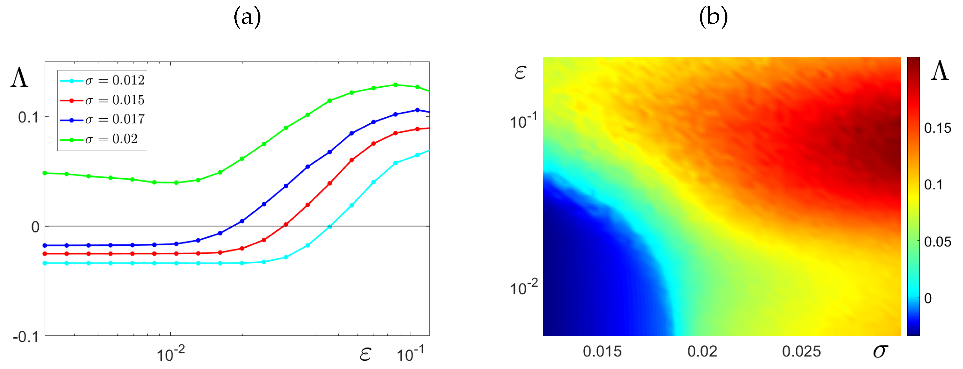
Finally, in Figure 13, we present the largest Lyapunov exponent , which serves as a key indicator of system stability. This exponent provides a quantitative criterion for distinguishing between regular dynamics () and chaotic behavior ().
Figure 13(a) shows as a function of noise intensity for various coupling strengths , while Figure 13(b) illustrates the dependence of on both control parameters, and . From these graphs, one can estimate the threshold noise intensity at which the system transitions from order to chaos. For instance, at , this transition occurs around . It is worth noting that this noise level also corresponds to the onset of stochastic excitation, as previously illustrated in Figure 8(a).
5. Conclusion
In this study, we examined the stochastic disruption of synchronization in a system of two non-identical Rulkov neurons coupled via an electrical synapse. Our analysis uncovered regions of mono-, bi-, and tristability, demonstrating how distinct synchronization regimes arise as a function of coupling strength. Through parametric exploration, we identified conditions under which stochastic perturbations to the coupling parameter induce a transition from lag synchronization to monostable in-phase synchronization.
A central finding of this work is the noise-induced intermittency within the synchronous 3-cycle regime, where increasing noise intensity leads to transient episodes of desynchronization characterized by chaotic bursts. We showed that this behavior is closely linked to the presence of chaotic transient basins, which act as precursors to the disruption of stable synchronization. Moreover, we identified a specific range of noise intensities where this intermittency persists, with its statistical properties—such as laminar phase duration—being highly sensitive to the coupling strength.
Methodologically, the study combines direct numerical simulations with an analytical framework based on confidence ellipses, providing a powerful tool for identifying and predicting the onset of noise-induced excitations. These findings advance our understanding of how stochastic effects influence synchronization in coupled neuronal systems and offer valuable insights into noise-driven dynamics in both biological and artificial neural networks.
Future directions include extending this framework to larger and more complex networks, exploring the role of network topology, and investigating practical implications for neuromorphic engineering and biomedical modeling of brain activity under noisy conditions.
Author Contributions
Conceptualization – I.A.B, L.B.R, and A.N.P.; methodology – L.B.R.; software – I.A.B. and I.N.T.; validation – I.A.B. and L.B.R.; formal analysis – I.A.B.; investigation – L.B.R., I.N.T., and A.N.P.; data curation – I.A.B. and L.B.R.; writing—original draft preparation – I.A.B., L.B.R., and A.N.P.; writing—review and editing – I.A.B., L.B.R., and A.N.P.; visualization – I.A.B. and A.N.P.; supervision – L.B.R.; funding acquisition – I.A.B. and L.B.R. All authors have read and agreed to the published version of the manuscript.
Funding
This work was supported by the Russian Science Foundation (N 24-11-00097).
Data Availability Statement
The original contributions presented in this study are included in the article material. Further inquiries can be directed to the corresponding authors.
Conflicts of Interest
The authors declare no conflicts of interest.
References
- Pikovsky, A.S.; Rosenblum, M.G.; Kurths, J. Synchronization: A Universal Concept in Nonlinear Sciences; Cambridge University Press: Cambridge, 2001. [Google Scholar]
- Boccaletti, S.; Pisarchik, A.N.; del Genio, C.I.; Amann, A. Synchronization: From Coupled Systems to Complex Networks; Cambridge University Press: Cambridge, 2018. [Google Scholar]
- Ghosh, D.; Frasca, M.; Rizzo, A.; Majhi, S.; Rakshit, S.; Alfaro-Bittner, K.; Boccaletti, S. The synchronized dynamics of time-varying networks. Phys. Rep. 2022, 949, 1–63. [Google Scholar] [CrossRef]
- Wu, X.; Wu, X.; Wang, C.Y.; Mao, B.; Lu, J.; Lü, J.; Zhang, Y.C.; Lü, L. Synchronization in multiplex networks. Phys. Rep. 2024, 1060, 1–54. [Google Scholar] [CrossRef]
- Destexhe, A.; Rudolph-Lilith, M. Neuronal Noise; Vol. 8, Springer: New York, 2012. [Google Scholar]
- Kelly, F.; Yudovina, E. Stochastic Networks; Vol. 2, Cambridge University Press: Cambridge, 2014. [Google Scholar]
- Kulkarni, A.; Ranft, J.; Hakim, V. Synchronization, stochasticity, and phase waves in neuronal networks with spatially-structured connectivity. Front. Comput. Neurosci. 2020, 14, 569644. [Google Scholar] [CrossRef] [PubMed]
- Olin-Ammentorp, W.; Beckmann, K.; Schuman, C.D.; Plank, J.S.; Cady, N.C. Stochasticity and robustness in spiking neural networks. Neurocomputing 2021, 419, 23–36. [Google Scholar] [CrossRef]
- Kurrer, C.; Schulten, K. Noise-induced synchronous neural oscillations. Phys. Rev. E 2002, 51, 6213–6218. [Google Scholar] [CrossRef]
- Zhou, H.; Liu, Z.; Li, W. Sampled-data intermittent synchronization of complex-valued complex network with actuator saturations. Nonlin. Dyn. 2022, 107, 1023–1047. [Google Scholar] [CrossRef]
- Pisarchik, A.N.; Hramov, A.E. Stochastic processes in the brain’s neural network and their impact on perception and decision-making. Physics-Uspekhi 2023, 66, 1224–1247. [Google Scholar] [CrossRef]
- Kraut, S.; Feudel, U.; Grebogi, C. Preference of attractors in noisy multistable systems. Phys. Rev. E 1999, 59, 5253–5260. [Google Scholar] [CrossRef]
- Kraut, S.; Feudel, U. Multistability, noise, and attractor hopping: the crucial role of chaotic saddles. Phys. Rev. E 2002, 66, 015207. [Google Scholar] [CrossRef]
- Koronovskii, A.A.; Hramov, A.E.; Grubov, V.V.; Moskalenko, O.I.; Sitnikova, E.; Pavlov, A.N. Coexistence of intermittencies in the neuronal network of the epileptic brain. Phys. Rev. E 2016, 93, 032220. [Google Scholar] [CrossRef]
- Pisarchik, A.N.; Hramov, A.E. Multistability in Physical and Living Systems: Characterization and Applications; Springer: Cham, 2022. [Google Scholar]
- Rulkov, N.F. Regularization of synchronized chaotic bursts. Phys. Rev. Lett. 2001, 86, 183–186. [Google Scholar] [CrossRef] [PubMed]
- Ge, P.; Cao, H. Chaos in the Rulkov neuron model based on Marotto’s theorem. Int. J. Bifurcat. Chaos 2021, 31, 2150233. [Google Scholar] [CrossRef]
- Wang, Y.; Zhang, X.; Liang, S. New phenomena in Rulkov map based on Poincaré cross section. Nonlin. Dyn. 2023, 111, 19447–19458. [Google Scholar] [CrossRef]
- Bashkirtseva, I.; Ryashko, L. Transformations of spike and burst oscillations in the stochastic Rulkov model. Chaos Soliton. Fract. 2023, 170, 113414. [Google Scholar] [CrossRef]
- Li, G.; Duan, J.; Yue, Z.; Li, Z.; Li, D. Dynamical analysis of the Rulkov model with quasiperiodic forcing. Chaos Soliton. Fract. 2024, 189, 115605. [Google Scholar] [CrossRef]
- Bashkirtseva, I.A.; Pisarchik, A.N.; Ryashko, L.B. Coexisting attractors and multistate noise-induced intermittency in a cycle ring of Rulkov neurons. Mathematics 2023, 11, 597. [Google Scholar] [CrossRef]
- Marghoti, G.; Ferrari, F.A.S.; Viana, R.L.; Lopes, S.R.; Prado, T.d.L. Coupling dependence on chaos synchronization process in a network of Rulkov neurons. Int. J. Bifurcat. Chaos 2023, 33, 2350132. [Google Scholar] [CrossRef]
- Bashkirtseva, I.A.; Pisarchik, A.N.; Ryashko, L.B. Multistability and stochastic dynamics of Rulkov neurons coupled via a chemical synapse. Commun. Nonlinear Sci. Numer. Simul. 2023, 125, 107383. [Google Scholar] [CrossRef]
- Ge, P.; Cheng, L.; Cao, H. Complete synchronization of three-layer Rulkov neuron network coupled by electrical and chemical synapses. Chaos 2024, 34. [Google Scholar] [CrossRef]
- Le, B.B. Asymmetric coupling of nonchaotic Rulkov neurons: Fractal attractors, quasimultistability, and final state sensitivity. Phys. Rev. E 2025, 111, 034201. [Google Scholar] [CrossRef]
- Bashkirtseva, I.; Ryashko, L. Stochastic sensitivity analysis of noise-induced phenomena in discrete systems. In Recent Trends in Chaotic, Nonlinear and Complex Dynamics; World Scientific Series on Nonlinear Science Series B, 2021; chapter 8, pp. 173–192.
- Bashkirtseva, I.; Nasyrova, V.; Ryashko, L. Analysis of noise effects in a map-based neuron model with Canard-type quasiperiodic oscillations. Commun. Nonlinear Sci. Numer. Simulat. 2018, 63, 261–270. [Google Scholar] [CrossRef]
- Garain, K.; Sarathi Mandal, P. Stochastic sensitivity analysis and early warning signals of critical transitions in a tri-stable prey-predator system with noise. Chaos 2022, 32, 033115. [Google Scholar] [CrossRef] [PubMed]
- Stone, E.; Holmes, P. Noise-induced intermittency in a model of turbulent boundary layer. Physica D 1989, 37, 20–32. [Google Scholar] [CrossRef]
- Platt, N.; Hammel, S.M.; Heagy, J.F. Effects of additive noise on on-off intermittency. Phys. Rev. Lett. 1994, 72, 3498. [Google Scholar] [CrossRef]
- Heagy, J.F.; Platt, N.; Hammel, S.M. Characterization of on-off intermittency. Phys. Rev. E 1994, 48, 1140. [Google Scholar] [CrossRef]
- Fujisaka, H.; Ouchi, K.; Ohara, H. On-off convection: Noise-induced intermittency near the convection threshold. Phys. Rev. E 2001, 64, 036201. [Google Scholar] [CrossRef]
- Moskalenko, O.; Koronovskii, A.A.; Zhuravlev, M.O.; Hramov, A.E. Characteristics of noise-induced intermittency. Chaos Soliton. Fract. 2018, 117, 269–275. [Google Scholar] [CrossRef]
Figure 1.
Bifurcation diagram (blue) and Lyapunov exponent (red) of the isolated Rulkov system. The crisis bifurcation occurs at .
Figure 1.
Bifurcation diagram (blue) and Lyapunov exponent (red) of the isolated Rulkov system. The crisis bifurcation occurs at .
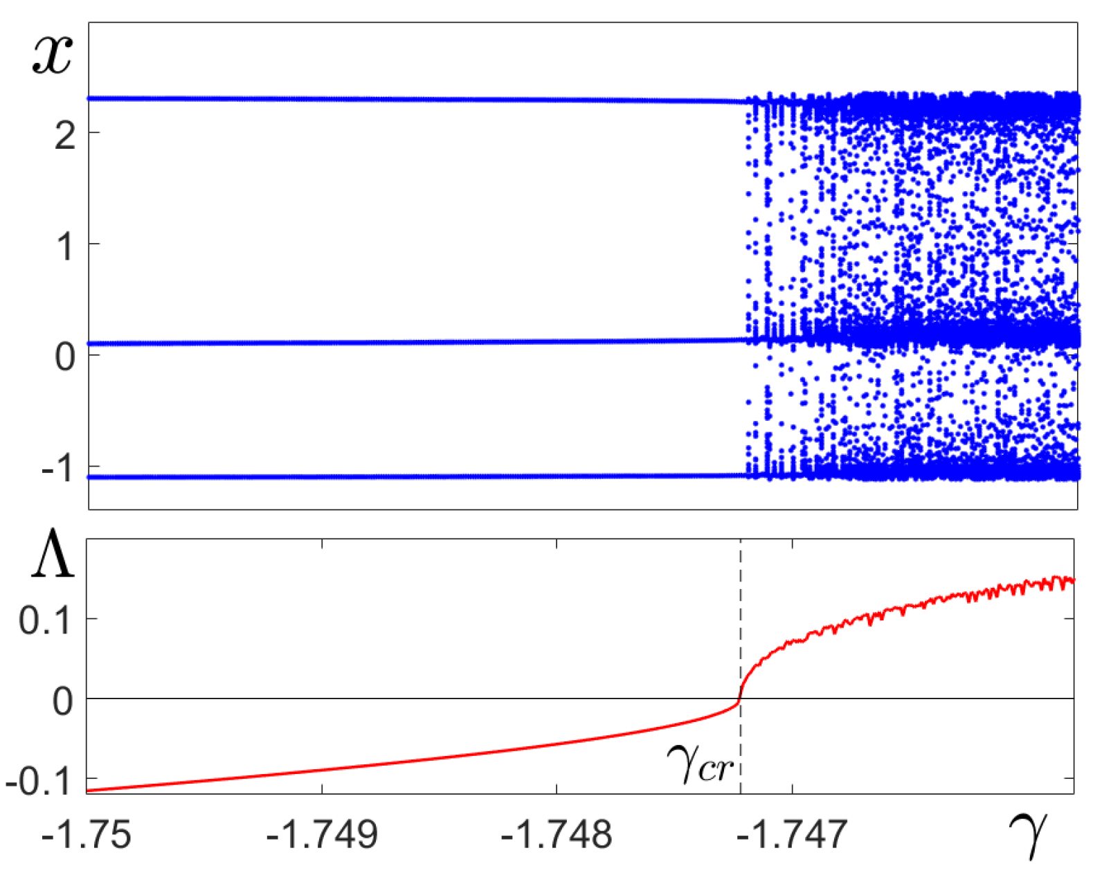
Figure 2.
Bifurcation diagram of system (1) with and . The coexisting 3-cycles , , and and shown in blue, green, and orange, respectively.
Figure 2.
Bifurcation diagram of system (1) with and . The coexisting 3-cycles , , and and shown in blue, green, and orange, respectively.
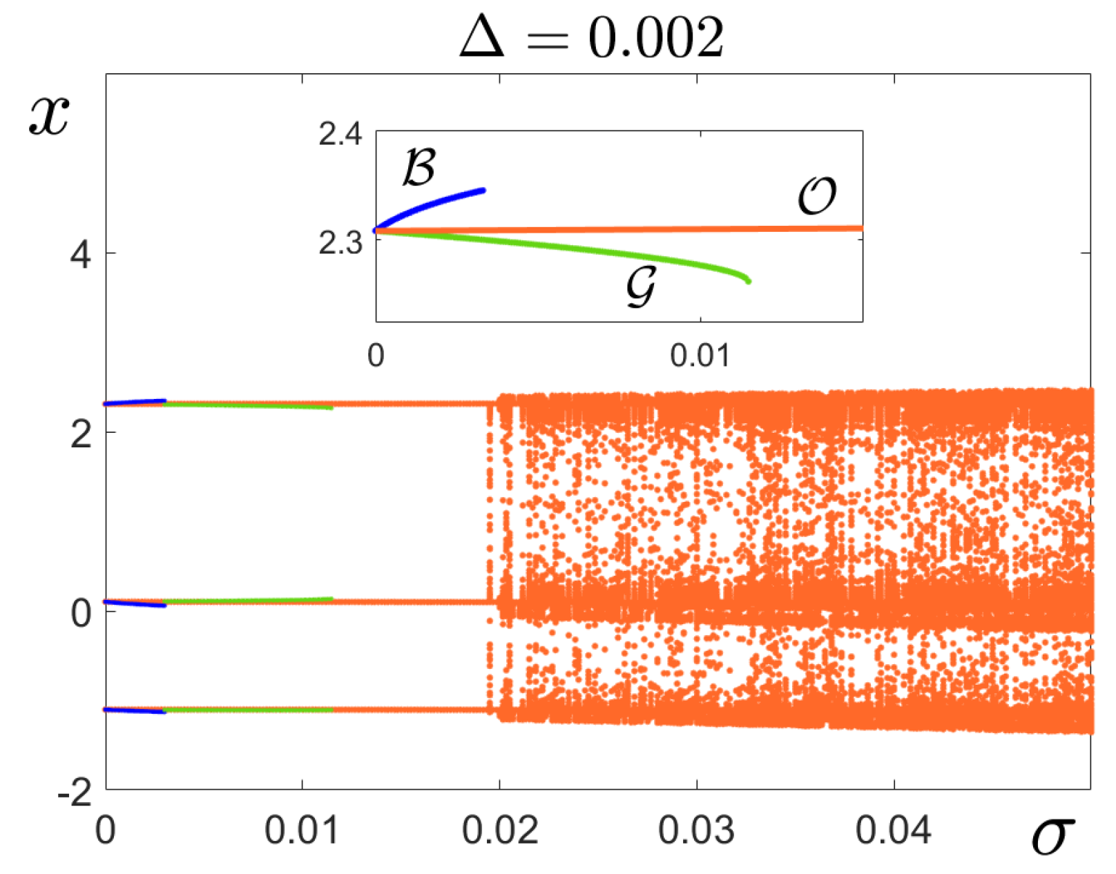
Figure 3.
Attractors and their basins of attraction of system (1) with and at coupling strengths: (a) , tristability; (b) , bistability; (c) , monostability; and (d) , chaotic attractor.
Figure 3.
Attractors and their basins of attraction of system (1) with and at coupling strengths: (a) , tristability; (b) , bistability; (c) , monostability; and (d) , chaotic attractor.
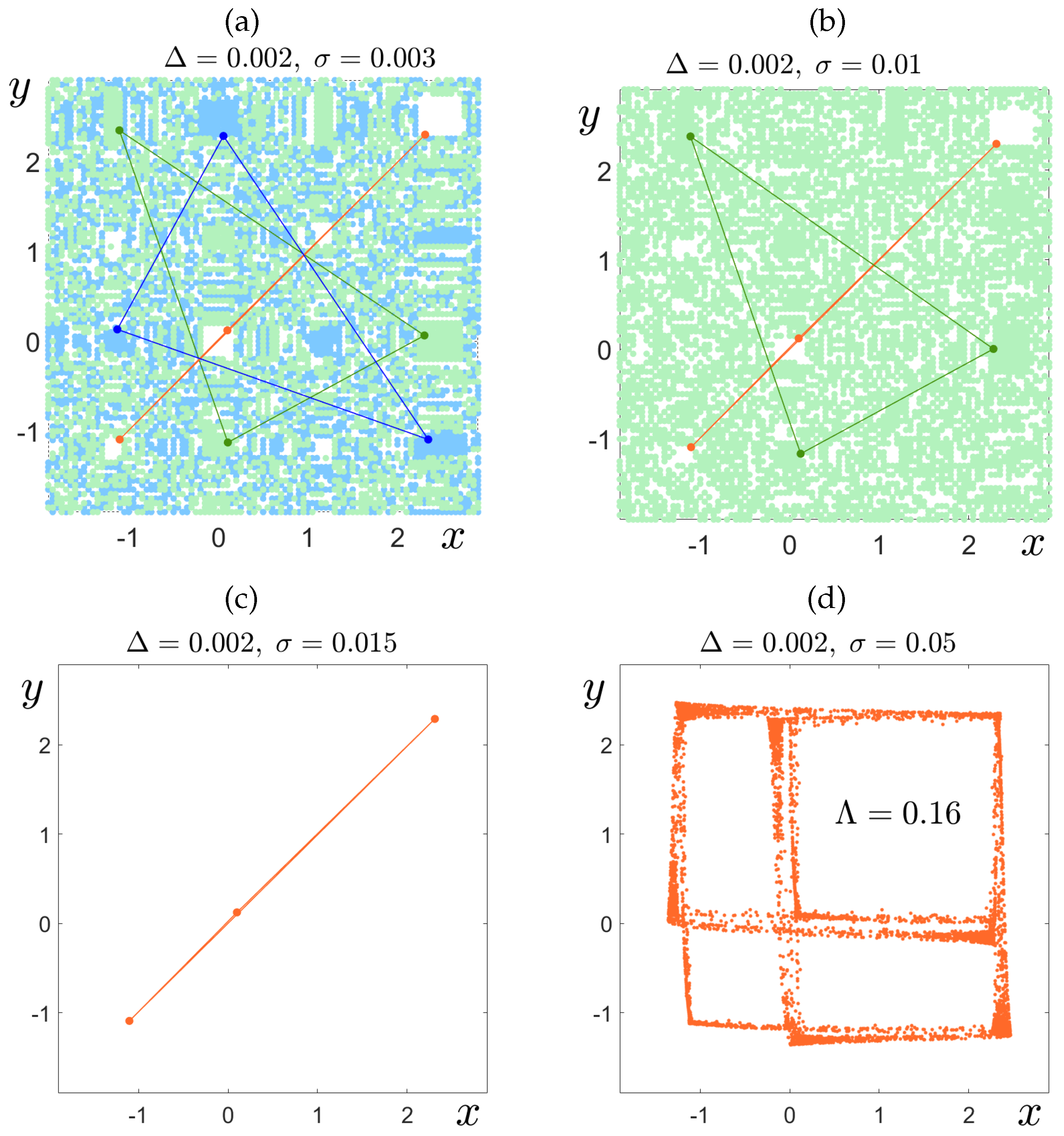
Figure 4.
Time series of the () coordinate in system (2) with , starting from cycles (orange), (green), and cycle (blue) under different noise intensities: (a) , (b) , (c) . (d) Random states of system (2) with .
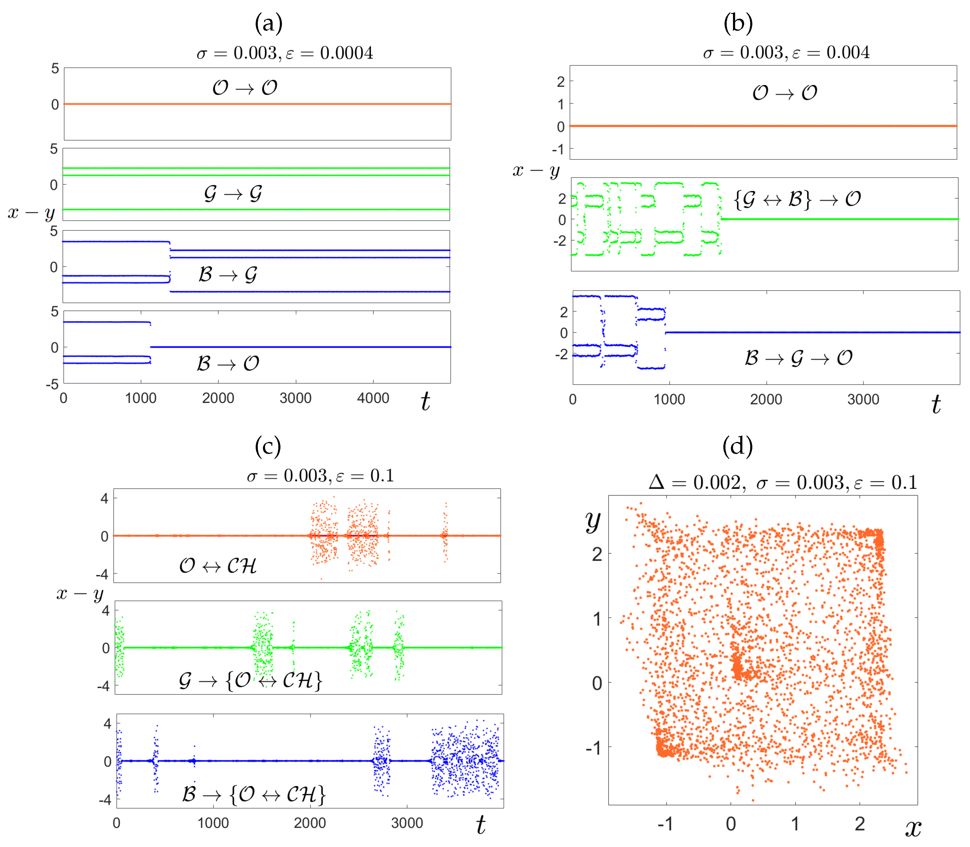
Figure 5.
Stochastic transitions in the () solutions of system (2) with , and as a function of noise intensity , starting from (a) cycle (blue), (b) cycle (green), and (c) orange cycle (orange).
Figure 5.
Stochastic transitions in the () solutions of system (2) with , and as a function of noise intensity , starting from (a) cycle (blue), (b) cycle (green), and (c) orange cycle (orange).
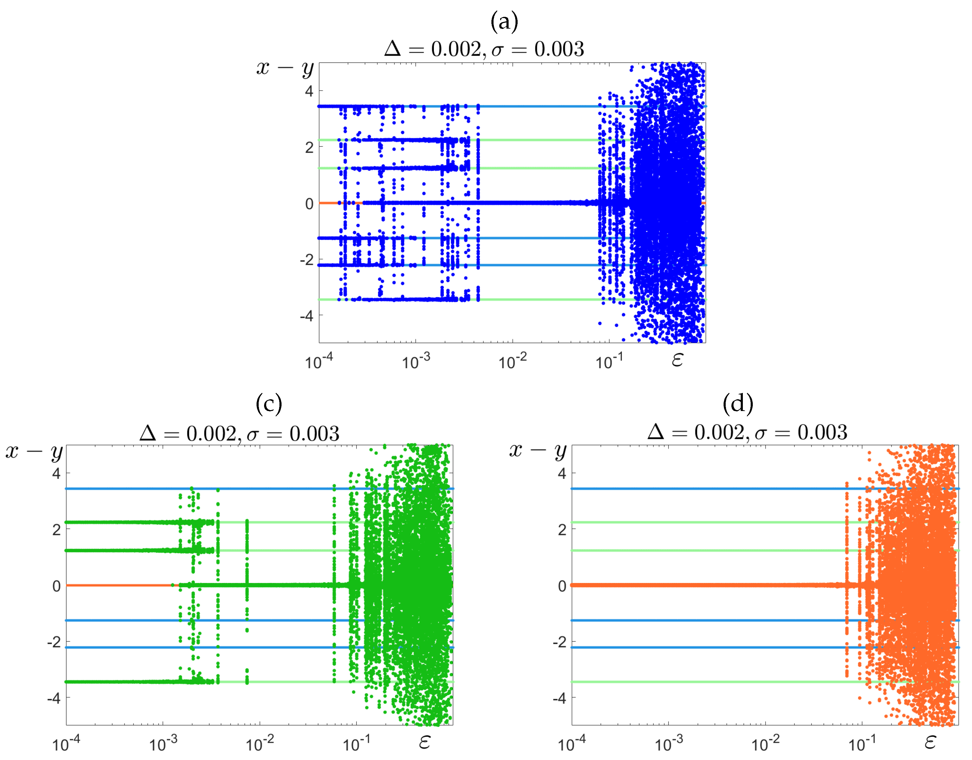
Figure 6.
Illustration of the confidence domain method in the stochastic system (2) with , , and . Enlarged fragments of the phase plane of the deterministic system (1) show the basins of cycle (light blue), cycle (light green), and cycle (white), along with confidence ellipses: (a) around the state of for (blue) and (red); (b) around the state of for ; (c) around the state of for ; and (d) around the state of for (blue) and (red).
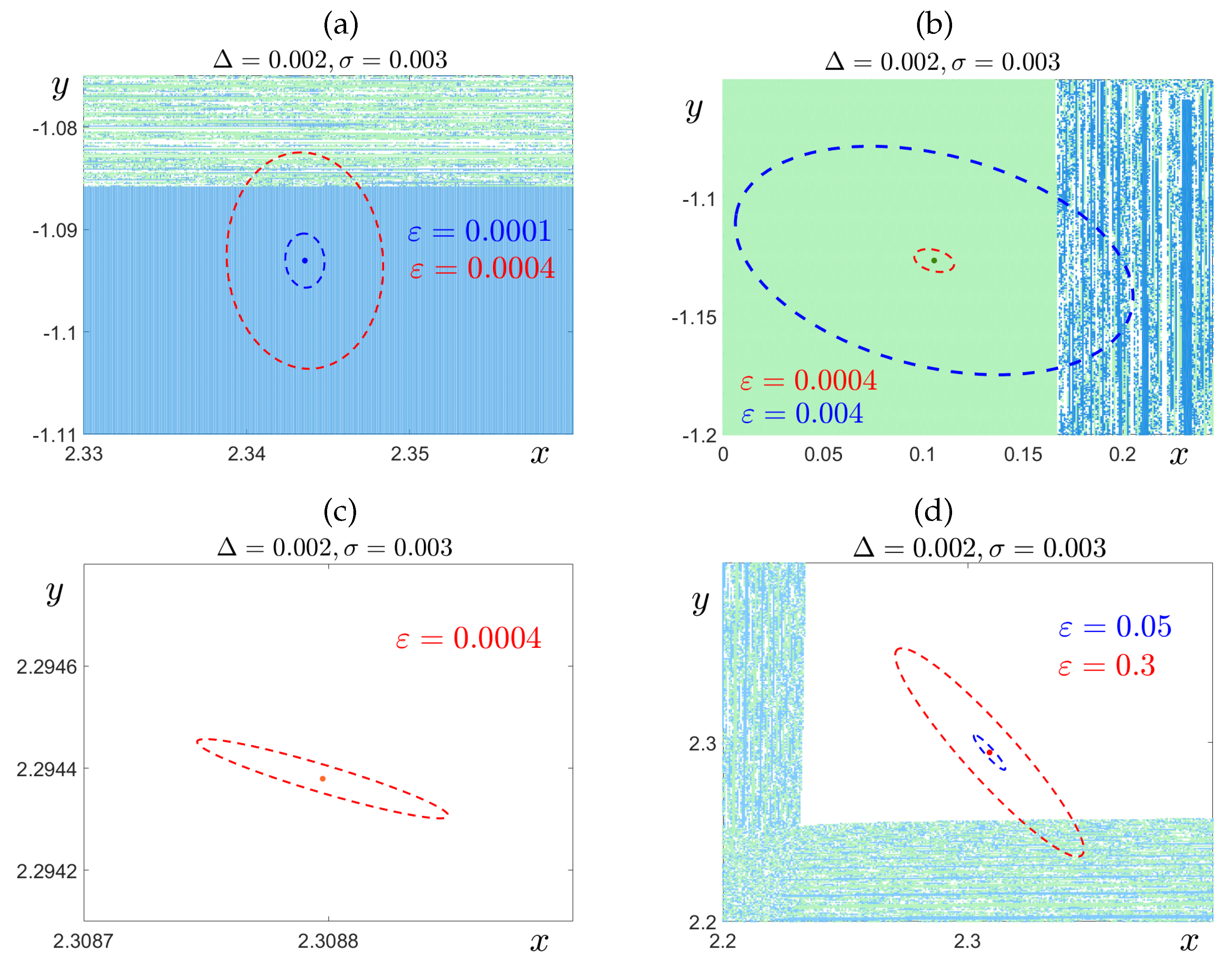
Figure 7.
Stochastic transitions in system (2) with , , and . (a) Random states of solutions originating from cycle (green) under varying noise intensity . (b) Random states of solutions originating from cycle (orange). (c) Enlarged fragment of the phase plane showing confidence ellipses around a state of cycle for (blue) and (red). (d) Enlarged fragment with confidence ellipses around the state of cycle for (blue) and (red).
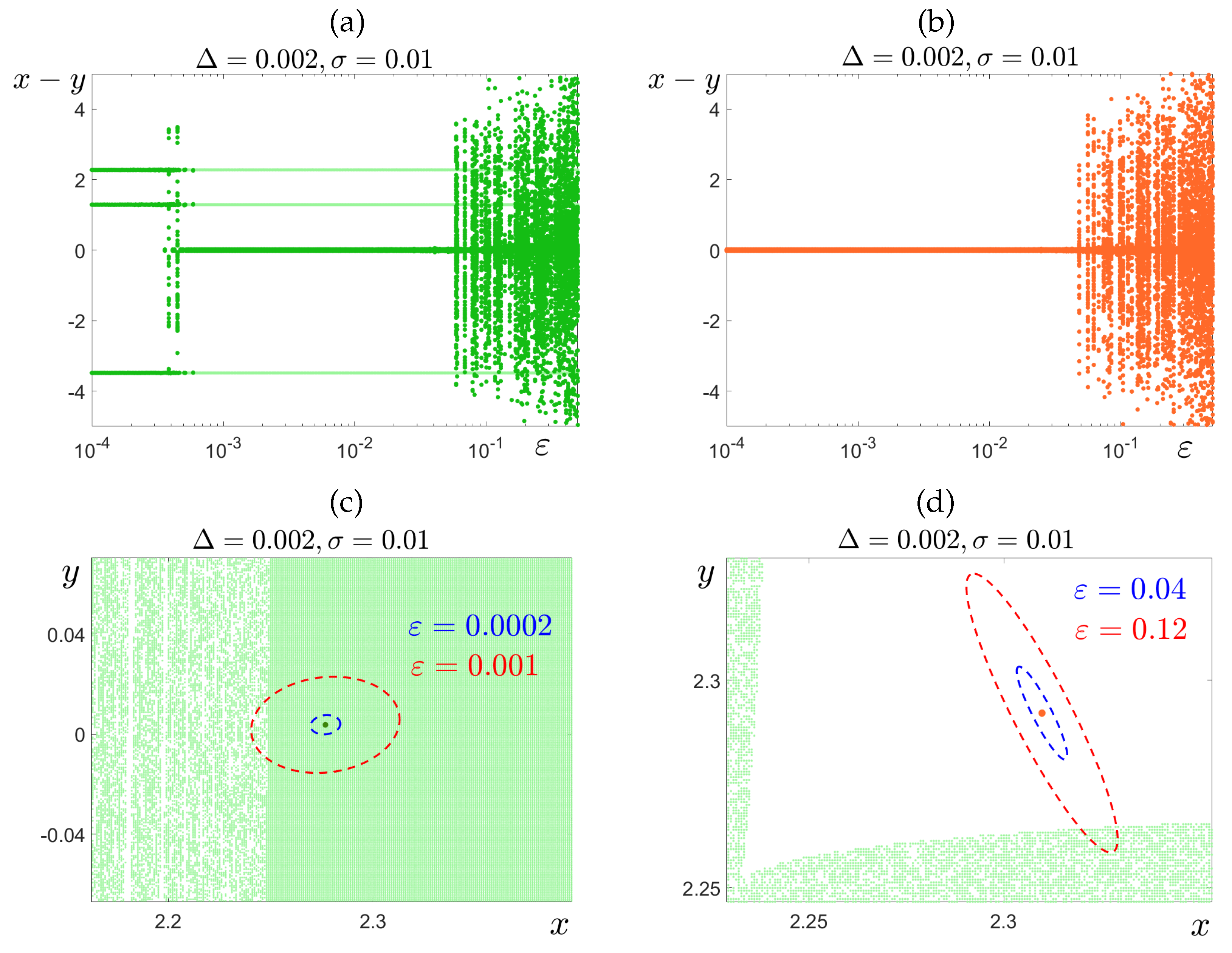
Figure 8.
Noise-induced excitation of system (2) with parameters , , and : (a) Random states for solutions initiated at cycle (orange) versus noise intensity ; (b) Phase space representation of random states for (blue), showing localization near cycle , and for (orange), illustrating widespread dispersion due to noise-induced excitation.
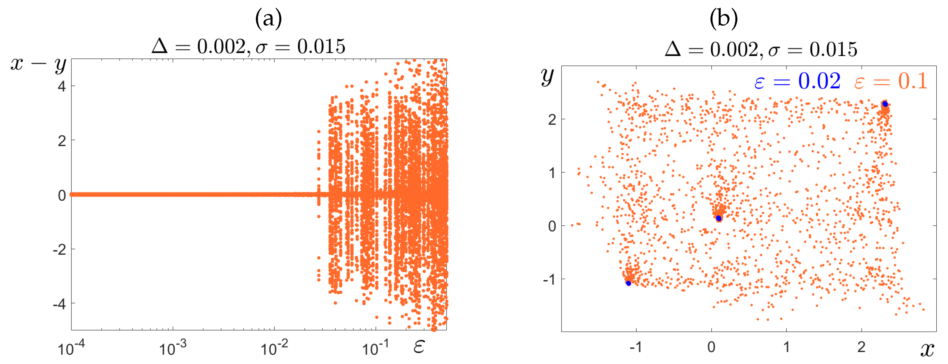
Figure 9.
Transient dynamics of deterministic system (1) with , , and . (a) Basin of short transients (white region), where trajectories reach cycle within 200 iterations with an accuracy of 0.001. (b) Zoomed-in fragment showing confidence ellipses for (blue) and (red), along with reference points and . (c) Time series of (blue) (upper panel) and synchronization indicator z (red) (lower panel) for a trajectory starting at point . (d) Same as in (c), but for a trajectory starting at point . (e) Representative examples of transient dynamics for various initial conditions .
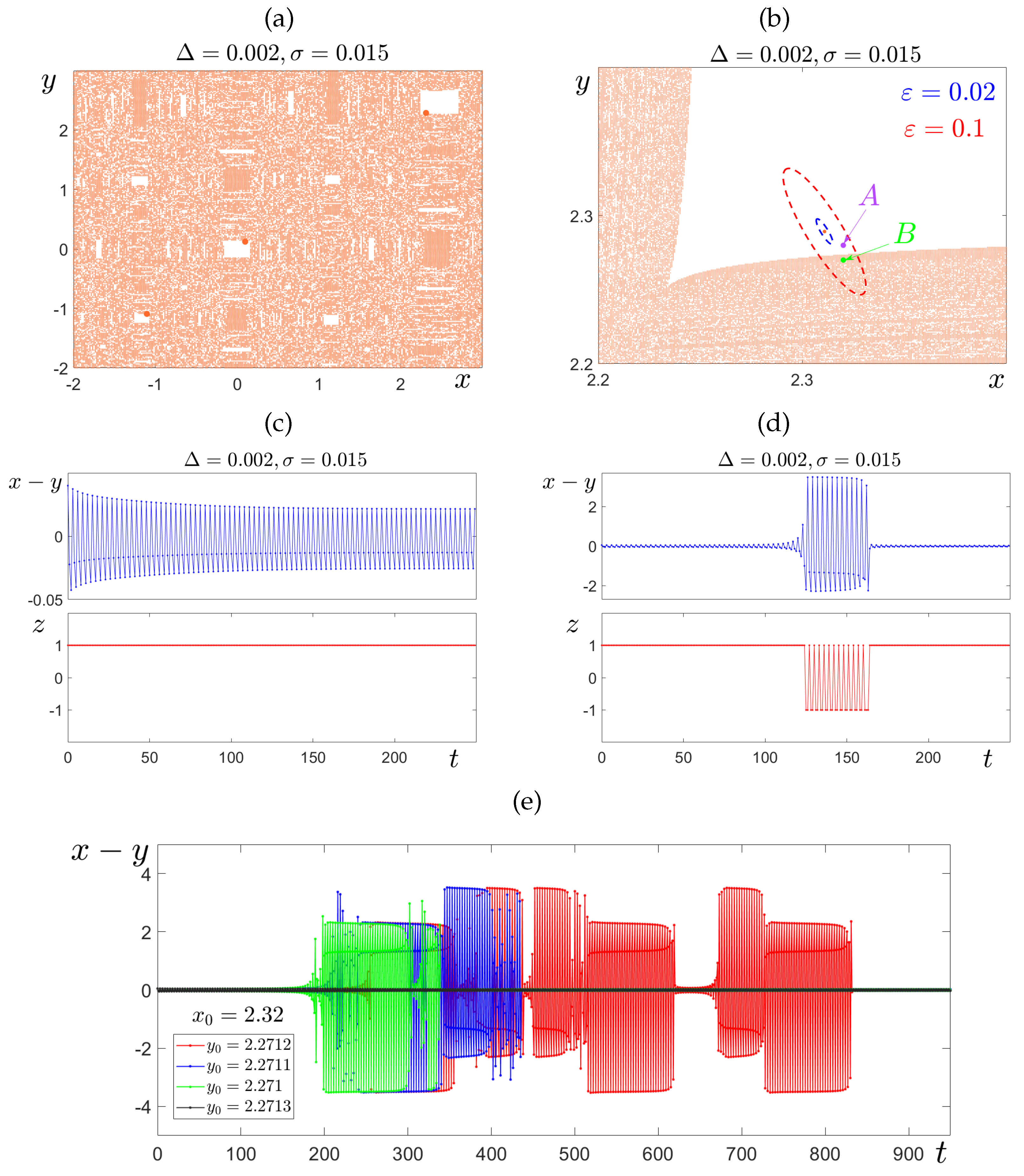
Figure 10.
Color map showing the convergence rate of solutions of the deterministic system (1) to the 3-cycle . The color indicates the number of iterations required to achieve a convergence accuracy of 0.001. The red dashed line represents the confidence ellipse for the corresponding stochastic system (2) with noise intensity .
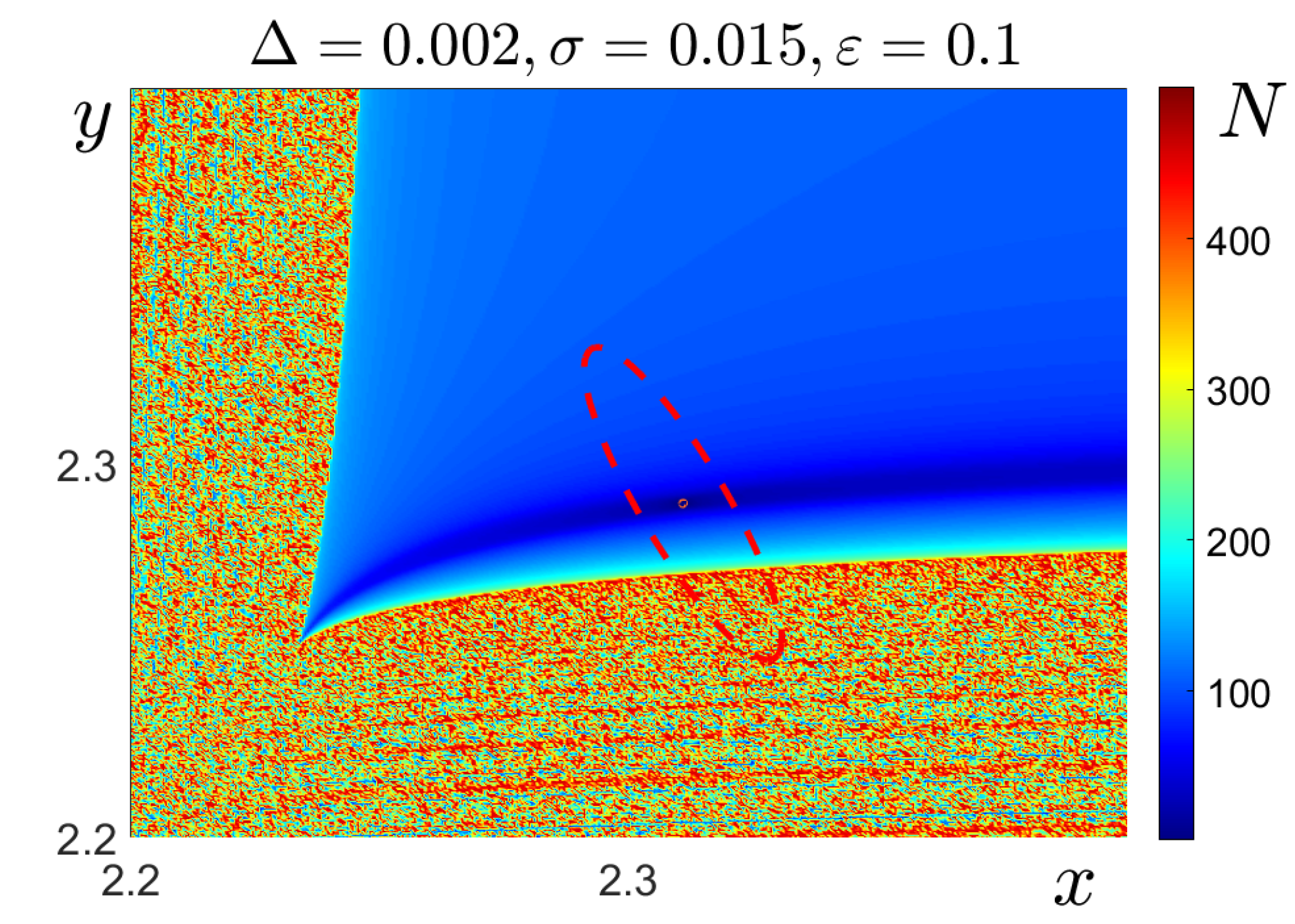
Figure 11.
Time series of the x-coordinate (green) and the synchronization indicator z (blue) for solutions of the stochastic system (2), initialized at the deterministic 3-cycle for noise intensities (a) and (b) .
Figure 11.
Time series of the x-coordinate (green) and the synchronization indicator z (blue) for solutions of the stochastic system (2), initialized at the deterministic 3-cycle for noise intensities (a) and (b) .
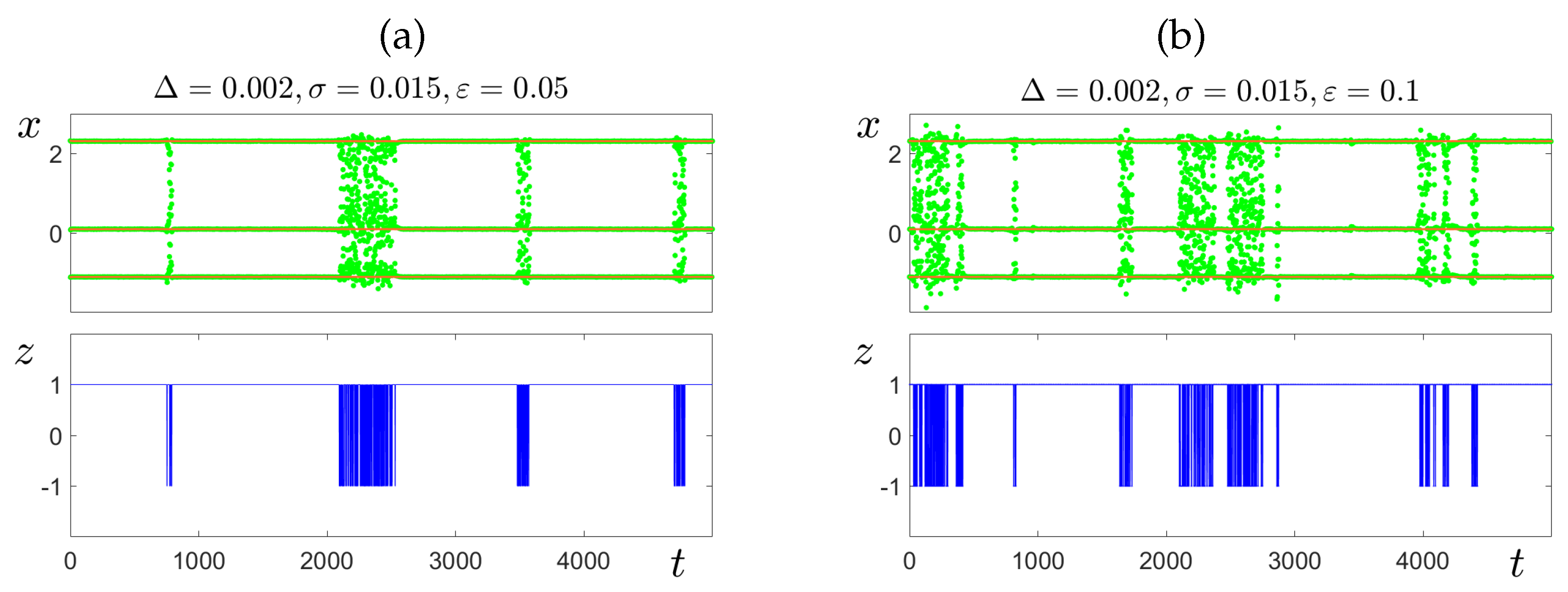
Figure 12.
Characteristics of noise-induced intermittency in the stochastic system (2) with and . (a) Mean duration of laminar phases corresponding to co-directed behavior () as a function of noise intensity for various coupling strengths . (b) Probability of observing co-directed behavior as a function of noise intensity for different values. (c) Mean duration of synchronization intervals (with ) plotted against deviation d of from crisis bifurcation point , where .
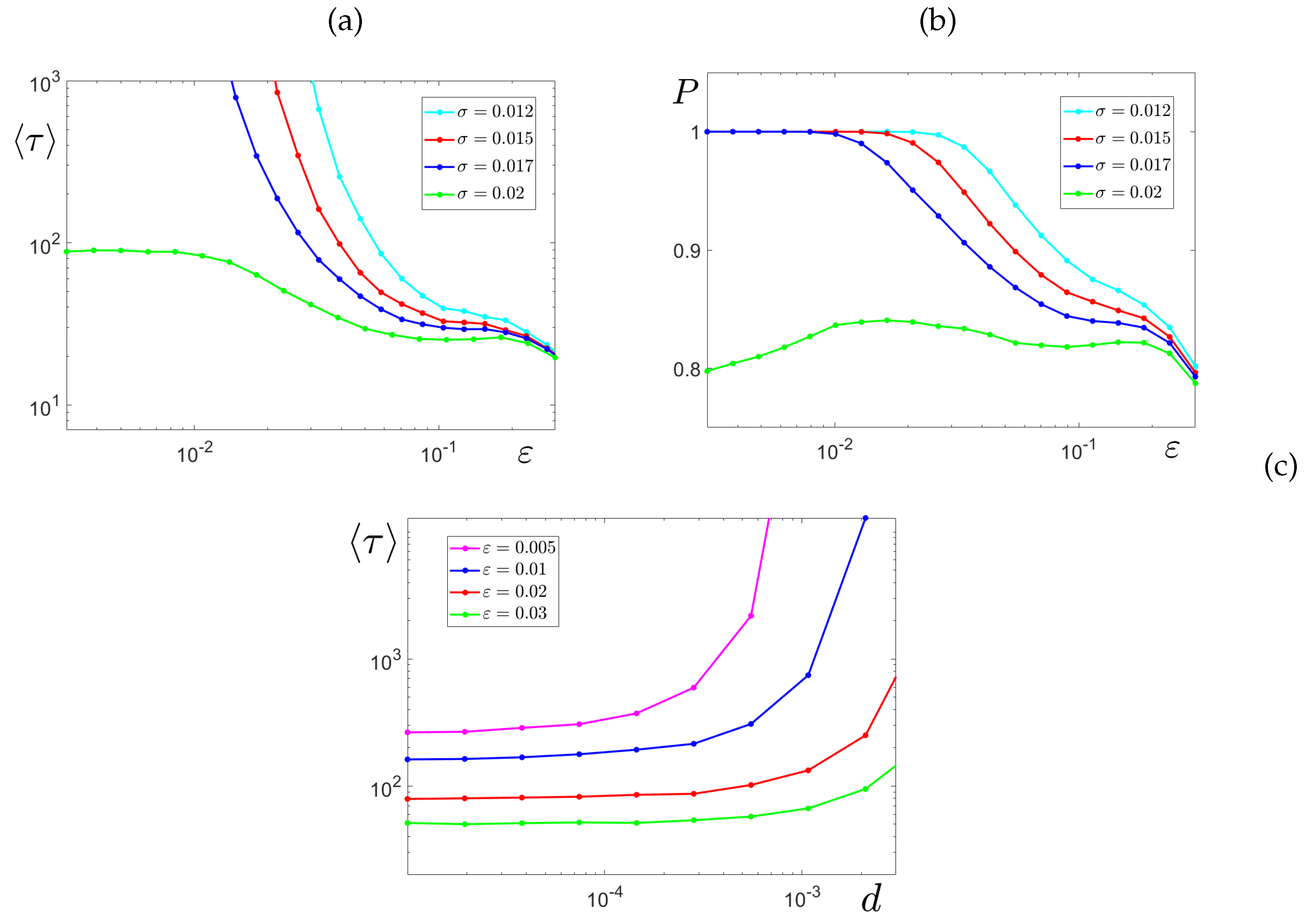
Figure 13.
Largest Lyapunov exponent of the stochastic system (2) with and . (a) as a function of noise intensity for different values of the coupling strength . (b) Two-parameter diagram of in the -plane, illustrating the transition from regular to chaotic dynamics.
Figure 13.
Largest Lyapunov exponent of the stochastic system (2) with and . (a) as a function of noise intensity for different values of the coupling strength . (b) Two-parameter diagram of in the -plane, illustrating the transition from regular to chaotic dynamics.
Disclaimer/Publisher’s Note: The statements, opinions and data contained in all publications are solely those of the individual author(s) and contributor(s) and not of MDPI and/or the editor(s). MDPI and/or the editor(s) disclaim responsibility for any injury to people or property resulting from any ideas, methods, instructions or products referred to in the content. |
© 2025 by the authors. Licensee MDPI, Basel, Switzerland. This article is an open access article distributed under the terms and conditions of the Creative Commons Attribution (CC BY) license (http://creativecommons.org/licenses/by/4.0/).
Copyright: This open access article is published under a Creative Commons CC BY 4.0 license, which permit the free download, distribution, and reuse, provided that the author and preprint are cited in any reuse.


