
Submitted:
18 October 2023
Posted:
19 October 2023
You are already at the latest version
Abstract
An algorithm is proposed for discriminating the fatigue state of air traffic controllers based on ap-plying multispeech feature fusion using an FSVM to voice data, and for extracting eye-fatigue-state discrimination features based on PERCLOS eye data. For the speech algorithm and an eye-fatigue index, a new controller fatigue-state evaluation index based on the entropy weight method is proposed based on decision-level fusion of fatigue discrimination results for speech and the eyes. Experimental results show that the fatigue-state recognition accuracy rate was 84.81% for the fatigue state evaluation index, which was 3.36% and 1.86% higher than those for speech and eye assessments, respectively. The comprehensive fatigue evaluation index provides important reference values for controller scheduling and mental-state evaluations.
Keywords:
fatigue recognition
; Air traffic controller
; Feature fusion
; Multi-mode
; scheduling
1. Introduction
The rapid increase in flight volume has increased the workload of air traffic controllers, which may lead to unsafe incidents in civil aviation transportation and endanger the safe operation of civil aviation. [1] Therefore, research into fatigue detection of controllers has become a crucial topic in the field of civil aviation. How to effectively detect the fatigue state of controllers and objectively manage their fatigue based on the detection results have become a major research focus of civil aviation scholars.
In recent years there have been many research studies into objective methods for fatigue detection. Wu et al. [2] found through experiments that time-domain, frequency-domain, and nonlinear heart-rate features of the electrocardiogram (ECG) change with fatigue, and hence they can be used as characteristic indicators for fatigue detection. Zhao et al. [3] used simulated-fatigue driving experiments to quantify changes in the electroencephalogram (EEG) and ECG with the degree of fatigue, and proposed a method for detecting fatigue using the EEG and ECG. However, the invasiveness of such contact-based fatigue-detection methods can affect the work of controllers. Therefore, this study investigated a noncontact fatigue monitoring method. At the same time, in order to improve the recognition accuracy of controller fatigue speech, this paper fuses speech features with facial features to improve the recognition accuracy.
Traditional speech signal processing is based on linear theory. Based on their short-term resonance characteristics, speech signals can be simulated as time series composed of an excitation source and a filter to construct a classic speech signal excitation-source–filter model [4]. These signals can be described using various parameters in the model in order for them to be processed and analyzed.
When the human body is in a state of fatigue, speech signals will exhibit a decrease in pitch frequency and changes in the position and bandwidth of the spectral resonance peak. These changes are due to relaxation of the vocal cord muscles [5]. At the same time, the slowing of brain vitality caused by fatigue can also affect the speech speed and clarity, causing changes in parameters such as time–frequency power spectral coefficients and speechless modes of speech signals [6]. Therefore, the speech signal can be used to characterize the impact of fatigue on the human body. Li [7] conducted a speech-fatigue test on members of an American bombing crew, and found that the pitch and bandwidth of their speech signals showed significant changes after a long flight. Krajewski [8] extracted 8500 features from frame-level speech samples, and after feature dimensionality reduction and feature recognition, obtained feature vectors for characterizing fatigue with an accuracy of 76.5% in experiments.
Speech-signal research has led to scholars concluding that the generation process of speech signals is a nonlinear process; that is, it is neither a deterministic linear sequence nor a random sequence, but rather a nonlinear sequence with chaotic components. Therefore, traditional linear filter models are too simplistic in characterizing speech signals and cannot fully present the information contained in speech signals [9]. A nonlinear dynamic model of a speech signal is generally constructed using a delay-phase diagram that is obtained by reconstructing the time series of a one-dimensional speech signal in phase space [10]. Previous studies have shown that the fatigue state of the human body influences the phase-space track of speech, especially the degree of chaos in its phase space [11].
At present, fatigue in air traffic controllers is mostly detected using a single index, or only using the method of feature fusion. In contrast, this study collected fatigue characteristics from two different sensors to reflect human fatigue from different aspects. In order to supplement the speech fatigue features and improve the accuracy of fatigue recognition, we choose to use facial information to expand the dimensions of fatigue features. Many scholars have considered information about the eye in research into fatigue detection. Wierwille [12] analyzed the relationship between a driver’s eye closure time and the collision probability in experiments on driving fatigue, and found that eye closure time can be used to characterize fatigue. The US Transportation Administration also conducted experiments investigating nine parameters including blink frequency, closure time, and eyelid closure, and demonstrated that these characteristics can also be used to characterize the degree of fatigue. Jo et al. [13] proposed an algorithm for determining the eye position of drivers based on blob features [14]. They then applied principal-components analysis [15] and linear discriminant analysis to extract ocular features, and finally judged the fatigue state of a driver using a support vector machine (SVM) classifier. The commonly used algorithms for fusing each attribute feature layer are machine-learning algorithms, mainly including the Gaussian mixture model, SVM, and artificial neural networks to obtain the decision results of the feature layer. In decision-level fusion, methods such as linear combination, the entropy weight method, and a Bayesian network are used to obtain the final results for fatigue detection.
In our previous work, we only collected voice data, and there is still an improvement range for fatigue state discrimination of voice data, so the experiment in this paper not only contains voice data, but also collects facial data as a supplement to speech data. In this paper, the classifier is trained based on the previously collected speech data. In order to verify the effectiveness of the fatigue state discrimination method of the decision layer, this paper complements the speech data and face experimental data, and uses the latest collected data as the test set for fatigue state discrimination.
This paper presents a decision level fusion method based on voice data and eye data to discriminate fatigue state of controllers. In the process of speech fatigue feature extraction, we carry out feature level fusion on the speech fatigue features extracted by different methods. For the speech fatigue features after fusion, we use two different classifiers, FSVM and SVM, respectively, to obtain two types of results based on speech data. We used PERCLOS and Maximum Continuous Eye Closure Duration (MECD)as complements to the speech features, and used threshold method to identify the state of eye fatigue according to the different states of controllers. In this way, we realized two kinds of controller fatigue state discrimination based on voice features and facial features. In order to solve the conflict between the two kinds of discrimination results, we use entropy weight method to fuse the two kinds of discrimination results at decision level to achieve a more accurate discrimination of fatigue state.
This paper is structured as follows: In section 2, we introduced the multi-level information fusion model of this paper, including the model's feature extraction from data sources, feature fusion, fusion feature recognition, and the decision layer fusion process based on two types of recognition results. In section 3, we introduced the controller fatigue feature extraction recognition experiment carried out in this paper, including the collection process of fatigue data and the processing results according to the model of this paper. The last part is our summary of this paper. Section 4 draws our conclusions, demonstrating that the accuracy of our multi-level information fusion model is enhanced when processed using the FSVM classifier.
2. Methods
In the field of speech processing recognition, there are currently various speech features. We can divide them into three categories: spectral features, statistical features, and nonlinear features. We choose one from each category so that our data fusion can depict speech from three different perspectives. Here we extract the Mel frequency cepstral coefficient (MFCC), short-time-average zero-crossing rate, and maximum Lyapunov index. Based on the percentage of eyelid closure over time (PERCLOS) as eye features, feature fusion was applied to the features of the two types of data sources, and an evaluation index system was established.
The structure of the fatigue evaluation index is shown in Figure 1.
2.1. Speech feature classification algorithm based on the FSVM
In fatigue detection, because the fuzzy samples in the feature space often lead to reduction of the classification interval and affect the classification performance of the classifier [16]. In practical applications, training samples are often affected by some noise. This noise may have adverse effects on the decision boundary of SVM, leading to a decrease in accuracy. To solve this problem, this paper introduces the idea of a fuzzy system and combines it with an FSVM algorithm.
The membership function is first introduced. The algorithm principle of the FVSM is to add a membership function to original sample set so as to change the sample set to . Membership function refers to the probability that the th sample belongs to the category; this is referred to as the reliability, where , and a larger indicates a higher reliability. After introducing the membership function, the SVM formula can be expressed as
Original relaxation variable is replaced by since the original error description of the sample does not meet the conditions for the relaxation variable presented in the form of the weighted error term of . Reducing the membership degree of sample weakens the influence of error term on the objective function. Therefore, when locating the optimal segmentation surface, can be regarded as a secondary (or even negligible) sample feature, which can exert a strong inhibitory effect on isolated samples in the middle zone, and yield a relatively good optimization effect on the establishment of the optimal classification surface. The quadratic programming form of formula (1) is dually transformed to
In this formula, the constraint condition is changed from to , and the weight coefficient is added to penalty coefficient . For samples with different membership degrees, the added penalty coefficients are also different: indicates the ordinary SVM, while when sample becomes too small, and its contribution to the optimal classification plane will also become smaller.
In optimal solution , the support vector is the nonzero solution of . After introducing the membership function, is divided into two parts: (1) the effective support vector distributed on the hyperplane; that is, the sample corresponding to , which meets the constraint condition; and (2) the isolated sample that needs to be discarded according to the rule; that is, the sample corresponding to . Therefore, the classification ability of each SVM is tested by the membership function, and finally the decision model of FSVM is obtained through training as follows:
where
The sample membership function has a large impact on the classification effect of FSVM, and so selecting an appropriate sample membership function is an important step in the design of the FSVM. The commonly used membership functions include the linear membership function, S-type membership function, type membership function [17].
However, the traditional membership function (see Figure 2.2) usually only considers the distance between the sample and the center point. Therefore, when there are isolated samples or noise points close to the center point, they will be incorrectly assigned a higher membership.
As shown in Figure 2a, in the triangle samples of the positive class, distance between the isolated sample and the sample center is basically the same as distance between the support sample and the sample center, and so the two samples will be given the same membership value, which will adversely affect the determination of the optimal classification plane.
In order to avoid the above situation, a membership function of the normal plane is proposed, which involves connecting the center points of positive and negative samples to determine the normal plane, and synchronously determining the hyperplane of the sample attribute. In this approach the sample membership is no longer determined by the distance between the sample and the center point, but by the distance from the sample to the attribute hyperplane. As shown in Figure 2b, the distance between the isolated sample and the sample center becomes , and the distance between the supporting sample and the sample center becomes , which is better at eliminating the influence of isolated samples.
In the specific calculation, first set the central point of positive and negative samples as and , respectively, and and as the number of positive and negative samples, and calculate their center coordinates according to the mean value:
is the vector connecting the centers of the two samples, and normal vector is obtained by transposing . Then the hyperplane to which the two samples belong is
Then the distance from any sample to its category hyperplane is
If the maximum distance between positive samples and the hyperplane is set to , and the maximum distance between negative samples and the hyperplane is set to , then the membership of various inputs is
where takes a small positive value to satisfy .
In the case of nonlinear classification, kernel function is also used to map the sample space to the high-dimensional space. According to mapping relationship , the center points of the positive and negative samples become
The distances from the input sample to the hyperplane can then be expressed as
This formula can be calculated using inner product function in the original space rather than . Then, the distance of positive sample from the positive hyperplane is
Similarly, the distance of negative sample from the negative hyperplane is
Through formula (10) and formula (11), we can use formula (7) to obtain the membership degree in the case of nonlinearity.
2.2. Eye-fatigue feature extraction algorithm based on PERCLOS
This section describes eye feature extraction. PERCLOS refers to the proportion of time that the eye is closed, and is widely used as an effective evaluation parameter in the field of fatigue discrimination. P80 in PERCLOS, which corresponds to the pupil being covered by more than 80% of the eyelid, was the best parameter for fatigue detection, and so we selected this as the judgment standard for eye fatigue[18].
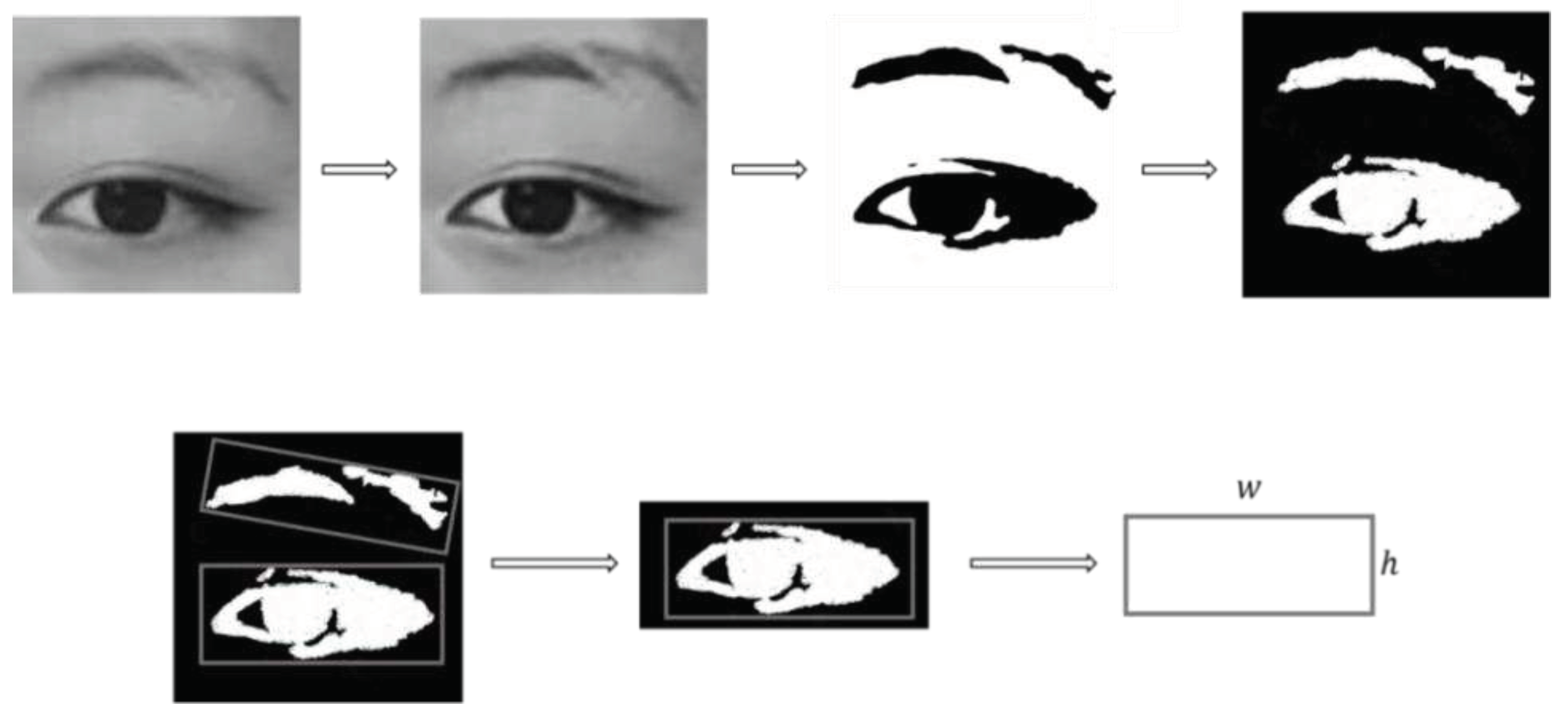
Before extracting PERCLOS, we first need to identify the closed state of the eyes. This is addressed here by analyzing the aspect ratio of the eyes. Figure 3 shows images of a human eye in different states. When the eye is fully closed, the eye height is 0 and aspect ratio is the smallest. Conversely, is largest when the eye is fully open.
We calculate the PERCLOS value by applying the following steps:
1. Histogram equalization
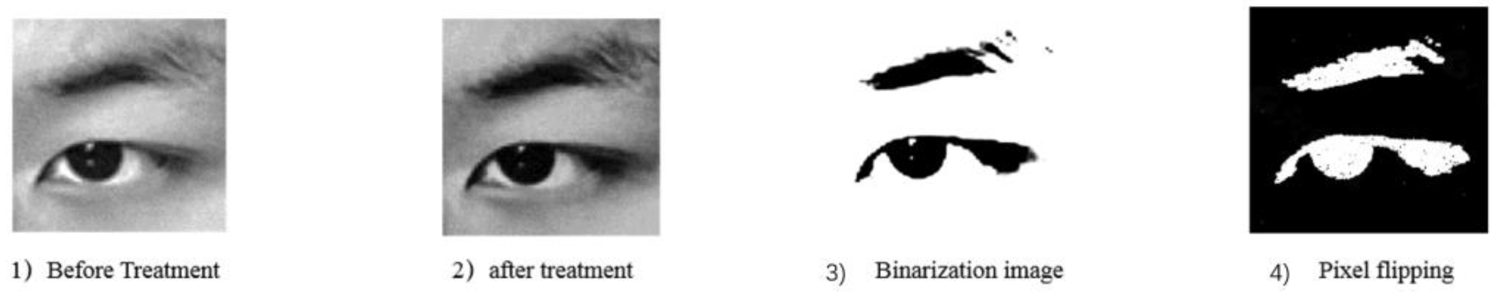
Histogram equalization of an eye image involves adjusting the grayscale used to display the image so as to increase the contrast between the eye, eyebrow, and skin color areas and thereby make these structures more distinct, which will improve the extraction accuracy of the aspect ratio [19]. Figure 2.4a and b show images before and after histogram equalization processing, respectively.
2. Image binarization
Considering the color differences in various parts of the eye image, it is possible to set a grayscale threshold to binarize each part of the image [20]. Through experiments, it was concluded that the processing effect was optimal when the grayscale threshold was between 115 and 127, and so the threshold was set to 121. Figure 2.4c shows the binarized image of the eye, and the negative image in Figure 2.4d is used for further data processing since the target area is the eye.
Figure 4.
Eye image processing: 1) before histogram equalization,2) after histogram equalization, 3) after binarization, and 4) the negative binarized image.
Figure 4.
Eye image processing: 1) before histogram equalization,2) after histogram equalization, 3) after binarization, and 4) the negative binarized image.
3. Calculate eye aspect ratio
Determining the minimum bounding rectangle for the binary image as shown in Figure 5 yields two rectangles of the eyebrow and eye. The lower one is the circumscribed rectangle of the eye, and the height and width of the rectangle correspond to the height and width of the eye.
Height and width of the rectangle are obtained by calculating the pixel positions of the four vertices of the rectangle, with the height-to-width ratio of the eye is calculated as . P80 was selected as our fatigue criterion, and so when the pupil is covered by more than 80% of the eyelid, we consider this to indicate fatigue. The height-to-width-ratio statistics for a large number of human eye images were used to calculate the values of eyes in different states. We defined .23 as a closed-eye state, and as an open-eye state [21]. Figure 2.6 shows the aspect ratio of the eye for different closure states.
4. Calculate the PERCLOS value
The principle for calculating the PERCLOS value based on P80 is as follows: assuming that an eye blink lasts for , where the eyes are open at moments and , and the time when the eyelid covers the pupil for more than 80% is , then the value of PERCLOS is
Considering that the experiments involved analyzing eye-video data, continuous images can be obtained after frame extraction, and so the timescale can be replaced by
fps = 30 with fixed image frames; that is, by analyzing the video of the controller’s control eye over a certain period of time, the total number of images collected in the data is , and the number of closed eyes is , then the value of PERCLOS is
Figure 7 shows that the PERCLOS value (for P80) is positively correlated with the degree of fatigue. Therefore, we can take the PERCLOS value of controllers as the indicator value of their eye fatigue, and quantitatively describe the fatigue state of controllers through PERCLOS (P80).
2.3. Decision-level fatigue-information fusion based on the entropy weight method
The concept of entropy is often used in information theory to characterize the degree of dispersion of a system. According to the theory of the entropy weight method, a higher information-entropy index indicates data with a smaller degree of dispersion, and the smaller the impact of the index on the overall evaluation, the lower the weight [22]. According to this theory, the entropy weight method determines the weight according to the degree of discreteness of the data, and the calculation process is more objective. Therefore, the characteristics of information entropy are often used in comprehensive evaluations of multiple indicators to reasonably weight each indicator.
The main steps of the entropy weight method are as follows:
Normalization of indicators. Assuming that there are samples and indexes, represents the value of the th indicator() corresponding to the th sample (), then the normalized value can be expressed as
where and represent the minimum and maximum values of the indicators, respectively.
2. Calculate the proportion of the th sample value under index :.
3. Calculate the entropy of index . According to the definition of information entropy, the information entropy of a set of data values is
where, when , the information entropy is
4. Calculate the weight of each indicator. After obtaining the information entropy of each index, the weight of each index can be calculated using the following formula:
3. Experiments and Verification
3.1. Data acquisition experiment
The experimental data were collected from the air traffic control simulation laboratory. We used the same type of simulator equipment as Air Traffic Control Bureau to restore the experiment scenario, and invited 6 licensed tower controllers to participate in data collection with the cooperation of Air Traffic Control Bureau.
Specifically, the radar control equipment in the experiment is shown in Figure 8. Key data acquisition equipment includes controller air talk recording equipment, facial data acquisition equipment. Speech data were collected directly from the air talk communication system, and eye-video data were collected using a camera with a resolution of 1280×720 at 30 fps. The person included 3 males and 3 females certificated air traffic controllers of Air Traffic Control Bureau. They are all from East China and have more than three years of controller work experience. All subjects were required to have adequate rest (> 7 hours) every night on rest days, and no food, alcohol or drinks that might affect the experimental results. All experimental personnel were fully familiar with the control simulator system. All subjects were informed of the experiment content and had the right to stop the experiment at any time.
The experiment lasted for one week, and was designed according to the scheduling system in the actual control work. Severe fatigue is less common during the work process of air traffic controllers. We increased the workload appropriately to avoid a significant difference between the amount of data collected in non-fatigued and fatigued states. In the week, 6 controllers were arranged to conduct 24 hours of experiment every day on Monday, Wednesday, Friday and Sunday, and controllers were arranged to have full rest on Tuesday, Thursday and Saturday, and they were required to sleep for more than seven hours. Each experimental day contained six sets of work and six sets of rest of two hours each. Each controller worked for two hours, rested for two hours, and completed the experiment for 24 hours in turn. This experimental design was fully consistent with the characteristics of the actual controller post. On the experimental day, the first group of work experiments were conducted from 0:00 to 2:00 for each controller. After two hours of work, the first group of rest was started from 2:00 to 4:00. At the end of each group of work, each controller was arranged to fill in the Karolinska Sleepiness Scale [23], which took 10 minutes. Rest for 110 minutes. After two hours of work, the controller is scheduled to rest for two hours, which is completely consistent with the actual work schedule of the controller. The controlled work experiment alternated with rest periods, with up to 12 hours of work and 12 hours of rest periods within each working day.
The KSS is a reliable fatigue detection scale, with scores ranging from one to ten reflecting the subject's state from alert to almost unable to maintain clarity. According to the usual practice of KSS, when the questionnaire score is greater than or equal to 7, we determine that the controller is in a state of fatigue. At the end of the experiment, fatigue was determined according to the fatigue scale filled out by each controller, which was used as the label of the test data. After the experiment, we obtained a total of 462 minutes of valid voice data and 29 hours of valid facial video data.
3.2. Experiments on speech-fatigue characteristics
We first combined traditional speech features including the MFCC, short-time-average zero-crossing rate, and maximum Lyapunov index, and verified the effectiveness of the FSVM through the classification accuracy of these features. We extracted the largest Lyapunov exponent in the speech signal using data near-fitting [24] and the characteristics of small-sample data. Figure 9 shows the fusion detection process for multiple speech features.
In order to obtain a clearer understanding of the classification performance of each classifier, we output its relevant parameters, as presented in Table 1.
We selected 2100 speech data (for 3 males and 3 females) from the controller speech database as the training set (comprising 1030 fatigue samples and 980 normal samples) for target feature extraction and analysis. Data collected in the past has been processed as necessary and divided them into short frames with a window function length of 25 ms. The step size between successive windows was set to 10 ms, and the number of filters was 40. According to the feature extraction method, the 12th-order MFCC, short-time-average zero-crossing rate, and maximum Lyapunov exponent were extracted from the speech samples under fatigue and normal conditions. The extraction results were tested statistically to identify which of the above features differed significantly with the fatigue state; the results are presented in Table 2.
After analysis of variance (ANOVA) was performed on three speech features: Short-time-average zero-crossing rate, 12th-order MFCC, and Maximum Lyapunov exponent, the mean ± standard deviation values were shown in the table below.
Table 2 indicates that the three speech features changed significantly with the fatigue state, with p<0.01 for the MFCC and maximum Lyapunov exponent. This indicates that these two features are particularly good at representing the fatigue state of the human body.
In order to verify the usefulness of various speech features in detecting controller fatigue, we combined the features in different ways and used the standard SVM and the improved FSVM to classify and detect each combination. We use the data from the previous database as the training data and the data collected in this experiment as the test data. The two types of speech data are strictly separate for classifiers. The test results after 50% cross-validation are presented in Table 3.
Table 3 indicates that the fatigue classification performance was worse for the short-time-average zero-crossing rate than for the other two features. Combining the three features produced the best classification performance, which was due to the traditional features and nonlinear features complementing each other. Moreover, the table indicates that the improved FSVM classifier had higher accuracy than the traditional SVM, which was due to the optimization of the membership determination method.
3.3. Experiments on eye-fatigue characteristics
The OpenCV software library was used to detect eyes in the images. The human-eye-detection algorithm adopted in this study can accurately determine the eye area in both the open- and closed-eye states.
This study analyzed subimages of the right eyes of the experimenters, and calculated aspect ratio of the eye by applying equalization, binarization, and other processing methods to the images. Among the 3783 eye images extracted, 748 images had values of <0.23, resulting in an eye PERCLOS value of 0.20 for experimenter 1 during this period.
Figure 10.
Extraction and processing of eye-fatigue features.
In order to determine the fatigue value of controllers at different time periods more objectively, the MECD characteristic values of the experimenters during that time period were synchronously calculated according to the longest continuous eye-closure time within a single time period. As the degree of fatigue increases, the eyes become more difficult to open in a closed state, or more difficult to keep open when in an open state, leading to an increase in MECD [25]. Considering that the radar signals used for air traffic control are updated every 4 seconds, we used a 40-second time window to detect the MECD value of the controller during each time period, and included it in the calculation of the eye-fatigue value. We considered that a subject was in a state of fatigue when their eye-fatigue value was >0.3. Therefore, 0.3 is set as the threshold value. When MECD is greater than 0.3, the subject is considered to be in a state of fatigue; when MECD is less than or equal to 0.3, the subject is considered to be in a state of no fatigue. The fatigue state of six air traffic controllers was judged by the threshold method, and the average value was taken. The accuracy of the discrimination results compared with the results of the KSS scale was shown in the following table.
the corresponding accuracy values are listed in Table 4.
The experimental results in Table 4 indicate that the accuracy in identifying fatigue state based on eye characteristics was 83.08%, indicating the usefulness of this parameter in evaluating the fatigue state of controllers.
3.4. Multisource information-fusion fatigue-detection experiment
The speech features were also evaluated numerically. By combining the trained decision model with , we applied sentence-by-sentence detection to the control speech data of each experimenter during each time period. This yielded the proportion of fatigued-speech epochs to the total number of speech epochs during the entire time period, which was used as the characteristic value for that experimenter’s fatigued speech during this time period. The speech-fatigue detection results are presented in Table 5.
According to the theory of the entropy weight method, this study first assigned weights to the speech-fatigue value and eye-fatigue value at the decision level. We calculated the weights of eye indicators and speech indicators of the six experimenters by normalizing the data and calculating the information entropy. The results are presented in Table 6.
Based on the sample data of all experimenters, we averaged the weights of the indicators and used them as comprehensive indicator weights. The final indicator weights for the eye- and speech-fatigue values were 0.56 and 0.44, respectively. Based on the weights of the comprehensive indicators, we could obtain the comprehensive fatigue values of controllers at different time periods. We considered that a comprehensive fatigue value of > 0.2 indicated a state of fatigue. Table 7 presents the comprehensive fatigue results for all experimenters.
The experimental results show that the recognition accuracy of the fatigue state based on integrated features was about 86.0%, which was 2.2% and 3.5% higher than those for eye and speech features, respectively, indicating that the fatigue recognition after fusion was more robust. In the experiment, some samples could not be correctly classified. The reason is that different controllers have different vocal characteristics and facial expression characteristics. It is undeniable that some people’s voice quality, timbre, and features such as eyes are similar to the performance of others when they are fatigued, which makes it difficult for the model to classify correctly. It can be seen that fatigue recognition still has great research potential.
4. Conclusions
This study investigated the fatigue state of controllers by analyzing the relationship between multisource fatigue data. Nonlinear speech signal features were extracted from speech signals using the phase-space reconstruction method based on air–land communication data of controllers. Speech feature fusion of multiple features of speech fatigue was carried out using a fuzzy Support Vector Machine algorithm, and a multidimensional feature vector of speech fatigue was established.
The experimental results show that different speech feature combinations have different recognition accuracy, among which Mel Frequency Cepstral Coefficient + short-time-average zero-crossing rate + maximum Lyapunov index has the highest recognition accuracy. In the case of the fuzzy support vector machine classifier, the accuracy reached 82.5% compared to the evaluation results using the fatigue scale KSS. At the same time, several methods such as the AdaBoost algorithm were applied to the eye data of controllers to obtain the Percentage of Eyelid Closure Time feature values. Combined with Maximum Continuous Eye Closure Duration features, the controllers’ eye-fatigue characteristic values were jointly calculated. The accuracy in identifying fatigue state based on eye characteristics was 83.8%. For voice features and facial features, the initial fatigue results for the speech and eye feature layers were weighted using the entropy weight method, and finally comprehensive controller fatigue characteristic values were obtained through decision-level fusion. The accuracy of fatigue detection method combined with eye and speech features respectively was 86.0%, which was 2.2% and 3.5% higher than those for eye and speech features respectively.
The present research findings can provide theoretical guidance for air traffic management authorities attempting to detect ATC fatigue. They might also be useful as a reference in controller scheduling improvement.
Author Contributions
Conceptualization, L.X., S.M., S.H. and Z.S.; methodology, L.X., S.H.; formal analysis, L.X., S.M., S.H. and Y.N.; validation, S.H. and Y.N.; software L.X. and Y.N; writing—original draft preparation, S.M.; writing—review and editing, L.X. and S.M.; resources, supervision, project administration, funding acquisition, Z.S.
Funding
The authors acknowledge the financial support from the National Natural Science Foundation of China (grant no. U2233208).
Data Availability Statement
These data of this study are available from the corresponding author upon request.
Conflicts of Interest
The author(s) declare(s) that there is no conflict of interest regarding the publication of this paper.
References
- International Air Transport Association. (2020). IATA Forecast Predicts 8.2 billion Air Travelers in 2037. 2018.
- Wu, Q. (2008). Research on Driving Fatigue Detection Method Based on ECG Signal (Doctoral dissertation, Zhejiang University).
- Zhao, C., Zhao, M., Liu, J., & Zheng, C. (2012). Electroencephalogram and electrocardiograph assessment of mental fatigue in a driving simulator. Accident Analysis & Prevention, 45, 83-90. [CrossRef]
- Gold, B., Morgan, N., & Ellis, D. (2011). Speech and audio signal processing: processing and perception of speech and music. John Wiley & Sons.
- Schuller, B., Steidl, S., Batliner, A., Schiel, F., Krajewski, J., Weninger, F., & Eyben, F. (2014). Medium-term speaker states—A review on intoxication, sleepiness and the first challenge. Computer Speech & Language, 28(2), 346-374.
- Milosevic, S. (1997). Drivers' fatigue studies. Ergonomics, 40(3), 381-389. [CrossRef]
- Li, X., Tan, N., Wang, T., & Su, S. (2014, October). Detecting driver fatigue based on nonlinear speech processing and fuzzy SVM. In 2014 12th International Conference on Signal Processing (ICSP) (pp. 510-515). IEEE.
- Tijerina, L., Kiger, S., Rockwell, T., & Wierwille, W. (1996). Heavy Vehicle Driver Workload Assessment: Task 5: Workload Assessment Protocol (No. DOT HS-808 467). United States. Joint Program Office for Intelligent Transportation Systems.
- Koçal, O. H., Yuruklu, E., & Avcibas, I. (2008). Chaotic-type features for speech steganalysis. IEEE Transactions on Information Forensics and Security, 3(4), 651-661.
- Shen, Z., Pan, G., & Yan, Y. (2020). A high-precision fatigue detecting method for air traffic controllers based on revised fractal dimension feature. Mathematical Problems in Engineering, 2020, 1-13. [CrossRef]
- Povinelli, R. J., Johnson, M. T., Lindgren, A. C., Roberts, F. M., & Ye, J. (2006). Statistical models of reconstructed phase spaces for signal classification. IEEE Transactions on Signal processing, 54(6), 2178-2186. [CrossRef]
- McClung, S. N., & Kang, Z. (2016). Characterization of visual scanning patterns in air traffic control. Computational intelligence and neuroscience, 2016. [CrossRef]
- Jo, J., Lee, S. J., Park, K. R., Kim, I. J., & Kim, J. (2014). Detecting driver drowsiness using feature-level fusion and user-specific classification. Expert Systems with Applications, 41(4), 1139-1152. [CrossRef]
- Lindeberg, T. (1998). Feature detection with automatic scale selection. International journal of computer vision, 30, 79-116.
- Turk, M. (1991). A. Pentland Eigenfaces for Recognition Journal of Cognitive Neuroscience, Volume 3, Number 1.
- Rennie, J. D., Shih, L., Teevan, J., & Karger, D. R. (2003). Tackling the poor assumptions of naive bayes text classifiers. In Proceedings of the 20th international conference on machine learning (ICML-03) (pp. 616-623).
- Chang, C. C., & Lin, C. J. (2011). LIBSVM: a library for support vector machines. ACM transactions on intelligent systems and technology (TIST), 2(3), 1-27.
- Sommer, D., & Golz, M. (2010, August). Evaluation of PERCLOS based current fatigue monitoring technologies. In 2010 Annual International Conference of the IEEE Engineering in Medicine and Biology (pp. 4456-4459). IEEE.
- Viola, P., & Jones, M. (2001). Robust real-time object detection. International journal of computer vision, 4(34-47), 4.
- Lienhart, R., & Maydt, J. (2002, September). An extended set of haar-like features for rapid object detection. In Proceedings. international conference on image processing (Vol. 1, pp. I-I). IEEE.
- Xie, J. F., Xie, M., & Zhu, W. (2012, December). Driver fatigue detection based on head gesture and PERCLOS. In 2012 International Conference on Wavelet Active Media Technology and Information Processing (ICWAMTIP) (pp. 128-131). IEEE.
- Sahoo, M. M., Patra, K. C., Swain, J. B., & Khatua, K. K. (2017). Evaluation of water quality with application of Bayes' rule and entropy weight method. European Journal of Environmental and Civil Engineering, 21(6), 730-752. [CrossRef]
- Laverde-López, M. C., Escobar-Córdoba, F., & Eslava-Schmalbach, J. (2022). Validation of the Colombian version of the Karolinska sleepiness scale. Sleep Science, 15(Spec 1), 97.
- Yang Yongfeng, Wu Minjuan, Gao Ku, et al(2012).Parameter selection for calculating the maximum Lyapunov exponent using the small data volume method. Vibration, Testing and Diagnosis, 2012, 32 (3): 371-374.
- Niu, Q. N. (2014). Research on fatigue driving detection method based on information fusion. Jilin University.
Figure 1.
Fatigue-detection scheme based on multilevel information fusion.
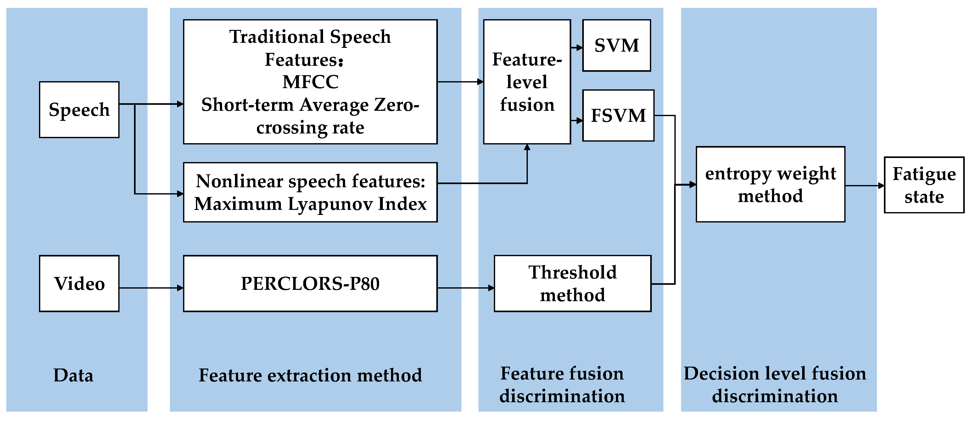
Figure 2.
Schematic diagrams of traditional 1) and normal-plane 2) membership functions.
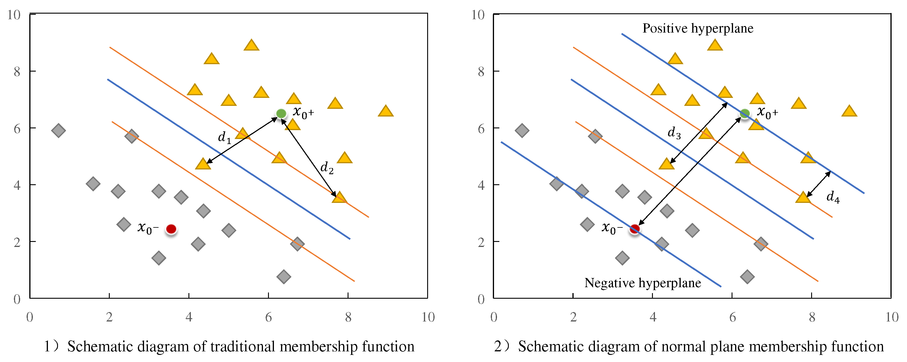
Figure 3.
Images of a human eye in different closure states:1) fully open, 2) partially open,3) almost closed, and 4) fully closed.
Figure 3.
Images of a human eye in different closure states:1) fully open, 2) partially open,3) almost closed, and 4) fully closed.

Figure 5.
Eye minimum bounding rectangle.
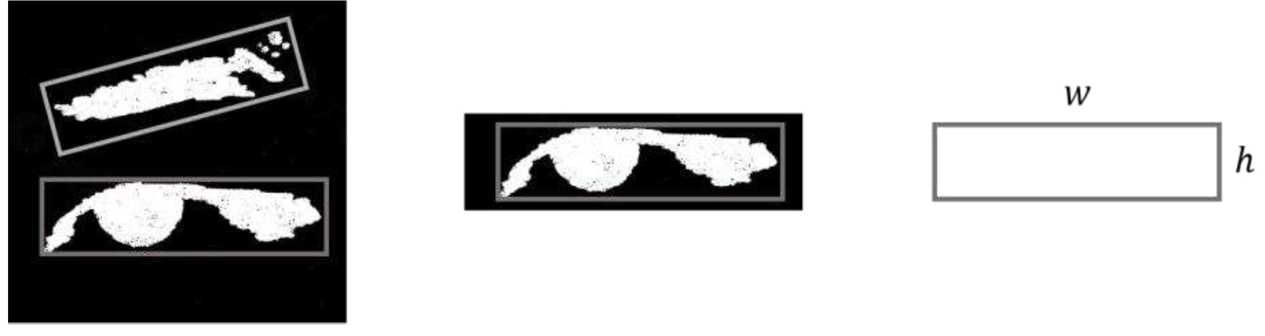
Figure 2.6.
Eye aspect ratios for the closure states shown in Figure 2.3: 1) = 0.35, 2) = 0.32, 3) = 0.17, and 4) = 0.13.
Figure 2.6.
Eye aspect ratios for the closure states shown in Figure 2.3: 1) = 0.35, 2) = 0.32, 3) = 0.17, and 4) = 0.13.
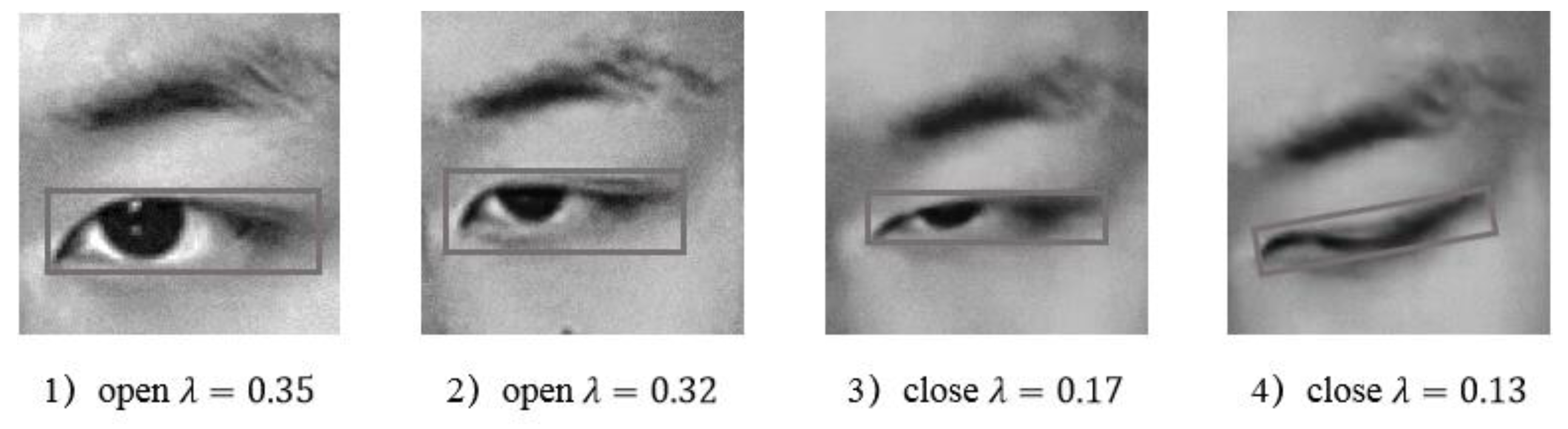
Figure 7.
Relationship between PERCLOS value (for P80) and degree of fatigue.
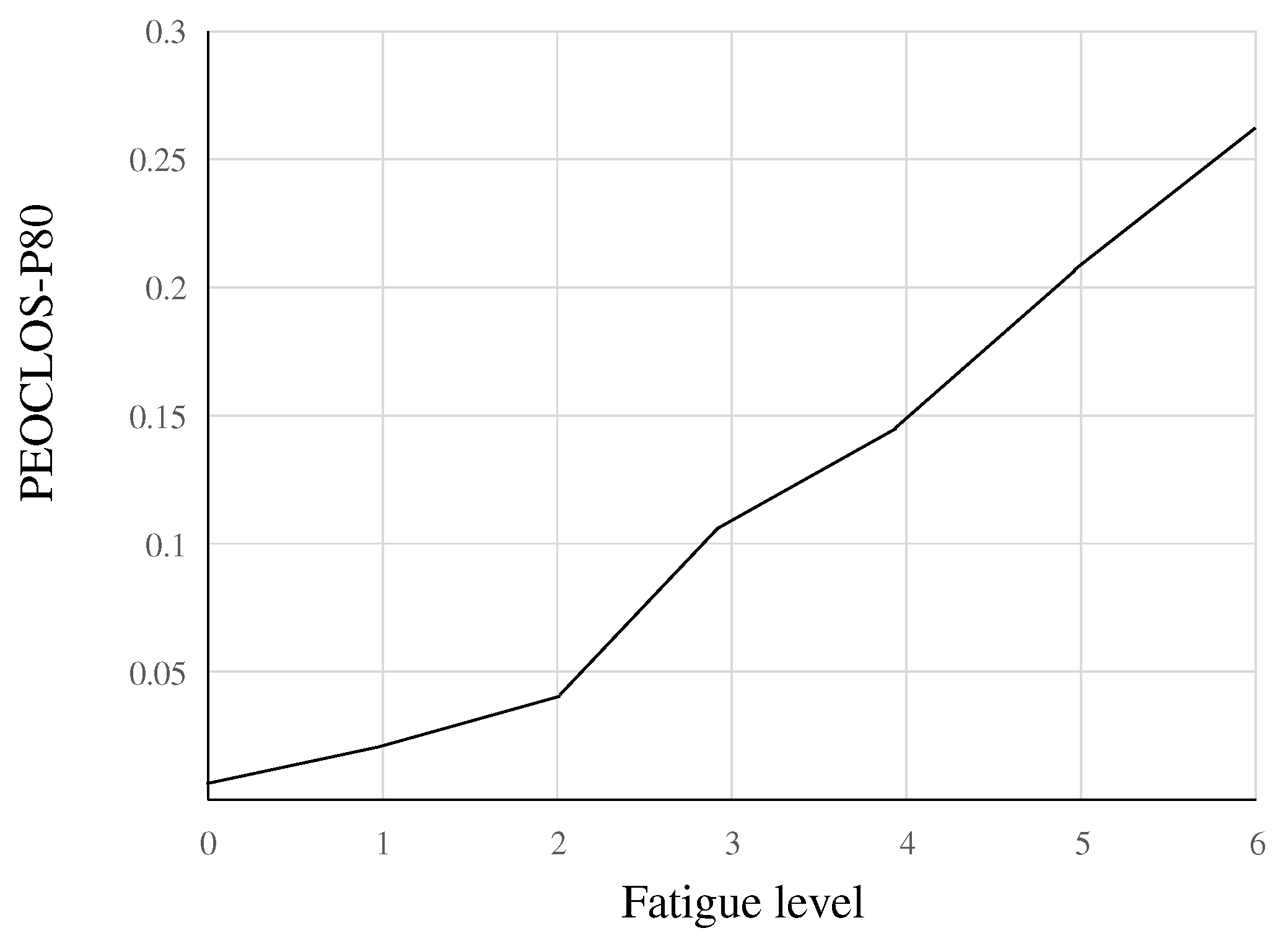
Figure 8.
Experimental environment.
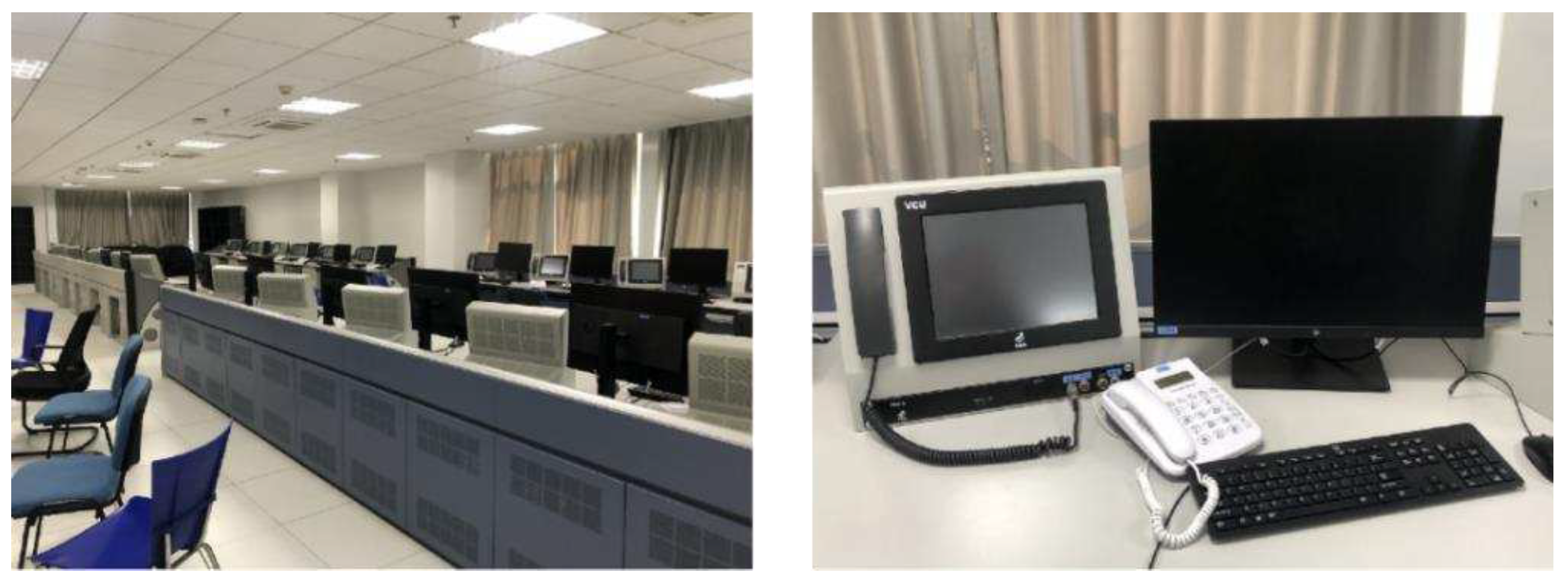
Figure 9.
Speech-fatigue feature detection process.
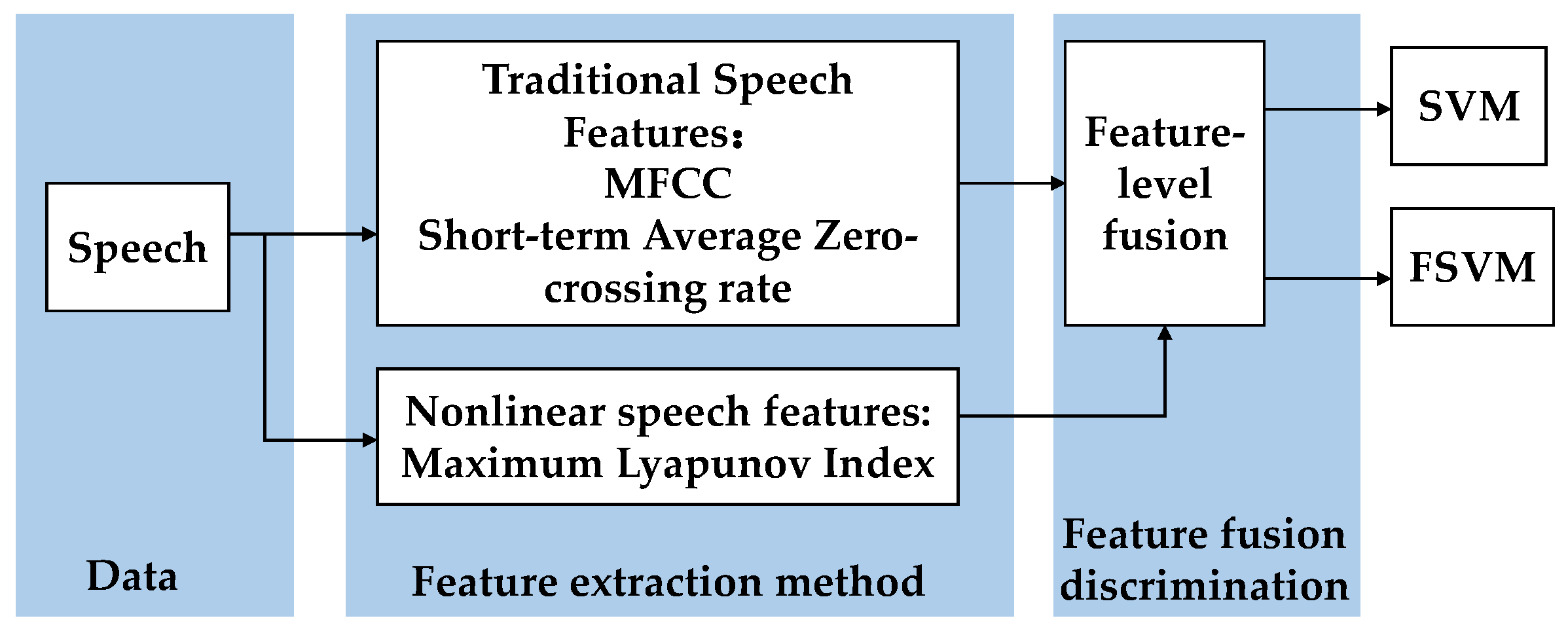

Table 1.
Classifier internal parameters.
| Classification algorithm | Penalty parameter | Kernel-function scaling parameter | Number of support vectors |
| Standard SVM | 64 | 0.0625 | 62 |
| Improved FSVM | 128 | 0.125 | 39 |
Table 2.
Differences in speech features between different states.
| Phonetic feature | Normal sample | Fatigue sample | Significance (p=sig) | |
| Short-time-average zero-crossing rate (times/frame) | 71.46.2 | 66.97.3 | 3.67 | |
| 12th-order MFCC | –0.910.47 | 0.140.51 | 7.62 | |
| Maximum Lyapunov exponent | 0.340.07 | 0.250.05 | 10.2 |
Table 3.
Test results for speech-fatigue characteristics.
| Group | SVM accuracy | FSVM accuracy |
| MFCC + short-time-average zero-crossing rate | 75.4% | 77.1% |
| MFCC + maximum Lyapunov index | 78.3% | 79.5% |
| Short-time-average zero-crossing rate + maximum Lyapunov index | 73.1% | 73.8% |
| MFCC + short-time-average zero-crossing rate + maximum Lyapunov index | 80.4% | 82.5% |
Table 4.
Calculated eye-fatigue values for experimenter.
| Time interval | MECD (s) | Eye-fatigue value | Accuracy |
| 0:00–2:00 | 0.48 | 0.34 | 83.2% |
| 4:00–6:00 | 0.08 | 0.34 | 82.2% |
| 8:00–10:00 | 0.82 | 0.33 | 79.5% |
| 12:00–14:00 | 0.77 | 0.18 | 78.9% |
| 16:00–18:00 | 0.97 | 0.23 | 88.1% |
| 20:00–22:00 | 0.82 | 0.19 | 86.6% |
Table 5.
Speech-fatigue detection results for experimenter 1.
| Time period | Total number of fatigued-speech epochs | Total number of speech epochs | Fatigue value |
| 0:00–2:00 | 23 | 308 | 0.07 |
| 4:00–6:00 | 50 | 290 | 0.17 |
| 8:00–10:00 | 27 | 289 | 0.09 |
| 12:00–14:00 | 53 | 309 | 0.17 |
| 16:00–18:00 | 56 | 274 | 0.20 |
| 20:00–22:00 | 56 | 259 | 0.22 |
Table 6.
Sample weights of the experimenters.
| Experimenter | Eye indicators | Speech indicators |
| 1 | 0.55 | 0.45 |
| 2 | 0.58 | 0.42 |
| 3 | 0.55 | 0.45 |
| 4 | 0.53 | 0.47 |
| 5 | 0.59 | 0.41 |
| 6 | 0.57 | 0.43 |
Table 7.
Recognition accuracy of the comprehensive fatigue value.
| Time period | Comprehensive fatigue value | Accuracy |
| 0:00–2:00 | 0.22 | 84.3% |
| 4:00–6:00 | 0.25 | 85.2% |
| 8:00–10:00 | 0.21 | 81.7% |
| 12:00–14:00 | 0.18 | 89.6% |
| 16:00–18:00 | 0.22 | 84.9% |
| 20:00–22:00 | 0.20 | 90.3% |
Disclaimer/Publisher’s Note: The statements, opinions and data contained in all publications are solely those of the individual author(s) and contributor(s) and not of MDPI and/or the editor(s). MDPI and/or the editor(s) disclaim responsibility for any injury to people or property resulting from any ideas, methods, instructions or products referred to in the content. |
© 2023 by the authors. Licensee MDPI, Basel, Switzerland. This article is an open access article distributed under the terms and conditions of the Creative Commons Attribution (CC BY) license (http://creativecommons.org/licenses/by/4.0/).
Copyright: This open access article is published under a Creative Commons CC BY 4.0 license, which permit the free download, distribution, and reuse, provided that the author and preprint are cited in any reuse.


