Kinetics of Wavefunction Decay: Detection of Photon Entanglement and Realization of Q-bits at Room Temperature

1. Introduction

The notion that quantum mechanics operates as a probabilistic process can be traced back to the research of Nelson [1] and has endured over time. However, Nelson's hypotheses ultimately fell short due to the imposition of a particular stochastic derivative with time-inversion symmetry, which limited its generality. Furthermore, the results of Nelson's theory do not entirely align with those of quantum mechanics, as demonstrated by Von Neumann's proof [2] of the impossibility of hidden variables.

The definitive resolution to this question was provided by Kleinert [3] (refer to Appendix A), who utilized the path integral approach to establish that quantum mechanics can be conceptualized as an imaginary-time probabilistic process. These imaginary-time quantum fluctuations differ from the more commonly understood real-time fluctuations. They result in a "reversible" pseudo-diffusion behavior, which is elucidated by the Madelung quantum hydrodynamic model through the action of the quantum potential.

The distinguishing characteristic of quantum pseudo-diffusion is the impossibility to define a positive diffusion coefficient. This leads to a significant implication: the quantum evolution within spatially distributed system may exhibit local entropy reduction over a certain spatial domains and reversible deterministic evolution with recurrence time and overall null entropy variation [4].

In this study, the author investigates the quantum imaginary-time stochastic process in scenarios where real-time random fluctuations are concurrently in play leading to irreversible quantum evolution and possibly to decoherence and classical behavior on large scale systems. The goal of this work is accomplished by extending the Madelung hydrodynamic description of quantum mechanics to its stochastic counterpart.

The primary topics encompass:

i. Elucidating the formulation of the stochastic quantum hydrodynamic equation of motion as a consequence of fluctuations in spacetime curvature originating from the noisy background of gravitational waves (dark energy).

ii. Exploring the path integral approach to comprehend quantum-stochastic dynamics, which describes the progression of quantum superposition states and potentially their transition to stable configurations.

iii. Describing stationary quantum state configurations in the presence of noise and establishing their correspondence with standard quantum mechanical states.

iv. Defining the circumstances under which the “zero noise” deterministic limit of stochastic theory aligns with conventional quantum mechanics.

v. Identifying the criteria that lead to the emergence of classical behavior within extensive-scale systems.

vi. Generalizing the uncertainty principles within the context of fluctuating quantum systems.

vii. Investigating quantum entanglement, wave function decay and measurement process.

viii. Comparing the measurement process as defined by the stochastic quantum hydrodynamic model with the perspectives of decoherence theory and the Copenhagen interpretation of quantum mechanics.

ix. Examining experiments involving entangled photons within the context of finite time-decay kinetics of wave functions.

x. Extension of quantum coherence to macroscopic distances in order to build up a system with a large number of Q-bits

2. The quantum potential fluctuations induced by the background of stochastic gravitational waves

The quantum-hydrodynamic representation of the Schrodinger equation [5-7]

$$-i\hslash {\partial }_t\psi =\left(\frac{{\hslash }^2}{2m}{\partial }_i{\partial }_i-V_{(q)}\right)\psi$$

(2.1)

for the complex wave function $\psi =\left|\psi \right|{\mathrm{e}}^{-\frac{iS}{\hslash }}$, are given by the conservation equation for the mass density $|\psi {|}^2$

$${\partial }_t|\psi {|}^2+{\partial }_i(|\psi {|}^2{\dot{q}}_i)=0$$

(2.2)

and by the motion equation

$${\ddot{q}}_{j_{(t)}}=-\frac{1}{m}{\partial }_j\left(V_{(q)}+V_{q{u}_{(n)}}\right)$$

(2.3)

where ${\dot{q}}_i$is defined, through the momentum $p_i={\partial }_i{S}_{(q,t)}$, where$S_{(q,t)}=-\frac{\hslash }{2}\ln \frac{\psi }{\psi *}$and where

$$V_{qu}=-\frac{{\hslash }^2}{2m}\frac{1}{\left|\psi \right|}{\partial }_i{\partial }_i\left|\psi \right|$$

(2.4)

In order to introduce the effect of the metric tensor fluctuations of the space-time background, we assume that:

1. The fluctuations of the vacuum curvature are described by the wave function ${\psi }_{vac}$with density $|{\psi }_{vac}{|}^2$;

2. The (dark) energy density $E$ of the gravitational waves is proportional to $|{\psi }_{vac}{|}^2$ ;

3. The equivalent mass of vacuum fluctuations $m_{dark}$is defined by the identity$E=m_{dark}{c}^2|{\psi }_{vac}{|}^2$The stochastic gravitational wrinkles originated by the big-bang and the gravitational dynamics of space-time, are approximately assumed to not interact with the physical system (gravitational interaction is sufficiently weak to be disregarded).

4. In this case the wave function of the overall system ${\psi }_{tot}$ reads

$${\psi }_{tot}\cong \psi {\psi }_{vac}$$

(2.5)

Moreover, by assuming that, the equivalent mass $m_{dark}$ of the dark energy of gravitational waves is much smaller than the mass of the system (i.e., $m_{tot}=m_{dark}+m\cong m$), the overall quantum potential (2.4) reads

$$\begin{array}{l}{V}_{q{u}_{(n_{tot})}}=-\frac{{\hslash }^2}{2m_{tot}}\left|\psi {|}^{-1}\right|{\psi }_{vac}{|}^{-1}{\partial }_i{\partial }_i\left|\psi \right|\left|{\psi }_{vac}\right|=\\ =-\frac{{\hslash }^2}{2m}\left(\left|\psi {|}^{-1}{\partial }_i{\partial }_i\right|\psi |+|{\psi }_{vac}{|}^{-1}{\partial }_i{\partial }_i\left|{\psi }_{vac}\right|+\left|\psi {|}^{-1}\right|{\psi }_{vac}{|}^{-1}{\partial }_i\left|{\psi }_{vac}\right|{\partial }_i\left|\psi \right|\right)\end{array}$$

(2.6)

Moreover, given the vacuum mass density noise of wave-length $\lambda$

$$\delta {\rho }_{vac(\lambda )}=|{\psi }_{vac(\lambda )}{|}^2\propto {\cos }^2\frac{2\pi }{\lambda }q$$

(2.7)

associated to the dark energy fluctuation wave-function

$${\psi }_{vac}\propto \pm \cos \frac{2\pi }{\lambda }q$$

(2.8)

it follows that the quantum potential energy fluctuations read

$$\delta {\overline{E}}_{qu}={\displaystyle \underset{V}{\overset{}{\int }}{n}_{tot}{}_{(q,t)}\delta V_{qu(q,t)}dV}$$

(2.9)

Where

$$\begin{array}{l}\delta V_{qu(q,t)}=-\frac{{\hslash }^2}{2m}\left(\left|{\psi }_{vac}{|}^{-1}{\partial }_i{\partial }_i\right|{\psi }_{vac}|+|\psi {|}^{-1}\left|{\psi }_{vac}{|}^{-1}{\partial }_i\right|{\psi }_{vac}\left|{\partial }_i\right|\psi |\right)\\ =\frac{{\hslash }^2}{2m}\left({\left(\frac{2\pi }{\lambda }\right)}^2+\left|\psi {|}^{-1}{\left(\pm \cos \frac{2\pi }{\lambda }q\right)}^{-1}\left(\pm \sin \frac{2\pi }{\lambda }q\right){\partial }_i\right|\psi |\right)\\ =\frac{{\hslash }^2}{2m}\left({\left(\frac{2\pi }{\lambda }\right)}^2+\left(\tan \frac{2\pi }{\lambda }q\right)\left|\psi {|}^{-1}{\partial }_i\right|\psi |\right)\end{array}$$

(2.10)

For $V\to \infty$ , the unidimensional case leads to

$$\begin{array}{l}\delta {\overline{E}}_{qu(\lambda )}=\frac{1}{{\overline{n}}_{tot}V}\frac{{\hslash }^2}{2m}{\displaystyle \underset{V}{\overset{}{\int }}{\mathrm{n}}_{tot}{}_{(q,t)}\left({\left(\frac{2\pi }{\lambda }\right)}^2+\left(\tan \frac{2\pi }{\lambda }q\right)\left|\psi {|}^{-1}{\partial }_i\right|\psi |\right)dq}\\ =\frac{1}{{\overline{n}}_{tot}V}\frac{{\hslash }^2}{2m}\left({\left(\frac{2\pi }{\lambda }\right)}^2{\displaystyle \underset{V}{\overset{}{\int }}{\mathrm{n}}_{tot}{}_{(q,t)}dq}+{\displaystyle \underset{V}{\overset{}{\int }}{\mathrm{n}}_{tot}{}_{(q,t)}\left(\left(\tan \frac{2\pi }{\lambda }q\right)\left|\psi {|}^{-1}{\partial }_i\right|\psi |\right)dq}\right)\cong \frac{{\hslash }^2}{2m}{\left(\frac{2\pi }{\lambda }\right)}^2\end{array}$$

(2.11)

In (2.11) it has been used the normalization condition ${\displaystyle \underset{V}{\overset{}{\int }}{\mathrm{n}}_{tot}{}_{(q,t)}dq}={\overline{n}}_{tot}V$ and, on large volume ($V\gg {\lambda }_c{}^3$ see (2.15)), it has been used the approximation

$${\lim }_{\lambda \to 0}{\displaystyle \underset{-\infty }{\overset{\infty }{\int }}{\mathrm{n}}_{tot}{}_{(q,t)}\left(\tan \left(\frac{2\pi }{\lambda }q\right)\left|\psi {|}^{-1}{\partial }_i\right|\psi |\right)dq}\ll {\overline{n}}_{tot}V{\left(\frac{2\pi }{\lambda }\right)}^2$$

(2.12)

For the three-dimensional case, (2.11) leads to

$$\delta {\overline{E}}_{qu(\lambda )}\cong \frac{{\hslash }^2}{2m}{\displaystyle \sum _i{\left(k_i\right)}^2}=\frac{{\hslash }^2}{2m}|k{|}^2$$

(2.13)

The result (2.13) shows that the energy, due to the mass/energy density fluctuations of the vacuum, increases as the inverse squared of $\lambda$ . Being so, the quantum potential fluctuations, of very short-wave length (i.e., $\lambda \to 0$) can lead to unlimited large energy fluctuations even for vanishing noise amplitude $T\to 0$. This fact could prevent the realization of the deterministic, zero noise, limit (2.2-4) representing the quantum mechanics.

On the other hand, the convergence to the deterministic limit (2.2-4) of quantum mechanics for $T\to 0$ is warranted by the fact that uncorrelated fluctuations on shorter and shorter distances are energetically unlikely. Thence, the requirement of convergence to the conventional quantum mechanics for $T\to 0$ implies a supplemental condition on the spatial correlation function of the noise as $\lambda \to 0$.

The calculation of the shape of the spatial correlation function of noise, that we name $G(\lambda )$, brings a quite heavy stochastic calculation [8]. A more simple and straight way to calculate $G(\lambda )$ is obtained by considering the spectrum of the fluctuations.

Since each component of spatial frequency $k=\frac{2\pi }{\lambda }$ brings the quantum potential energy contribution (2.11), its probability of happening, reads

$$\begin{array}{l}{p}_{\left(\lambda \right)}\propto \exp \left[-\frac{\delta {\overline{E}}_{qu}}{kT}\right]\\ =\exp \left[-\frac{\frac{{\hslash }^2}{2m}{\left(\frac{2\pi }{\lambda }\right)}^2}{kT}\right]=\exp \left[-{\left(\frac{\pi {\lambda }_c}{\lambda }\right)}^2\right]\end{array}$$

(2.14)

Where

$${\lambda }_c=\sqrt{2}\frac{\hslash }{{(mkT)}^{1/2}}$$

(2.15)

is the De Broglie length.

From (2.14) the spectrum $S(k)$of the spatial frequency reads

$$S(k)\propto p(\frac{2\pi }{\lambda })=\exp \left[-{\left(\frac{\pi {\lambda }_c}{\lambda }\right)}^2\right]=\exp \left[-{\left(\frac{k{\lambda }_c}{2}\right)}^2\right]$$

(2.16)

From (2.16) we can see that the spectrum is not white and the components with wave-length $\lambda$ smaller than ${\lambda }_c$ go quickly to zero. Besides, from (2.16) the spatial shape $G(\lambda )$reads

$$\begin{array}{l}{G}_{(\lambda )}\propto {\displaystyle \underset{-\infty }{\overset{+\infty }{\int }}\exp [ik\lambda ]S_{(k)}dk}\propto {\displaystyle \underset{-\infty }{\overset{+\infty }{\int }}\exp [ik\lambda ]\exp \left[-{\left(k\frac{{\lambda }_c}{2}\right)}^2\right]dk}\\ \propto \frac{{\pi }^{1/2}}{{\lambda }_c}\exp \left[-{\left(\frac{\lambda }{{\lambda }_c}\right)}^2\right]\end{array}$$

(2.17)

The expression (2.17) shows that uncorrelated mass density fluctuations on shorter and shorter distance are progressively suppressed by the quantum potential allowing the realization of the conventional “deterministic” quantum mechanics for systems whose physical length is much smaller than the De Broglie one ${\lambda }_c$.

For the sufficiently general case to be of practical interest, where the mass density noise correlation function can be assumed Gaussian with null correlation time, isotropic into the space and independent among different co-ordinates, it can be assumed of the form

$$<\delta {\mathrm{n}}_{(q_{\alpha },t)},\delta {\mathrm{n}}_{(q_{\beta }+\lambda ,t+\tau )}>=<\delta {\mathrm{n}}_{(q_{\alpha })},\delta {\mathrm{n}}_{(q_{\beta })}{>}_{(T)}G(\lambda )\delta (\tau ){\delta }_{\alpha \beta }$$

(2.18)

that, for system whose physical length $L$ is much smaller than the De Broglie’ one (i.e., $\frac{L}{{\lambda }_c}\ll 1$), reads

$$G_{(\lambda )}\propto \frac{1}{{\lambda }_c}\exp \left[-{\left(\frac{\lambda }{{\lambda }_c}\right)}^2\right]\cong \frac{1}{{\lambda }_c}\left(1-{\left(\frac{\lambda }{{\lambda }_c}\right)}^2\right)\cong \frac{1}{{\lambda }_c}=\frac{1}{\hslash }\sqrt{\frac{mkT}{2}}$$

(2.19)

On this ansatz, equation (2.3) assumes the stochastic form [9] (see appendix B)

$${\ddot{q}}_{j_{(t)}}=-\kappa {\dot{q}}_{j_{(t)}}-\frac{1}{m}\frac{\partial \left(V_{(q)}+V_{q{u}_{(\rho )}}\right)}{\partial q_j}+\kappa D_{}^{1/2}{\xi }_{(t)}$$

(2.20)

where [9]

$$D^{1/2}=\left(\frac{L}{{\lambda }_c}\right){\left({\gamma }_D\frac{\hslash }{2m}\right)}^{1/2}=\sqrt{{\gamma }_D}\frac{L}{2}\sqrt{\frac{kT}{2\hslash }}$$

(2.21)

where ${\gamma }_D$ is a pure not zero number [9].

It is worth noting that the probability mass density function $\rho$ is now defined by the Smolukowski conservation equation stemming from (2.20) and obeys to the condition ${\lim }_{T\to 0}\rho =|\psi {|}^2$since by (2.17-18) the convergence to the quantum mechanics is warranted.

The gravitational dark energy introduces the concept of a self-fluctuating system where the noise is an intrinsic property that does not require the presence of an environment.

3. The Langevin-Schrodinger equation from the Stochastic Madelung quantum Hydrodynamics

Generally assuming for the stochastic case, the complex field

$${\psi }_{\left(q,t\right)}={\rho }_{(q,t)}{}^{1/2}\exp \left[i\frac{S_{\left(q,t\right)}}{\hslash }\right]$$

(3.21)

where close to the deterministic limit of quantum mechanics we can utilize the identity${\rho }_{(q,t)}{}^{1/2}\cong \left|{\psi }_{\left(q,t\right)}\right|$, it follows that the quantum-hydrodynamic equations (2.2-4) reads

$$\begin{array}{l}{\ddot{q}}_i=\frac{1}{m}\frac{d}{dt}{\partial }_{i}S={\partial }_t{\partial }_{i}S+\frac{1}{m}\left({\partial }_i{\partial }_{j}S\right){\partial }_{j}S={\partial }_i\left({\partial }_{t}S+\frac{1}{m}{\partial }_{j}S{\partial }_{j}S\right)\\ =-\frac{1}{m}{\partial }_i\left(V_{(q)}-\frac{{\hslash }^2}{2m}\frac{1}{\left|\psi \right|}{\partial }_j{\partial }_j\left|\psi \right|+\kappa S-q_{{}_j}^{1/2}{q}_{{}_j}^{1/2}m\kappa D^{1/2}{\xi }_{(t)}\right)\end{array}$$

(3.22)

leading to the partial stochastic differential equation

$$m{\partial }_{t}S+{\partial }_{i}S{\partial }_{i}S=-\left(V_{(q)}-\frac{{\hslash }^2}{2m}\frac{1}{\left|\psi \right|}{\partial }_j{\partial }_j\left|\psi \right|+\kappa S-q_{{}_j}^{1/2}{q}_{{}_j}^{1/2}m\kappa D^{1/2}{\xi }_{(t)}+C_{(t)}\right)$$

(3.23)

Equation (3.23) leads to the Langevin-Schrodinger equation, by observing that, for system of physical length $L$ (such as $\frac{L}{{\lambda }_c}\ll 1$ ), $\rho$ obeys to the Smolukowski conservation equation (see Equations (C.24-27) in appendix C) that reads

$$\begin{array}{l}{\lim }_{\frac{L}{{\lambda }_c}\to 0}\left({\partial }_t{n}_{(q,t)}+{\partial }_i\left(n_{(q,t)}<\dot{q}{>}_i\right)+Q_{dis{s}_{(q,t)}}\right)\\ \cong {\lim }_{\frac{L}{{\lambda }_c}\to 0}\left({\partial }_{t}n+{\partial }_{i}n{\dot{q}}_i+Q_{dis{s}_{(q,t)}}\right)=0\end{array}$$

(3.24)

where${\rho }_{(q,t)}={\displaystyle \underset{}{\overset{}{\int }}N(q,p,t)}{d}^{3}p$ (see (C.21, C.22-7) in appendix C) and

$$Q_{dis{s}_{(q,t)}}={\displaystyle \underset{}{\overset{}{\int }}\left(\begin{array}{c}0\\ \frac{1}{2}\frac{\partial D{N}_{(q,p,t)}}{\partial p_{\alpha }}+\dots +\frac{1}{n!}{\displaystyle \sum _{h=2}^{\infty }\frac{{\partial }^k{C}_{{}_{\alpha \chi \mathrm{........}\epsilon }}^{(k)}{N}_{(q,p,t)}}{\underset{(k-terms)}{\underbrace{\partial p_{\chi }\dots \partial p_{\epsilon }}}}}\end{array}\right)d^{3h}p}$$

(3.25)

In fact, since close to the deterministic limit of quantum mechanics it holds that

$${\lim }_{\frac{{\lambda }_c}{L}\to \infty }<\dot{q}>=\dot{q}$$

(3.26)

where $<\mathrm{....}>$ stands for the mean value, and

$${\lim }_{\frac{{\lambda }_c}{L}\to \infty }\rho ={|\psi |}^2$$

(3.27)

it follows that

$${\partial }_t\left|\psi \right|=-\frac{1}{m}{\partial }_i\left|\psi \right|{\partial }_{i}S-\frac{1}{2m}\left|\psi \right|{\partial }_i{\partial }_{i}S+\frac{Q_{dis{s}_{(q,t)}}}{2\left|\psi \right|}$$

(3.28)

Equation (3.28) with the help of (3.23), leads to the generalized Langevin-Schrodinger equation (GLSE) that for time-independent systems reads

$$-i\hslash {\partial }_t\left|\psi \right|=\frac{{\hslash }^2}{2m}{\partial }_i{\partial }_i\psi -\left(V_{(q)}+Const+\kappa S-q_{{}_i}^{1/2}{q}_{{}_i}^{1/2}m\kappa D^{1/2}{\xi }_{(t)}+i\frac{Q_{dis{s}_{(q,t)}}}{2|\psi {|}^2}\right)\psi$$

(3.29)

Close to the deterministic limit of quantum mechanics (i.e., microscopic system with physical length $L$much smaller than ${\lambda }_c$) it is possible to characterize the ability of the system to dissipate by the semiempirical parameter $\alpha$defined by the relation [9] ${\lim }_{{}_{\frac{L}{{\lambda }_c}\to 0}}\kappa \cong {\lim }_{T\to 0}\alpha \frac{2kT}{mD}$. On this ansatz, the realization of the quantum mechanics is warranted (see Equation (2.20)) by the condition ${\lim }_{{}_{\frac{L}{{\lambda }_c}\to 0}}\alpha =0$. In this case, it can be readily seen that the GLSE (3.29) reduces to the Schrodinger equation.

When the parameter $\alpha$ remains quite high close to quantum limit such as

$${\lim }_{\frac{L}{{\lambda }_c}\to 0}\alpha ={\alpha }_0$$

(3.30)

Equation (3.29) converges to the quantum Brownian motion. In fact, under condition (3.30) and by utilizing dimensional considerations, the following identities apply:

$$\mathrm{I}.{\lim }_{{}_{\frac{L}{{\lambda }_c}\to 0}}D={\lim }_{T\to 0}{\gamma }_D{\left(\frac{L}{{\lambda }_c}\right)}^{{}^2}\frac{\hslash }{2m}={\lim }_{T\to 0}{\gamma }_D{L}^2\frac{kT}{4\hslash }=0$$

(3.31)

$$\mathrm{II}.{\lim }_{{}_{\frac{L}{{\lambda }_c}\to 0}}\kappa \cong {\lim }_{T\to 0}\alpha \frac{2kT}{mD}={\alpha }_0\frac{8\hslash }{m{\gamma }_D{L}^2}=finite$$

(3.32)

$$\mathrm{III}.{\lim }_{{}_{\frac{L}{{\lambda }_c}\to 0}}{Q}_{dis{s}_{(q,t)}}=0$$

(3.33)

Thus, by (3.32-33) being$\left|\frac{Q_{dis{s}_{(q,t)}}}{2|\psi {|}^2}\right|<<\left|\kappa S\right|$, the term $i\frac{Q_{dis{s}_{(q,t)}}}{|\psi {|}^2}$ can be disregarded in (3.29) and close to the deterministic limit (i.e.,$\frac{L}{{\lambda }_c}\ll 1$) it follows the conventional Langevin equation for the quantum Brownian motion

$${\lim }_{T\to 0}i\hslash {\partial }_t\psi =-\frac{{\hslash }^2}{2m}{\partial }_i{\partial }_i\psi +\left(V_{(q)}+\kappa S-q_{{}_i}^{1/2}{q}_{{}_i}^{1/2}m\kappa D^{1/2}{\xi }_{(t)}+C\right)\psi$$

(3.34)

4. The quantum path integral motion equation in presence of stochastic noise

The Markov process (3.21) obeys the Smolukowski integro-differential equation for the Markov probability transition function (PTF) [10]

$$P(q,q_0|t+\tau ,t_0)={\displaystyle \underset{-\infty }{\overset{\infty }{\int }}P(q,z|\tau ,t)P(z,q_0|t-t_0,t_0)}{d}^{r}z$$

(4.1)

(4.1)

where the PTF $P(q,z|\tau ,t)$ represents the probability that a quantity of the probability mass density (PMD) $\rho (q,t)$ at instant t, in a time interval τ, in a point z, is transferred to the point q [10].

The conservation of the PMD $\rho$ in integral form shows that the PTF generates the displacement of a vector (q,t) – (z,0) according to the rule [10]

$$\rho (q,t)={\displaystyle \underset{}{\overset{}{\int }}P(q,z|t,0){\rho }_{(z,0)}}{d}^{r}z$$

(4.2)

Generally speaking, for the quantum case, equation (4.1) cannot be reduced to a Fokker-Planck equation (FPE), since the quantum potential $V_{qu}{}_{{}_{(\rho )}}$ owns a functional dependence by ${\rho }_{(q,t)}$ and the PTF $P(q,q_0|t+\tau ,t_0)$ is non-Gaussian (see Appendix C ) .

Nonetheless, if the initial distribution ${\rho }_{(q,t_0)}$ is stationary (e.g., quantum eigenstate) and is close to the long-time final stationary distribution ${\rho }_{eq}$ of the stochastic case, it is possible to assume that the quantum potential is constant in time as a Hamilton potential following the approximation

$$V_{qu}=-(\frac{{\hslash }^2}{4m})\left({\partial }_q{\partial }_q\ln {\rho }_{eq}{}_{(q)}+\frac{1}{2}{\left({\partial }_q\ln {\rho }_{eq}{}_{(q)}\right)}^2\right)$$

(4.3)

Being in this case the quantum potential fixed and independent by the wave function, the PMD $\rho$the stationary long-time solution is given by the Fokker-Plank equation

$${\partial }_t\frac{\partial }{\partial t}{P}_{(q,z|t,0)}+{\partial }_p{P}_{(q,z|t,0)}\upsilon =0$$

(4.4)

Where

$$\upsilon =-\frac{1}{m\kappa }{\partial }_q\left(V_{(q)}-\frac{{\hslash }^2}{4m}\left({\partial }_q{\partial }_q\ln {\rho }_{eq}{}_{(q)}+\frac{1}{2}{\left({\partial }_q\ln {\rho }_{eq}{}_{(q)}\right)}^2\right)\right)-\frac{D}{2}{\partial }_q\ln {\rho }_{eq}$$

(4.5)

leading to the final equilibrium of the stationary quantum configuration

$$\frac{1}{m\kappa }{\partial }_q\left(V_{(q)}-\frac{{\hslash }^2}{4m}\left({\partial }_q{\partial }_q\ln {\rho }_{eq}{}_{(q)}+\frac{1}{2}{\left({\partial }_q\ln {\rho }_{eq}{}_{(q)}\right)}^2\right)\right)+\frac{D}{2}{\partial }_q\ln {\rho }_{eq}=0$$

(4.6)

In Appendix D the stationary states of linear systems obeying to (4.6) are shown. The results show that the quantum eigenstates are stable and maintains their shape (with a small change of their variance) when subject to fluctuations.

4.1. Evolution of quantum superposition of states submitted to stochastic noise

In order to determine the evolution of quantum superposition of states, that are not stationary, (not considering fast kinetics and jumps) we have to integrate the stochastic differential equation (2.20) that eliminating fast variables reads

$$\dot{q}=-{\gamma }_D\frac{L^2}{8\alpha \hslash }{\partial }_q\left(V_{(q)}-\frac{{\hslash }^2}{4m}\left({\partial }_q{\partial }_q\ln {\rho }_{(q.t)}+\frac{1}{2}{\left({\partial }_q\ln {\rho }_{(q,t)}\right)}^2\right)\right)+\sqrt{{\gamma }_D}\frac{L}{2}\sqrt{\frac{kT}{\hslash }}{\xi }_{(t)}$$

(4.7)

As shown below, this can be done by using the discrete approach with the help of both the Smolukowski integro-differential equation (4.1) and the associated conservation equation (4.2) for the PMD $\rho$.

We integrate the SDE (4.7) by using its 2^nd order discrete expansion

$$q_{k+1}\cong q_k-\frac{1}{m\kappa }{\partial }_k\left(V_{(q_k)}+V_{qu({\rho }_{q_k,}{t}_k)}\right)\Delta t_k-\frac{1}{m\kappa }\frac{d}{dt}{\partial }_k\left(V_{(q_k)}+V_{qu({\rho }_{q_k,}{t}_k)}\right)\frac{\Delta t_k{}^2}{2}+D_{}^{1/2}\Delta W_k$$

(4.8)

where

$$q_k=q_{(t_k)}$$

(4.9)

$$\Delta t_k=t_{k+1}-t_k$$

(4.10)

$$\Delta W_k=W_{{}_{(t_{k+1})}}-W_{{}_{(t_k)}}$$

(4.11)

where $\Delta W_k$ has Gaussian zero mean and unitary variance whose probability function $P(\Delta W_k,\Delta t)$, for $\Delta t_k=\Delta t\forall k$, reads

$$\begin{array}{l}{\lim }_{\Delta t\to 0}P(\Delta W_k,\Delta t)={\lim }_{\Delta t\to 0}{\left(4\pi D\Delta t\right)}^{-1/2}\exp -\frac{\Delta W_k{}^2}{4\Delta t}\\ ={\lim }_{\Delta t\to 0}{\left(4\pi D\Delta t\right)}^{-1/2}\exp -\frac{1}{4\Delta t}\frac{{\left(q_{k+1}-<q_{k+1}>\right)}^2}{D}\\ ={\left(4\pi D\Delta t\right)}^{-1/2}\exp -\frac{1}{4\Delta t}\frac{{\left(q_{k+1}-q_k-<{\dot{\overline{q}}}_k>\Delta t-\frac{<{\ddot{\overline{q}}}_k>}{2}\Delta t^2\right)}^2}{D}\end{array}$$

(4.12)

where it has been introduced the midpoint approximation

$${\overline{q}}_k=\frac{q_{k+1}+q_k}{2}$$

(4.13)

and where

$$<{\dot{\overline{q}}}_k>=-\frac{1}{m\kappa }\frac{\partial \left(V_{({\overline{q}}_{{}_k})}+V_{qu({\rho }_{{\overline{q}}_{{}_k}}{t}_k)}\right)}{\partial {\overline{q}}_k}$$

(4.14)

and

$$<{\ddot{\overline{q}}}_k>=-\frac{1}{2m\kappa }\frac{d}{dt}\frac{\partial \left(V_{({\overline{q}}_{{}_k})}+V_{qu({\rho }_{({\overline{q}}_k)},t_k)}\right)}{\partial {\overline{q}}_k}$$

(4.15)

are the solutions of the deterministic problem:

$$<q_{k+1}>\cong <q_k>-\frac{1}{m\kappa }{\partial }_k\left(V_{(q_k)}+V_{qu({\rho }_{q_k,}{t}_k)}\right)\Delta t_k-\frac{1}{m\kappa }\frac{d}{dt}{\partial }_k\left(V_{(q_k)}+V_{qu({\rho }_{q_k,}{t}_k)}\right)\frac{\Delta t_k{}^2}{2}$$

(4.16)

By using standard manipulations [3], from (4.12), the PTF reads

$$\begin{array}{l}P(q,q_0,t,t_0)=P(q_n,q_0|t-t_0,0)={\lim }_{\Delta t\to 0}P(q_n,q_0|n\Delta t,0)\\ ={\lim }_{\Delta t\to 0}{\displaystyle \underset{-\infty }{\overset{\infty }{\int }}{\prod }_{k=1}^{n}d{q}_{k-1}P(q_k,q_{k-1}|\Delta t,(k-1)\Delta t)}\\ ={\lim }_{\Delta t\to 0}\left\{{\prod }_{k=1}^n{\displaystyle \underset{-\infty }{\overset{\infty }{\int }}d{q}_{k-1}}\right\}{\left(4\pi D\Delta t\right)}^{-n/2}\exp \left[\begin{array}{l}-\frac{1}{2D}{\displaystyle \sum _{k=1}^n<{\dot{\overline{q}}}_{k-1}>\Delta q_k}-\frac{\Delta t}{4D}{\displaystyle \sum _{k=1}^n\begin{array}{l}{\left(\frac{q_k-q_{k-1}}{\Delta t}\right)}^2\\ +<{\dot{\overline{q}}}_{k-1}{>}^2\end{array}}\\ -\frac{\Delta t}{4D}{\displaystyle \sum _{k=1}^n{D}^{1/2}\Delta W_k<{\ddot{\overline{q}}}_{k-1}{>}_{(q_{k-1})}}\end{array}\right]\\ ={\displaystyle \underset{q_0}{\overset{q}{\int }}Dq}\exp \left[-\frac{1}{2D}{\displaystyle \sum _{k=1}^n<{\dot{\overline{q}}}_{k-1}>\Delta q_k}\right]\exp -\frac{\Delta t}{4D}\left[{\displaystyle \sum _{k=1}^n\begin{array}{l}{\left(\frac{q_k-q_{k-1}}{\Delta t}\right)}^2+<{\dot{\overline{q}}}_{k-1}{>}^2\\ -2D\frac{\partial <{\dot{\overline{q}}}_{k-1}>}{\partial {\overline{q}}_{k-1}}\end{array}}\right]\\ =\left(\exp {\displaystyle \underset{q_0}{\overset{q}{\int }}\frac{1}{2D}<\dot{q}{>}_{(q,t)}dq}\right){\displaystyle \underset{q_0}{\overset{q}{\int }}Dq}\exp -\frac{1}{4D}{\displaystyle \underset{t_0}{\overset{t}{\int }}dt\left({\dot{q}}^2+<\dot{q}{>}^2+2D{\partial }_q<\dot{q}>\right)}\end{array}$$

(4.17)

where it has been introduced the discrete PTF $P(q_k,q_{k-1}|\Delta t,(k-1)\Delta t)$ that reads

$$\begin{array}{l}{\lim }_{\Delta t\to 0}P(q_k,q_{k-1}|\Delta t,(k-1)\Delta t)={\lim }_{\Delta t\to 0}{\left(4\pi D\Delta t\right)}^{-1/2}\exp \frac{\Delta t}{2D}\left[\begin{array}{l}-<{\dot{\overline{q}}}_{k-1}>\left(\frac{q_k-q_{k-1}}{\Delta t}\right)\\ -\frac{1}{2}\left(\begin{array}{l}{\left(\frac{q_k-q_{k-1}}{\Delta t}\right)}^2+<{\dot{\overline{q}}}_{k-1}{>}^2\\ -2D\frac{\partial <{\dot{\overline{q}}}_{k-1}>}{\partial {\overline{q}}_{k-1}}\end{array}\right)\end{array}\right]\\ ={\lim }_{\Delta t\to 0}{\left(4\pi D\Delta t\right)}^{-1/2}\exp \frac{\Delta t}{4D}\left[-{\left({\dot{q}}_{k-1}-<{\dot{\overline{q}}}_{k-1}>\right)}^2+2D\frac{\partial <{\dot{\overline{q}}}_{k-1}>}{\partial {\overline{q}}_{k-1}}\right]\end{array}$$

(4.18)

Before proceeding further, we observe that, generally speaking, since the quantum potential is a function of the PMD

$$\rho (q_k,t_k)={\displaystyle \underset{-\infty }{\overset{\infty }{\int }}P(q_k,q_0|t_k,0)\rho (q_0,0)}d{q}_0$$

(4.19)

the evolution of equation (4.8) depends on the exact sequence of the noise inputs $D_{}^{1/2}\Delta W_k$and, therefore, also on the discrete time interval of integration. This behavior can be easily verified by performing the numerical integration of (4.8). The vagueness of the problem can be analytically identified by the fact that, $<{\dot{\overline{q}}}_{k-1}{>}_{\left(<{\dot{q}}_k>\right)}$and $\frac{\partial <{\dot{\overline{q}}}_{k-1}{>}_{\left(<{\dot{q}}_k>\right)}}{\partial q_{k-1}}$depend on $\rho (q_k,k\Delta t)$ and $\rho (q_{k+1},\left(k+1\right)\Delta t)$, that define the quantum potential values $V_{q{u}_{({\rho }_k)}}$, $V_{q{u}_{({\rho }_{k+1})}}$ , unknown at the time instant $\left(k-1\right)\Delta t$.

Although there is no general solution to this problem, in the limit of small speed ${\dot{q}}_k$ and small noise amplitude, it is possible to proceed by successive steps of approximation since the existence of the deterministic limit (see appendix E)

$${\lim }_{\Delta t\to 0}{\lim }_{D\to 0}{\dot{q}}_k={\lim }_{\Delta t\to 0}<{\dot{\overline{q}}}_k>=<{\dot{q}}_k>$$

(4.20)

warrants that, for sufficiently short time interval$\Delta t$, the speed change is small enough to have that

$$\frac{<{\dot{q}}_{k+1}>}{<{\dot{q}}_k>}=1+<\epsilon >$$

(4.21)

with $<\epsilon >\ll 1$, and that

$$<{\dot{\overline{q}}}_k>=\frac{<{\dot{q}}_{k+1}>+<{\dot{q}}_k>}{2}=<{\dot{q}}_k>\left(1+\frac{<\epsilon >}{2}\right)\cong <{\dot{q}}_k>$$

(4.22)

Therefore, by starting from the zero order of approximation $<{\dot{\overline{q}}}_k>\cong <{\dot{q}}_k>$, there exists a sufficiently small noise amplitude, as well as small diffusion coefficient $D={\gamma }_D\frac{L^2}{4}\frac{kT}{\hslash }$ , to obtain the PTF by successive steps of approximation where the starting zero one reads

$$\begin{array}{l}{P}^{(0)}(q_k,q_{k-1}|\Delta t,(k-1)\Delta t)\\ ={\left(4\pi D\Delta t\right)}^{-1/2}\exp \frac{\Delta t}{4D}\left[-{\left({\dot{q}}_{k-1}-\frac{<{\dot{q}}_k>+<{\dot{q}}_{k-1}>}{2}\right)}^2+D\frac{\partial <{\dot{q}}_k>+<{\dot{q}}_{k-1}>}{\partial {\overline{q}}_{k-1}}\right]\\ ={\left(4\pi D\Delta t\right)}^{-1/2}\exp \frac{\Delta t}{4D}\left[-{\left({\dot{q}}_{k-1}-<{\dot{q}}_{k-1}>\left(1+\frac{<\epsilon >}{2}\right)\right)}^2+D\frac{\partial <{\dot{q}}_k>+<{\dot{q}}_{k-1}>}{\partial {\overline{q}}_{k-1}}\right]\\ \cong {\left(4\pi D\Delta t\right)}^{-1/2}\exp \frac{\Delta t}{4D}\left[-{\left({\dot{q}}_{k-1}-<{\dot{q}}_{k-1}>\right)}^2+2D{\partial }_{q_{k-1}}<{\dot{q}}_{k-1}>\right]\end{array}$$

(4.23)

which can be used to find the zero order of approximation of the PMD $n$ at the next instant k

$${\rho }^{(0)}(q_k,k\Delta t)={\displaystyle \underset{-\infty }{\overset{\infty }{\int }}{P}^{(0)}(q_k,q_{k-1}|\Delta t,\left(k-1\right)\Delta t)\rho (q_{k-1},\left(k-1\right)\Delta t)}d{q}_{k-1}$$

(4.24)

and find the approximated zero-order quantum potential at the instant k that allows to obtain

$$<{\dot{q}}_k{>}^{(0)}=-\frac{1}{m\kappa }{\partial }_{q_{{}_k}}\left(V_{(q_{{}_k})}-\frac{{\hslash }^2}{4m}\left({\partial }_q{\partial }_q\ln {\rho }^{(0)}{}_{(q_{{}_k},t_k)}+\frac{1}{2}{\left({\partial }_q\ln {\rho }^{(0)}{}_{(q_{{}_k},t_k)}\right)}^2\right)\right)$$

(4.25)

Thence, at the next order of approximation, the PTF and the associated PMD read, respectively,

$$\begin{array}{l}{P}^{(1)}(q_k,q_{k-1}|\Delta t,(k-1)\Delta t)\\ ={\left(4\pi D\Delta t\right)}^{-1/2}\exp \frac{\Delta t}{4D}\left[-{\left({\dot{q}}_{k-1}-\frac{<{\dot{q}}_k{>}^{(0)}+<{\dot{q}}_{k-1}>}{2}\right)}^2+D\frac{\partial <{\dot{q}}_k{>}^{(0)}+<{\dot{q}}_{k-1}>}{\partial {\overline{q}}_{k-1}}\right]\\ \cong {\left(4\pi D\Delta t\right)}^{-1/2}\exp \frac{\Delta t}{4D}\left[-{\left({\dot{q}}_{k-1}-\frac{<{\dot{q}}_k{>}^{(0)}+<{\dot{q}}_{k-1}>}{2}\right)}^2+2D\left({\partial }_{q_k}<{\dot{q}}_k{>}^{(0)}+{\partial }_{q_{k-1}}<{\dot{q}}_{k-1}>\right)\right]\end{array}$$

(4.26)

and

$${\rho }^{(1)}(q_k,k\Delta t)={\displaystyle \underset{-\infty }{\overset{\infty }{\int }}{P}^{(1)}(q_k,q_{k-1}|\Delta t,\left(k-1\right)\Delta t)\rho (q_{k-1},\left(k-1\right)\Delta t)}d{q}_k$$

(4.27)

that leads to the mean velocity

$$<{\dot{q}}_k{>}^{(1)}=-\frac{1}{m\kappa }{\partial }_{q_k}\left(V_{(q_{{}_k})}-\frac{{\hslash }^2}{4m}\left({\partial }_q{\partial }_q\ln {\rho }^{(1)}{}_{(q_{{}_k},t_k)}+\frac{1}{2}{\left({\partial }_q\ln {\rho }^{(1)}{}_{(q_{{}_k},t_k)}\right)}^2\right)\right)$$

(4.28)

Thence, repeating the procedure, at successive u-th order of approximation (u=2, ,3, .......r) we obtain

$$\begin{array}{l}{P}^{(u)}(q_k,q_{k-1}|\Delta t,(k-1)\Delta t)\\ ={\left(4\pi D\Delta t\right)}^{-1/2}\exp \frac{\Delta t}{4D}\left[-{\left({\dot{q}}_{k-1}-\frac{<{\dot{q}}_k{>}^{(u-1)}+<{\dot{q}}_{k-1}>}{2}\right)}^2+D\frac{\partial <{\dot{q}}_k{>}^{(u-1)}+<{\dot{q}}_{k-1}>}{\partial {\overline{q}}_{k-1}}\right]\\ \cong {\left(4\pi D\Delta t\right)}^{-1/2}\exp \frac{\Delta t}{4D}\left[-{\left({\dot{q}}_{k-1}-\frac{<{\dot{q}}_k{>}^{(u-1)}+<{\dot{q}}_{k-1}>}{2}\right)}^2+D\left({\partial }_{q_k}<{\dot{q}}_k{>}^{(u-1)}+{\partial }_{q_{k-1}}<{\dot{q}}_{k-1}>\right)\right]\end{array}$$

(4.29)

and

$${\rho }^{(u)}(q_k,k\Delta t)={\displaystyle \underset{-\infty }{\overset{\infty }{\int }}{P}^{(u)}(q_k,q_{k-1}|\Delta t,\left(k-1\right)\Delta t)\rho (q_{k-1},\left(k-1\right)\Delta t)}d{q}_k$$

(4.30)

$$<{\dot{q}}_k{>}^{(u)}=-\frac{1}{m\kappa }{\partial }_{q_k}\left(V_{(q_{{}_k})}-\frac{{\hslash }^2}{4m}\left({\partial }_q{\partial }_q\ln {\rho }^{(u)}{}_{(q_{{}_k},t_k)}+\frac{1}{2}{\left({\partial }_q\ln {\rho }^{(u)}{}_{(q_{{}_k},t_k)}\right)}^2\right)\right)$$

(4.31)

so that the final PTF $P^{(\infty )}(q_k,q_{k-1}|\Delta t,(k-1)\Delta t)$ reads

$$\begin{array}{l}{P}^{(\infty )}(q_k,q_{k-1}|\Delta t,(k-1)\Delta t)={\lim }_{u\to \infty }{P}^{(u)}(q_k,q_{k-1}|\Delta t,(k-1)\Delta t)\\ \cong {\left(4\pi D\Delta t\right)}^{-1/2}\exp \frac{\Delta t}{4D}\left[-{\left({\dot{q}}_{k-1}-\frac{<{\dot{q}}_k{>}^{(\infty )}+<{\dot{q}}_{k-1}>}{2}\right)}^2+D\left({\partial }_{q_k}<{\dot{q}}_k{>}^{(\infty )}+{\partial }_{q_{k-1}}<{\dot{q}}_{k-1}>\right)\right]\end{array}$$

(4.32)

It worth noting that the convergence of (4.32) generally depends by the chaoticity of the classical trajectories of motion of the system, by the amplitude of the noise $T$ and by the discrete time interval $\Delta t$.

Nonetheless, the existence of the deterministic limit of quantum mechanics warrants the existence of the basin of convergence of (4.32) in the$\lim \left(T,\Delta t\right)\to 0$.

If, given the discrete values of $\left(T,\Delta t\right)$, $P^{(u)}$oscillates and ${\lim }_{u\to \infty }{P}^{(u)}$ cannot be precisely determined within the framework of a numerical procedure, we can regularize the PTF $P^{(u)}$ by taking its mean values starting from the $\overline{u}-th$ order of approximation such as

$$P^{(\infty )}={\lim }_{u\to \infty }\mathrm{Re}g\left\{P^{(u)}\right\}={\lim }_{u\to \infty }\frac{1}{u-\overline{u}+1}{\displaystyle \sum _{i=\overline{u}}^u{P}^{(i)}}$$

(4.33)

Finally, the PMD at the $k$-th instant reads

$${\rho }^{(\infty )}(q_k,k\Delta t)={\displaystyle \underset{-\infty }{\overset{\infty }{\int }}{P}^{(\infty )}(q_k,q_{k-1}|\Delta t,(k-1)\Delta t)\rho (q_{k-1},\left(k-1\right)\Delta t)}d{q}_{k-1}$$

(4.34)

leading to the velocity field

$$<{\dot{q}}_k{>}^{(\infty )}=-\frac{1}{m\kappa }{\partial }_{q_k}\left(V_{(q_{{}_k})}-\frac{{\hslash }^2}{4m}\left({\partial }_q{\partial }_q\ln {\rho }^{(\infty )}{}_{(q_{{}_k},t_k)}+\frac{1}{2}{\left({\partial }_q\ln {\rho }^{(\infty )}{}_{(q_{{}_k},t_k)}\right)}^2\right)\right)$$

(4.35)

Moreover, the continuous PTF reads

$$\begin{array}{l}P(q,q_0|t-t_0,0)={\lim }_{\Delta t\to 0}{P}^{(\infty )}(q_n,q_0|n\Delta t,0)\\ ={\lim }_{\Delta t\to 0}{\displaystyle \underset{-\infty }{\overset{\infty }{\int }}{\prod }_{k=1}^{n}d{q}_{k-1}{P}^{(\infty )}(q_k,q_{k-1}|\Delta t,(k-1)\Delta t)}\\ ={\displaystyle \underset{q_0}{\overset{q}{\int }}Dq}\exp \left[-\frac{1}{2D}{\displaystyle \sum _{k=1}^n<{\dot{\overline{q}}}_{k-1}{>}^{(\infty )}\Delta q_k}\right]\exp -\frac{\Delta t}{4D}\left[{\displaystyle \sum _{k=1}^n\begin{array}{l}{\left(\frac{q_k-q_{k-1}}{\Delta t}\right)}^2+<{\dot{\overline{q}}}_{k-1}{>}^{(\infty )}{}^{{}^2}\\ -2D\frac{\partial <{\dot{\overline{q}}}_{k-1}{>}^{(\infty )}}{\partial {\overline{q}}_{k-1}}\end{array}}\right]\\ =\left(\exp {\displaystyle \underset{q_0}{\overset{q}{\int }}\frac{1}{2D}<\dot{q}{>}_{(q,t)}dq}\right){\displaystyle \underset{q_0}{\overset{q}{\int }}Dq}\exp -\frac{1}{4D}{\displaystyle \underset{t_0}{\overset{t}{\int }}dt\left({\dot{q}}^2+<\dot{q}{>}^{{}^2}+2D{\partial }_q<\dot{q}>\right)}\end{array}$$

(4.36)

where$<{\dot{\overline{q}}}_{k-1}{>}^{(\infty )}=\frac{<{\dot{q}}_k{>}^{(\infty )}+<{\dot{q}}_{k-1}{>}^{(\infty )}}{2}$.

The general solution, given in the recursive formula (4.36), can be applied also to non-linear system that cannot be treated by standard approaches [11-14].

4.2. General features of relaxation of quantum superposition of states

In the classical case, the Brownian process described by the FPE admits the stationary long-time solution

$$P(q,q_{-\infty }|t-t_{-\infty },t_{-\infty })={\lim }_{t_0\to -\infty }N\exp \frac{1}{D}{\displaystyle \underset{q_{-\infty }}{\overset{q}{\int }}<\dot{q}{>}_{(q{’}_{{}_{\left(t,t_0\right)}})}dq’}=N\exp \frac{1}{D}{\displaystyle \underset{q_{-\infty }}{\overset{q}{\int }}K(q’)dq’}$$

(4.37)

where$K(q)=-\frac{1}{m\kappa }\frac{\partial V_{(q)}}{\partial q}$leading to the canonical expression [3]

$$P(q,q_0|t-t_0,t_0)=\left(\exp {\displaystyle \underset{q_0}{\overset{q}{\int }}\frac{1}{2D}K(q’)dq’}\right){\displaystyle \underset{q_0}{\overset{q}{\int }}Dq}\exp -\frac{1}{4D}{\displaystyle \underset{t_0}{\overset{t}{\int }}dt\left({\dot{q}}^2+K^2(q)+2D{\partial }_{q}K(q)\right)}$$

(4.38)

Generally speaking, in the quantum case (4.36), $<\dot{q}{>}^{(\infty )}{}_{(q,t)}$ cannot be given in a closed form (4.37) since it depends on the specific relaxation path ${\rho }_{(q,t)}$ of the system toward the steady state which significantly depends on the initial conditions ${\rho }_{(q,t_0)}$ ,$<\dot{q}{>}_{(q,t_0)}$and, therefore, on the initial time $t_0$ when the quantum superposition of states are submitted to fluctuations.

Besides, from (4.8) we can see that $q_{t_k}$depends by the exact sequence of inputs of stochastic noise since, in classically chaotic systems, very small differences can lead to relevant divergences of the trajectories in a short time. Thus, in principle, different long-period stationary configurations ${\rho }_{(q,t=\infty )}$ (i.e., eigenstates) can be reached whenever starting from identical superposition of states. Being so, in classically chaotic systems, the Born’s rule can be applied also to the measure of the single quantum state.

Even if $L\ll {\lambda }_c\cup {\lambda }_{qu}$ , it is worth noting that, in order to have finite quantum lengths ${\lambda }_c$and ${\lambda }_{qu}$ (necessary to the have the quantum-stochastic dynamics of Equation (4.7) and the quantum decoupled (classical) environment or measuring apparatus) the non-linearity of the system-environment interaction is necessary: Quantum decoherence, leading to the decay of superposition states, is significantly promoted by the widespread classical chaotic behavior observed in real systems

On the other hand, a perfect linear universal system would maintain quantum correlations on global scale and would never allow the quantum decoupling between the system and the measuring apparatus necessary for the measure process (see § 4.8). It should be noted that even the quantum decoupling of the system from the environment would be impossible, as quantum systems function as a unified whole. Merely assuming the existence of separate system and environment subtly introduces a classical condition into the nature of the overall supersystem.

Furthermore, since the connection (B.11 ) between the PMD and the MDD holds only at leading order of approximation of $\dot{q}$ (i.e., slow relaxation process and small amplitude of fluctuations), in the case of a large fluctuation (that can occur on time scale much longer than the relaxation one) ${\rho }_{(q,t)}{}_{(q,t)}$ can make transitions not described by (4.36) even from a stationary eigenstate to a generic superposition of states. In this case a new relaxation toward different stationary eigenstate will follow: The PMD ${\rho }_{(q,t)}$ (4.34) describes the relaxation process occurring in the time interval between two large fluctuations, rather than the entire evolution of the system towards a statistical mixture. Because of the long-time-scale of these jumping processes, a system composed of a large number of particles (or independent subsystems) gradually relaxes towards a statistical mixture, with its distribution determined by the temperature dependence of the diffusion coefficient.

5. Emerging classical mechanics on large size systems

Is matter of fact that, if the quantum potential is canceled by hand in the quantum hydrodynamic equations of motion (2.1-3), the classical equation of motion emerges [7]. Even if this is true, this operation is not mathematically correct since it changes the characteristics of the quantum hydrodynamic equations. In fact, doing so, the stationary configurations (i.e., eigenstates) are wiped out because we cancel the balancing force of the quantum potential against the Hamiltonian one [15] that establishes the stationary condition. Thence, an even small quantum potential cannot be neglected into the deterministic quantum hydrodynamic model (2.2-2.4).

Conversely, in the stochastic generalization it is possible to correctly neglect the quantum potential in (2.20, 4.7) when its force is much smaller than the force noise $\varpi$ such as $\left|\frac{1}{m}{\partial }_i{V}_{qu(\rho )}\right|\ll \left|{\varpi }_{(q,t,T)}\right|$that by (4.7) leads to

$$\left|\frac{1}{m}{\partial }_i{V}_{qu(\rho )}\right|\ll \kappa \left(\frac{L}{{\lambda }_c}\right){\left({\gamma }_D\frac{\hslash }{2m}\right)}^{1/2}=\kappa \left(\frac{L\sqrt{mkT}}{2\hslash }\right){\left({\gamma }_D\frac{\hslash }{2m}\right)}^{1/2}$$

(5.01)

and hence, in a coarse-grained description with elemental cell side $\Delta q$, to

$${\lim }_{q\to \Delta q}|{\partial }_i{V}_{qu(\rho )}|\ll m\kappa \left(\frac{L}{{\lambda }_c}\right){\left({\gamma }_D\frac{\hslash }{2m}\right)}^{1/2}=m\kappa \sqrt{{\gamma }_D}\frac{L}{2}\sqrt{\frac{kT}{2\hslash }}$$

(5.02)

where $L$ is the physical system length.

Besides, even if the noise ${\varpi }_{(q,t,T)}$ has zero mean, the mean of the quantum potential fluctuations ${\overline{V}}_{st(\mathrm{n},\mathrm{S})}\cong \kappa S$ is not null so that the dissipative force $-\kappa {\dot{q}}_{{}_{(t)}}$in (6.22) appears. Therefore, the stochastic sequence of inputs of noise alters the coherent evolution of the quantum superposition of state. Moreover, by observing that the stochastic noise

$$\kappa \left(\frac{L}{{\lambda }_c}\right){\left({\gamma }_D\frac{\hslash }{2m}\right)}^{1/2}{\xi }_{(t)}$$

(5.03)

grows with the size of the system, it follows that for macroscopic systems (i.e., $\frac{L}{{\lambda }_c}\to \infty$), condition (5.01) is satisfied if

$${\lim }_{\frac{q}{{\lambda }_c}\to \frac{L}{{\lambda }_c}=\infty }|\frac{1}{m}{\partial }_i{V}_{qu({\mathrm{n}}_{(q)})}|<\infty$$

(5.04)

Actually, in order to have a large-scale description, completely free from quantum correlations, we can more strictly require

$${\lim }_{\frac{q}{{\lambda }_c}\to \infty }|\frac{1}{m}{\partial }_i{V}_{qu({\rho }_{(q)})}|={\lim }_{\frac{q}{{\lambda }_c}\to \infty }\frac{1}{m}\sqrt{{\partial }_i{V}_{qu({\rho }_{(q)})}{\partial }_i{V}_{qu({\rho }_{(q)})}}=0$$

(5.05)

Thus, by observing that for linear systems

$${\lim }_{q\to \infty }{V}_{qu(q)}\propto q^2$$

(5.06)

it straight follows that they cannot lead to the macroscopic classical phase.

Generally speaking, stronger the Hamiltonian potential higher the wave function localization and larger the quantum potential behavior at infinity. This can be easily proven by observing that given the MDD

$$|\psi {|}^2\propto \exp \left[-P^k{}_{(q)}\right]$$

(5.07)

where $P^k{}_{(q)}$ is a polynomial of order k, in order to have a finite quantum potential range of interaction, it must result $k<\frac{3}{2}$. Therefore, linear systems, with $k=2$, own an infinite range of action of quantum potential.

A physical example comes from solids owning a quantum lattice. If we look at phenomena on intermolecular distance where the interaction is linear, the behavior is quantum (e.g., the x-ray diffraction), but if we look at macroscopic properties since the Lennard-Jones potential goes to zero to infinity and the quantum range of interaction is finite (see § 5.1) the classical behavior can emerge since (e.g., low-frequency acoustic wave whose wavelength is much larger than the linear range of interatomic distance).

For instance, for gas phases with particles that interact by Lennard-Jones potential, whose long-distance wave function reads [16]

$${\lim }_{r\to \infty }\left|\psi \right|\propto a^{-1/2}\frac{1}{r}$$

(5.08)

the quantum potential reads

$${\lim }_{r\to \infty }{V}_{qu(\rho )}\cong {\lim }_{q\to \infty }\frac{{\hslash }^2}{2m}\frac{1}{\left|\psi \right|}{\partial }_r{\partial }_r\left|\psi \right|=\frac{1}{r^2}=\frac{{\hslash }^2}{m}a|\psi {|}^2$$

(5.09)

leading to the quantum force

$${\lim }_{r\to \infty }-{\partial }_r{V}_{qu(\rho )}={\lim }_{q\to \infty }\frac{{\hslash }^2}{2m}{\partial }_r\frac{1}{\left|\psi \right|}{\partial }_r{\partial }_r\left|\psi \right|=\frac{{\hslash }^2}{2m}{\partial }_{r}r{\partial }_r{\partial }_r\frac{1}{r}=-2\frac{{\hslash }^2}{m}\frac{1}{r^3}=0$$

(5.10)

so that by (5.01, 5.05), the large-scale classical behavior can appear [17-18] in a sufficiently rarefied phase (see § 5.1-2).

It is interesting to note that in (5.09) the quantum potential is at the basis of the hard sphere potential of the “pseudo potential Hamiltonian model” of the Gross-Pitaevskii equation [19-20] where $\frac{a}{4\pi }$is the boson-boson s-wave scattering length.

By observing that, in order to fulfill the condition (5.05) we can sufficient require that

$${\displaystyle \underset{0}{\overset{\infty }{\int }}{r}^{-1}|\frac{1}{m}{\partial }_i{V}_{qu({\rho }_{(q)})}{|}_{(r,\theta ,\phi )}dr}\text{<}\infty \forall \theta ,\phi$$

(5.11)

so that it is possible to define the quantum potential range of interaction ${\lambda }_{qu}$ as [17-18]

$${\lambda }_{qu}={\lambda }_c\frac{{\displaystyle \underset{0}{\overset{\infty }{\int }}{r}^{-1}|{\partial }_i{V}_{qu({\rho }_{(q)})}{|}_{(r,\theta ,\phi )}dr}}{|{\partial }_i{V}_{qu({\rho }_{(q)})}{|}_{(r={\lambda }_c,\theta ,\phi )}}={\lambda }_c{I}_{qu}$$

(5.12)

that gives a measure of the physical length of the quantum non-local interactions.

For L-J potentials the convergence of the integral (5.11) for $r\to 0$ is warranted since, at short distance the L-J interaction is linear (i.e., ${\lim }_{q\to 0}{V}_{qu({\mathrm{n}}_{(q)})}\propto q^2$) and

$${\lim }_{r\to 0}{r}^{-1}|{\partial }_i{V}_{qu({\rho }_{(q)})}{|}_{(r,\theta ,\phi )}<\infty$$

(5.13)

5.1. Lindemann constant for quantum lattice to classical fluid transition

For a system of Lennard-Jones interacting particles, the quantum potential range of interaction ${\lambda }_{qu}$reads

$${\lambda }_{qu}\cong {\displaystyle \underset{0}{\overset{d}{\int }}dq}+{\lambda }_c{}^4{\displaystyle \underset{d}{\overset{\infty }{\int }}\frac{1}{q^4}dq}=d+\frac{{\lambda }_c}{3}{\left(\frac{{\lambda }_c}{d}\right)}^3$$

(5.14)

where $d=r_0\left(1+\epsilon \right)$ is the distance up to which the interatomic force is approximately linear ($\epsilon =\frac{\Delta }{r_0}$) and where $r_0$ is atomic equilibrium distance.

An experimental confirmation of the physical relevance of quantum potential length of interaction comes from the quantum to classical transition in crystalline solid at melting point when the system passes from a quantum lattice to a fluid amorphous classical phase.

Assuming that, in the quantum lattice, the atomic wave-function (around the equilibrium distance$r_0$) spans itself less than the quantum coherence distance, it follows that at the melting point its variance equals ${\lambda }_{qu}-r_0$.

On these assumptions, the Lindemann constant $L_C=\frac{\left\{\begin{array}{l}\mathrm{wave}\mathrm{function}\mathrm{variance}\\ \mathrm{at}\mathrm{transition}\end{array}\right\}}{r_0}$ [21] reads $L_C=\frac{{\lambda }_{qu}-r_0}{r_0}$ and it can be theoretically calculated since

$${\lambda }_{qu}\approx r_0\left(\left(1+\epsilon \right)+\frac{1}{3}{\left(\frac{{\lambda }_c}{r_0\left(1+\epsilon \right)}\right)}^3\right)\approx r_0\left(\left(1+\epsilon \right)+\frac{1}{3}{\left(\frac{{\lambda }_c}{r_0}\right)}^3\right)$$

(5.15)

that, being typically $\epsilon \approx 0,05÷0,1$ and $\frac{{\lambda }_c}{r_0}\approx 0,8$, leads to

$$L_C=\frac{{\lambda }_{qu}-r_0}{r_0}\approx 0,217÷0,267$$

(5.16)

More accurate evaluation, making use of the potential well approximation for the molecular interaction [17-18], leads to ${\lambda }_{qu}\cong 1,2357{\mathrm{r}}_0$ and to the value of $L_C=0,2357$for the Lindemann constant that well agrees with the measured ones, ranging between 0,2 and 0,25 [21].

5.2. Fluid-superfluid ${}^{4}He$

transition

Since the De Broglie distance ${\lambda }_c$ is a function of temperature, its influence on the fluid-superfluid transition in monomolecular liquids at very low temperature, such as for the ${}^{4}He$,can be detected. The treatment of this case is detailed in ref. [17-18] where, for the ${}^{4}He$ -${}^{4}He$ interaction, the potential well is assumed to be

$$V_{\left(r\right)}=\infty 0<r<\sigma$$

(5.17)

$$V_{\left(r\right)}=-0,82\mathrm{U}\sigma <r<\sigma +2\Delta$$

(5.18)

$$V_{\left(r\right)}=0\sigma +2\Delta <r$$

(5.19)

where ${\mathrm{U}=10,9\mathrm{k}}_B=1,5\times {10}^{-22}J$ is the Lennard-Jones potential deepness, where $\Delta =1,54\times {10}^{.-10}m$and where $\sigma +\Delta =3,7\times {10}^{.-10}m$ is the mean ${}^{4}He$ -${}^{4}He$ atomic distance.

By posing that at superfluid transition the de Broglie length reaches the ${}^{4}He$ -${}^{4}He$ atomic distance and reads

$$\sigma <{\lambda }_c<\sigma +2\Delta$$

(5.20)

we have, for ${\lambda }_c<\sigma$, that the ratio of superfluid/normal ${}^{4}He$ density is about null, while for ${\lambda }_c\approx \sigma +2\Delta$we have almost 100% of superfluid ${}^{4}He$. Therefore, at the condition

$${\lambda }_c=\sqrt{2}\frac{\hslash }{{(mk{T}_{{\lambda }_c})}^{1/2}}=\sigma +\Delta$$

(5.21)

when the superfluid/normal ${}^{4}He$ density ratio is at 50%, it follows that the temperature $T_{50\%}$, for the ${}^{4}He$ mass of $m_{{}^{4}He}=6.6\times {10}^{.-27}kg$, reads

$$T_{50\%}=\frac{2{\hslash }^2}{mk}{\left(\frac{1}{\sigma +\Delta }\right)}^2=\frac{2\times 1,113\times {10}^{.-68}}{6.6\times {10}^{.-27}\times 1,38\times {10}^{.-23}}\left(\frac{1}{1,3\times {10}^{.-19}}\right)=1,92°K$$

(5.22)

that well agrees with the experimental data in ref. [22] of about $1,95°K$.

On the other hand, since by (5.20) for${\lambda }_c=\sigma +2\Delta$ all the couples of ${}^{4}He$ falls into the quantum state, the superfluid ratio of 100% is reached at the temperature

$$T_{100\%}\approx \frac{2{\hslash }^2}{mk}{\left(\frac{1}{\sigma +2\Delta }\right)}^2=0,92°K$$

(5.23)

well agreeing with the experimental data in ref. [22] of about $1,0°K$.

Moreover, by utilizing the superfluid ratio of 38% at the $\lambda$-point of${}^{4}He$, the transition temperature $T_{\lambda }$ reads

$$T_{\lambda }\approx \frac{2{\hslash }^2}{mk}{\left(\frac{1}{\sigma +0,76\Delta }\right)}^2=2,20°K$$

(5.24)

in good agreement of the measured ${}^{4}He$ superfluid transition temperature of $2,17°K$.

It’s worth noting, as a final remark, that there are two ways to establish quantum macroscopic behavior. One approach involves lowering the temperature, which effectively increases the De Broglie length. The second approach is to enhance the strength of the Hamiltonian interaction among the particles within the system.

As far as it concerns the latter, it’s important to note that the limited strength of the Hamiltonian interaction over long distances is the key factor that allows classical behavior to manifest. When we examine systems governed by a quadratic or stronger Hamiltonian potential, the range of interaction associated with the quantum potential becomes infinite, as illustrated in equation (5.44) consequently, achieving a classical phase becomes unattainable, regardless of the system’s size being ${\lambda }_{\infty }=\infty$.

In this particular scenario, we exclusively observe the complete manifestation of classical behavior on a macroscopic scale within systems featuring interactions that are sufficiently weak, weaker even than linear interactions, which are classically chaotic. In this case, the quantum potential lacks the ability to exert its non-local influence over extensive distances.

Therefore, classical mechanics emerges as a decoherent outcome of quantum mechanics when there is a fluctuating spacetime in play.

5.3. The coarse-grained approach

Given the PMD current $J_j{}_{(q,t)}={\rho }_{(q,t)}{\dot{q}}_{j_{(t)}}$, that reads

$$\begin{array}{l}{J}_i{}_{(q,t)}=\rho {\dot{q}}_i{}_{{}_{(t)}}=-\rho \left(\frac{m{L}^2}{4\alpha }{\partial }_i\left(V_{(q)}+V_{qu}\right)+{\varpi }_{(q,t,T)}\right)\\ =-\rho \left(\frac{1}{m\kappa }{\partial }_i\left(V_{(q)}+V_{qu}\right)+D_{jk}^{1/2}{\xi }_{k(t)}\right)\end{array}$$

(5.25)

The macroscopic behavior can be obtained by the discrete coarse-grained spatial description of (5.25), with local cell of side $l$ , that as a function of the j-th cell reads [23]

$$d{x}_j=-\frac{m{L}^2}{4\alpha }D{’}_{jm}{x}_{(m)}\left(D_{mk}{V}_k+D_{{}_{mk}}^{qu}{V}_{q{u}_{{}_k}}\right)dt+D’{’}_{jk}{x}_{(k)}{\Phi }_{(k)}d{W}_k{}_{(t)}$$

(5.26)

where

$$x_j=l^3{\rho }_{(q_j,t)}$$

(5.27)

$$V_k=V_{(q_k)}$$

(5.28)

$$V_{{}_{q{u}_k}}=V_{qu}{}_{({\rho }_{(q_k)})}$$

(5.29)

$${\Phi }_k={\Phi }_{(q_k,t)}$$

(5.30)

where

$${\lim }_{l\to 0}{l}^{-6}<{\Phi }_j,{\Phi }_k>=<{\varpi }_{(q_j)},{\varpi }_{(q_k)}{>}_{(T)}{F}_{(l(k-j))}$$

(5.31)

where$F_{(k-j)}$ is the spatial correlation length of the noise, where the terms$D_{jk}$, $D{’}_{jk}$, $D’{’}_{jk}$ and $D_{{}_{mk}}^{qu}$ are matrices of coefficients corresponding to the discrete approximation of the derivatives $\frac{\partial }{\partial q_k}$at the j-th point.

Generally speaking, the quantum potential interaction $V_{q{u}_k}$stemming by the k-th cell, depends by the strength of the Hamiltonian potential $V_{(q_k)}$ .

By setting, in a system of a huge number of particles, the side length $l$ equal to the mean intermolecular distance$L$, we can have the classical rarefied phase if $L$ is much bigger than the quantum potential length of interaction${\lambda }_{qu}$(that by (5.12)) is also a function of the De Broglie length).

Typically, for the Lennard-Jones potential (5.10) leads to

$${\lim }_{\frac{q}{{\lambda }_{qu}}\to \frac{L}{{\lambda }_{qu}}=\infty }-\frac{\partial V_{qu(\rho )}}{\partial q}\approx 2\frac{{\hslash }^2}{m{\lambda }_{qu}{}^3}\frac{1}{{\left(\frac{q}{{\lambda }_{qu}}\right)}^3}\approx \frac{kT}{\hslash }\sqrt{\frac{mkT}{2}}{I}_{qu}\frac{1}{{\left(\frac{q}{{\lambda }_{qu}}\right)}^3}=0$$

(5.32)

so that the interaction of the quantum potential (stemming by the k-th cell) into the adjacent cells is null and $D_{{}_{mk}}^{qu}$ is diagonal. Thus, the quantum effects are confined into each single molecular cell domain.

Furthermore, being for classical systems $L\gg {\lambda }_c\cup {\lambda }_{qu}$it follows that the spatial correlation length of the noise reads $G_{(k-j)}\propto {\delta }_{kj}$ and the fluctuations appears spatially uncorrelated in the macroscopic systems

Conversely, given that for stronger than linearly interacting systems ${\lambda }_{qu}\to \infty$ and the quantum potential of each cell extends its interaction to the other ones, the quantum character appears on the coarse-grained description.

As shown in §5.2, by using the stochastic hydrodynamic model (SQHM) it is possible to derive descriptions for dense phases where quantum effects appear on macroscopic scale.

5.4. Measurement process and the finite range of non-local quantum potential interaction

Throughout the process of measurement, consisting of “deterministic” conventional quantum interaction between the sensing component of the experimental setup and the system being measured, the interaction ceases when the measuring apparatus is moved to a significant distance away from the system, well beyond the distances${\lambda }_c$and${\lambda }_q$.

The interpretation and handling of the "interaction output" are subsequently managed by the measuring apparatus, typically involving a classical, irreversible procedure characterized by a clear arrow of time. This procedure ultimately yields the macroscopic measurement result.

Nonetheless, the phenomenon of decoherence plays a pivotal role in the measurement process. It allows for the emergence of a large-scale classical framework that ensures genuine quantum isolation between the measuring apparatus and the system, both before and after the measurement event.

This quantum-isolated state, both initially and finally, is essential for determining the conclusion of the measurement and for gathering statistical data from a set of independent repeated measurements.

It’s worth emphasizing that within the framework of the stochastic quantum hydrodynamic model (SQHM), the standard condition of moving the measured system to an infinite distance before and after the measurement isn’t sufficient to guarantee the independence of the system and the measuring apparatus if either ${\lambda }_c=\infty$ or${\lambda }_q=\infty$.

5.5. Minimum measurements uncertainty of quantum systems in fluctuating spacetime background

Any quantum theory that is capable of describing the evolution of a physical system at any order of magnitude of its size must necessarily explain how the properties of quantum mechanics transform into the emergent classical behavior at larger scales.

The most distinctive laws of the two descriptions are the minimum uncertainty principle of quantum mechanics and the finite speed of propagation of interactions and information in local classical relativistic mechanics.

If at a certain distance ${ℒ}_q$, which is smaller than ${\lambda }_c$, a system fully conforms to the "deterministic" conventional quantum mechanical evolution such that its subparts do not have a distinct identity, then in order for the observer to obtain information about the system, it must be at least as far apart from the observed system (both before and after the process) as the distance ${ℒ}_q$ (see Appendix F). Thus, due to the finite speed of propagation of interactions and information, the process cannot be performed in a time shorter than

$$\Delta {\tau }_{\min }>\frac{{ℒ}_q}{c}\propto \frac{{\lambda }_c}{c}\propto \frac{2\hslash }{{(2m{c}^{2}kT)}^{1/2}}$$

(5.33)

Moreover, given the Gaussian noise (2.21) (with the diffusion coefficient proportional to $kT$), we have that the mean value of the energy fluctuation is $\delta E_{(T)}=\frac{kT}{2}$ for degree of freedom. Thence, a non-relativistic ($m{c}^2>>kT$) scalar structureless particle of mass m owns an energy variance $\Delta E$

$$\begin{array}{l}\Delta E\approx {(}^{<}\cong {(}^{<}\\ \cong {(}^2\cong {(}^m\end{array}$$

(5.34)

from which it follows that

$$\Delta E\Delta t>\Delta E\Delta {\tau }_{\min }\propto \frac{{(m{c}^{2}kT)}^{1/2}{\lambda }_c}{c})\propto \sqrt{2}\hslash$$

(5.35)

It is worth noting that the product $\Delta E\Delta \tau$ is constant since the growing of the energy variance with the square root of $T$ is exactly compensated the equal decrease of the minimum acquisition time$\tau$ .

The same result is achieved if we derive the uncertainty relations between the position and momentum of a particle of mass m.

If we acquire information about the spatial position of a particle with a precision

$$\Delta L>{ℒ}_q$$

(5.36)

the variance $\Delta p$ of its relativistic momentum ${(p^{\mu }{p}_{\mu })}^{1/2}=mc$ due to the fluctuations reads

$$\begin{array}{l}\Delta p\approx {(}^{<}\cong {(}^{<}\\ \cong {(}^2\cong {(}^m\end{array}$$

(5.37)

and the uncertainty relation reads

$$\Delta L\Delta p>{ℒ}_q{(mkT)}^{1/2}\propto {\lambda }_c{(mkT)}^{1/2})\propto \sqrt{2}\hslash$$

(5.38)

Equating (5.38) to the uncertainty value such as

$$\Delta L\Delta p>{ℒ}_q{(2mkT)}^{1/2}=\frac{\hslash }{2}$$

(5.39)

or

$$\Delta E\Delta t>\Delta E\Delta {\tau }_{\min }=\frac{{(2m{c}^{2}kT)}^{1/2}{ℒ}_q}{c}=\frac{\hslash }{2}$$

(5.40)

it follows that${ℒ}_q=\frac{{\lambda }_c}{2\sqrt{2}}$, that represents the physical length below which the quantum entanglement is fully effective and the minimum (initial and final) distance between the system and the measuring apparatus.

As far as it concerns the theoretical minimum uncertainty of quantum mechanics, obtainable from the minimum uncertainty (5.35, 5.38) in the limit of zero noise, we observe that the quantum deterministic behavior (with${\lambda }_c\to \infty$) in the low velocity limit (i.e., $c\to \infty$) leads to the equalities

$$\Delta {\tau }_{\min }=\frac{{\lambda }_c}{2c\sqrt{2}}undefined$$

(5.41)

$$\Delta E\cong {(m{c}^{2}kT)}^{1/2}=\sqrt{2}\frac{\hslash c}{{\lambda }_c}undefined$$

(5.42)

$${ℒ}_q=\frac{{\lambda }_c}{2\sqrt{2}}\to \infty$$

(5.43)

$$\Delta p\cong {(mkT)}^{1/2}\cong \frac{\sqrt{2}\hslash }{{\lambda }_c}\to 0$$

(5.44)

but the products

$$\Delta E\Delta t>\Delta E\Delta {\tau }_{\min }=\frac{\hslash }{2}$$

(5.45)

$$\Delta L\Delta p>{ℒ}_q{(mkT)}^{1/2}=\frac{\hslash }{2}$$

(5.46)

remain finite and constitutes the minimum uncertainty of the quantum deterministic limit.

It is interesting to note that in the relativistic limit, due to the finite light speed, the minimum acquisition time of information in the quantum limit reads

$$\Delta {\tau }_{\min }=\frac{{ℒ}_q}{c}\to \infty$$

(5.47)

The output (5.47) shows that it is not possible to carry out any measurement in the deterministic fully quantum mechanical global system since its duration is infinite.

Moreover, if we localize the system in a domain of physical length $\Delta L<{ℒ}_q$, we can satisfy the choice (5.36) by increasing the temperature, and since the minimum uncertainty is independent by the temperature, it follows that the minimum uncertainty relation (5.46) generally holds.

Since non-locality is confined in domains of physical length of order of $\frac{{\lambda }_c}{2\sqrt{2}}$ and information about a quantum system cannot be transferred faster than the light speed (otherwise also the uncertainty principle is violated) the local realism is established on the coarse-grained macroscopic physics (where the domains of order of ${\lambda }_c{}^3$reduces to a point) while the paradox of the “spooky action at a distance ” is limited on microscopic distance (smaller than $\frac{{\lambda }_c}{2\sqrt{2}}$) where the quantum mechanics fully realize itself.

It must be noted that for the low velocity limit of quantum mechanics the conditions $c\to \infty$ and ${\lambda }_c\to \infty$ are implicitly assumed into the theory and leads to (apparent) instantaneous transmission of interaction at a distance.

It is also noteworthy that, in presence of noise, the measure indeterminacy has a relativistic correction since $\Delta E\cong {(m{c}^{2}kT\left(1+\frac{kT}{4m{c}^2}\right))}^{1/2}$ leading to the minimum uncertainty in a quantum system submitted the gravitational background noise ($T>0$)

$$\Delta E\Delta t>\frac{1}{\sqrt{2}}\frac{{(m{c}^{2}kT)}^{1/2}{\lambda }_c}{c}){\left(1+\frac{kT}{4m{c}^2}\right)}^{1/2}=\frac{\hslash }{2}{\left(1+\frac{kT}{4m{c}^2}\right)}^{1/2}$$

(5.48)

And

$$\Delta L\Delta p>\frac{{\lambda }_c}{2\sqrt{2}}{(mkT\left(1+\frac{kT}{4m{c}^2}\right))}^{1/2}=\frac{\hslash }{2}{\left(1+\frac{kT}{4m{c}^2}\right)}^{1/2}$$

(5.49)

that can become important for light particles (with $m\to 0$) but that for the conventional quantum mechanics for $T=0$leaves the uncertainty relations unchanged.

5.6. The stochastic quantum hydrodynamic model and the decoherence theory

In the context of the SQHM, in order to perform statistically reproducible measurement processes and to warrant that the measuring apparatus is fully independent of the measured system (free of quantum potential coupling before and after the measurement), it is necessary to have a global system with a finite length of quantum potential interaction.

In such a case, the SQHM indicates that due to the finite speed of transmission of light and information, it is possible to carry out the measurement within a finite time interval. Therefore, a finite length of quantum potential interaction, and the resulting decoherence, are necessary preconditions for carrying out the measurement process.

The decoherence theory [24-29] does not attempt to explain the problem of measurement and the collapse of the wave function. Instead, it provides an explanation for the transition of the system to the statistical mixture of states generated by quantum entanglement leakage with the environment. Moreover, while the decoherence process may take a long time ${\tau }_d$for a microscopic system, the decoherence time for macroscopic systems, consisting of n microscopic quantum elements, can be very short$\propto \frac{{\tau }_d}{n}$. However, in the context of the decoherence theory, the superposition of states of the global universal wave function still exists (and remains globally coherent).

This conundrum can be logically resolved using the solution proposed by Poincaré, which has recently been extended to quantum systems [30]. This solution demonstrates that irreversible phenomena can occur in a globally reversible system, since the recurrence occurs over a very long-time interval (much longer than the lifetime of the universe). The global quantum system locally mimics the classical behavior in a way that is indistinguishable from that one of the large-scale classic universe. This since the recurrence time is much larger than the lifetime of the universe. For example, the recurrence time provided by Boltzmann for a single cubic centimeter of gas to return to its initial state has the order of many trillions of digits while the universe time has thirteen digits.

In the context of Madelung’s approach, the Wigner distribution and the quantum hydrodynamic theory are closely connected and do not contradict each other [7]. However, the interpretation of the global system as classical or quantum in nature is ultimately a matter of interpretation. Essentially, we cannot determine whether the noise from the environment is truly random or pseudo-random. In computer simulations, it is widely accepted that any algorithm generating noise will actually produce pseudo-random outputs, but this distinction is not critical when describing irreversible phenomena.

The theory of decoherence can explain macroscopic behavior as a result of dissipative quantum dynamics, but it cannot determine the conditions that allow for a truly classical global system. On the other hand, the SQHM approach provides a criterion for the transition from quantum dynamics to classical ones at an appropriate macroscopic scale without the needs of an external environment. In addition, the possibility shown by the SQHM of having a classical global system in a self-fluctuating space-time whose background curvature fluctuations are compatible with the quantum-gravitational description of the universe, where gravity is considered a source of global decoherence [31-32].

From a conceptual standpoint, the SQHM theory addresses the problematic issue of spontaneous entropy reduction in the global quantum reversible system, which is necessary for the system to return to its initial state as required by the recurrence theorem. Furthermore, since the quantum pseudo-diffusion evolution [33] shows that entropic and anti-entropic processes occur simultaneously in different regions of a quantum system, the question why spontaneous anti-entropic processes are not observed anywhere and at any time in the universe remains unsolved in the context of decoherence theory.

In relation to this aspect, it is important to clarify that when the size of the environment is increased to infinity, the recurrence time is pushed beyond infinity. This can be easily demonstrated by examining what are known as free Gaussian coherent states. These states are obtained as the limit of eigenstates of harmonic oscillators when the quadratic coefficient of the potential approaches zero, which is equivalent to increasing the size of the system to infinity.

While we can observe the emergence of antientropic behavior in the harmonic Gaussian states after half of the oscillating period time has passed, this behavior is never observed in the coherent states because their period of oscillation extends to infinity. Consequently, the expansion of the environment to infinity is a tricky mathematical procedure that eliminates the unavoidable antientropic behavior of conventional (deterministic) quantum mechanics, which contradicts physical evidence.

5.7. The stochastic quantum hydrodynamic theory and the Copenhagen interpretation of quantum mechanics

The path-integral solution of the SQHM (4.33-35) is not general but holds in the small noise limit, before a large fluctuation occurs. It describes the “microscopic stage” of the decoherence process at De Broglie physical length scale.

Moreover, the SQHM parametrizes the quantum to classical transition by using two physical lengths, ${\lambda }_c$ and ${\lambda }_{qu}$, addressing the quantum mechanics as the asymptotical behavior for $\lim {\lambda }_c\to \infty$. Being so, it furnishes additional insight about the measure process.

Even if the measure process can be asymptotically treated as a quantum interaction between the system and the measure apparatus, marginal decoherence effects exist for its realization due to:

real decoupling at initial and final state of the measure between the system and the measuring apparatus,

utilization of classical equipment for the experimental management, collection and treatment of the information.

The marginal decoherence is ignored or disregarded because the classical equipment is mistakenly assumed decoupled at infinity, while the assumption of perfect global quantum interaction (that extends itself at infinity such as $\lim {\lambda }_c\to \infty$ and $\lim {\lambda }_{qu}\to \infty$) does not allow the realization of such condition.

In order to describe the decoherence during the external interaction $V_{ext}$, the SQHM reads

$${\dot{p}}_j=-m\kappa {\dot{q}}_{j_{(t)}}-{\partial }_j\left(V+V_{ext}+V_{q{u}_{(n)}}\right)+m{\varpi }_j{}_{(q,t,T)}$$

(5.50)

Where

$$V_{ext}=0fort<t_0\cup t>t_0+\Delta \tau$$

(5.51)

In principle, the marginal decoherence, with characteristic time ${\tau }_d$, may affect the measurement if ${\tau }_d$ is comparable with the measure duration time $\Delta \tau$ (the absence of marginal effects is included in the treatment as the particular case of sufficiently fast measurement with $\frac{\Delta \tau }{{\tau }_d}\to 0$).

From the general point of view, the SQHM shows that, the steady state after the relaxation depends on its initial configuration

$$|{\psi }_{(q,t)}>={\displaystyle \sum _n{a}_n{e}^{\frac{E_n(t-t_0)}{\hslash }}|{\psi }_n{}_{(q)}>}$$

(5.52)

at the moment $t_0$ , allowing the system to possibly reach whatever eigenstate of the superposition.

Given that the quantum superposition of energy eigenstates possesses a cyclic evolution, with recurrence time ${\rm T}$, the probability of relaxation to the i-th energy eigenstate for the SQHM model can read

$$P(\psi \to {\psi }_i)={\lim }_{N\to \infty }\frac{N_i}{N}$$

(5.53)

where $N$ is the number of time intervals $\Delta t=\frac{{\rm T}}{N}$ centered around the time instants $t_{0j}$ (with $0\le t_{0_j}<{\rm T}$ and $j=1,\mathrm{....},N$) in which the system is initially submitted to fluctuations, and $N_i$ is the number of times the i-th energy eigenstate is reached in the final steady state..

Moreover, since the eigenstates are stable and stationary it also follows that the transition probability between the k-th and the i-th ones reads

$$P({\psi }_k\to {\psi }_i)={\lim }_{N\to \infty }\frac{N_i}{N}={\delta }_{ki}$$

(5.54)

Since the finite quantum lengths ${\lambda }_c$and ${\lambda }_{qu}$ , allowing the quantum decoupling between the system and the measuring apparatus, necessarily implies the “marginal decoherence”, it follows that the output of the measure is produced in a finite time lapse (bigger than $\Delta {\tau }_{\min }$of (5.33)) due to wave function decay time.

As far as it concerns the Copenhagen interpretation of quantum mechanics, the measurement is a process that produces the wave function collapse and the outcome (e.g., the energy value$E_n$ for the state (5.52)) is described by the transition probability that reads

$$\tilde{P}(\psi \to {\psi }_i)=\frac{|a_i{|}^2}{{\displaystyle \sum _{j=1}^{j_{\max }}|a_j{|}^2}}$$

(5.55)

that for the i-th eigenstate reads

$$\tilde{P}({\psi }_k\to {\psi }_i)={\delta }_{ki}$$

(5.56)

In order to analyze the interconnetion between the wavefunction decay and the wave function collapse, we assume, as starting point, that they are different phenomena and have independent realization.

In first instance, we can assume that the wavefunction decay (with characteristic time ${\tau }_d$) happens first and then the wave function collapse (with characteristic time ${\tau }_c$) during the measure process. Without loss of generality we can assume $\Delta {\tau }_{\min }\le {\tau }_d\ll {\tau }_c\ll \Delta \tau$, and thence, in this case it follows that

$$\begin{array}{l}{\lim }_{\frac{{\tau }_d}{\Delta \tau }\to 0}{P}^{{}_{(tot)}}(\psi \to {\psi }_n)={\displaystyle \sum _{i}P(\psi \to {\psi }_i)\tilde{P}({\psi }_i\to {\psi }_n)}\\ =\left({\displaystyle \sum _i{\lim }_{N\to \infty }\frac{N_i}{N}}\right){\delta }_{in}={\lim }_{N\to \infty }\frac{N_n}{N}\end{array}$$

(5.57)

On the other hand, for the Copenhagen interpretation, the measure on a quantum state with $\Delta \tau \gg {\tau }_c$, by (5.55-7) it follows that

$$\tilde{P}(\psi \to {\psi }_n)=\frac{|a_n{|}^2}{{\displaystyle \sum _{k=1}^t|a_k{|}^2}}={\lim }_{\frac{{\tau }_c}{\Delta \tau }\to 0}{P}^{{}_{(tot)}}(\psi \to {\psi }_n)={\lim }_{N\to \infty }\frac{N_n}{N}$$

(5.58)

The outputs (5.57-8) show that the wavefunction collapse, beyond the duration of the wavefunction decay, is ineffective for the output of the measure. Furthermore, we can infer that, since after the wavefunction decay the system has already reached its final steady eigenstate, the wavefunction collapse even does not happen at all since it does not affect the eigenstates.

Being so, we can think to shorten the measure duration $\Delta \tau$ up to the wavefunction decay time ${\tau }_d$without have a change in the result (5.57) for the measure, leading the relation

$$\tilde{P}(\psi \to {\psi }_n)=\frac{|a_n{|}^2}{{\displaystyle \sum _{k=1}^t|a_k{|}^2}}={\lim }_{N\to \infty }\frac{N_n}{N}$$

(5.59)

On the other side, by considering in second instance that the wavefunction collapse ${\tau }_c$ is much shorter than the wavefunction decoherence such as $\Delta {\tau }_{\min }\le {\tau }_c\ll {\tau }_d\ll \Delta \tau$ (i.e., $\frac{{\tau }_d}{{\tau }_c}\to \infty$), the final output reads

$$\begin{array}{l}{\lim }_{\frac{{\tau }_d}{\Delta \tau }\to 0}{P}^{{}_{(tot)}}(\psi \to {\psi }_n)=\tilde{P}(\psi \to {\psi }_i)P({\psi }_i\to {\psi }_n)\\ =\left({\displaystyle \sum _i\frac{|a_i{|}^2}{{\displaystyle \sum _{k=1}^t|a_k{|}^2}}}\right)\left({\lim }_{N\to \infty }\frac{N_n}{N}\right)={\displaystyle \sum _i\frac{|a_i{|}^2}{{\displaystyle \sum _{k=1}^t|a_k{|}^2}}{\delta }_{in}}=\frac{|a_n{|}^2}{{\displaystyle \sum _{k=1}^t|a_k{|}^2}}\end{array}$$

(5.60)

showing that the wave function decay, due to the marginal quantum decoherence, does not affect the measure even if it might proceed beyond the wave function collapse. More precisely we can affirm that since the wavefunction decay does not affect the eigenstates, it does not happens at all after the wavefunctin collapse.

Therefore, both the wavefunction collapse as well as the wavefunction decoherence happens together only during the time of the measure $\Delta \tau >\Delta {\tau }_{\min }$. In the case of (5.60) we might shorten the measure duration time $\Delta \tau$ to ${\tau }_c$ so that, being the wavefunctin decay finished at the end of the measure, identity (5.53,5.60) leads also to

$$P^{{}_{(tot)}}(\psi \to {\psi }_n)=\frac{|a_n{|}^2}{{\displaystyle \sum _{k=1}^t|a_k{|}^2}}={\lim }_{N\to \infty }\frac{N_n}{N}$$

(5.61)

The proof of (5.61) can be validated by the numerical output of the motion equation (4.7).

The SQHM through identity (5.61) furnishes the linkage between the wave function collapse and the wave function decay generated by the marginal decoherence possibly showing that they are the same phenomenon.

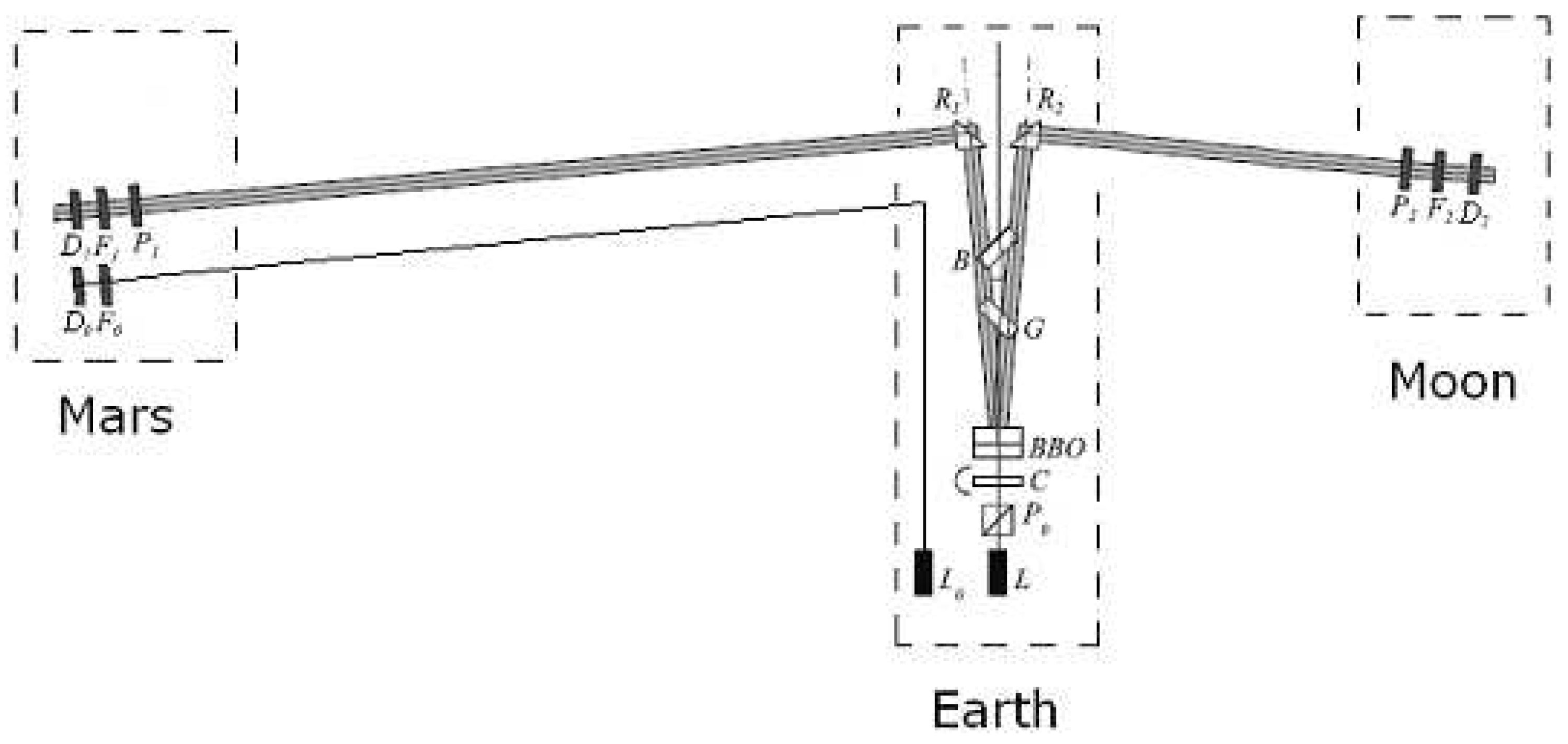
5.8. Moon-Mars measurement of photons entanglement

Since the time of wave function decay is an important factor in the measuring process, the output of quantum entanglement experiments is necessarily influenced by this factor. While it is challenging to precisely measure the time it takes for information to transfer itself via entangled photons in a laboratory, this parameter can be more accurately controlled in experiments conducted over planetary distances.

The SQHM theory aligns with the idea that relativistic causality and quantum non-locality are compatible, a concept that is already supported by relativistic quantum field theory. In order to check this, we analyze the output of two entangled photons experiment traveling in opposite direction, in the state

$$|\psi >=\frac{1}{\sqrt{2}}|H,H>+e^{i\phi }|V,V>$$

(5.62)

that cross polarizers oriented in the same direction following the scheme in Figure 1, where $H$ and $V$ are orthogonal directions of polarization.

The assumption that the state of the photon is defined only after the measurement leads to accept that the photon superposition state, interacting with the polarizer, is still not fully collapsed neither to $|H>$ nor to $|V>$until it is adsorbed or goes through the polarizer.

Given that in the SQHM approach the wave function collapse is not instantaneous but it takes a finite time interval, we name them $\Delta t_1$ and $\Delta t_2$ for the two photons, respectively.

Moreover we assume that the measurement time ${\tau }_m$ starts at the detection of the first entangled photon by the polarizer-photon counter system (at the time $t_1$) and ends when the other entangled photon is detected at the second polarizer-photon counter system (at the time $t_2=t_1+\tau {}_m$). We also assume that the detection of each photon immediately happens at the end of its wavefunction collapse.

The better way to perform the experiment is to increase as much as possible the distance $L$ between the two polarizer-photon counter systems. To comply with this requirement, we can think to have the photon source on the Earth, the first polarizer-photon counter system on the Moon and the second one on Mars.

Just for instance, we can suppose that the Moon, the Earth and the Mars are aligned each other. In this case , it follows that the distance $L$ between the two polarizer-photon counter systems reads $L=D_{e-mo}+D_{e-ma}$ and that $t_1=\frac{D_{e-mo}}{c}+\Delta t_1$, $t_2=\frac{D_{e-ma}}{c}+\Delta t_2$, where $D_{e-mo}$ and $D_{e-ma}$are the Earth-Moon and the Earth-Mars distances respectively.

Here we assume that the detection measurement follows the quantum mechanical probability. In order to determine the modality by which the quantum potential brings the information about the first photon detection to the second one, we assume that

The quantum potential interaction propagates itself at the speed of light;

The quantum potential has the spatial extension equal to the physical length${\lambda }_{qu}$ .

At the time $t=0$the first photon arrives and interact at the moon polarizer, at time $t_1=\Delta t_1$ its wavefunction decays at the final measured state, the second photon arrives on mars at $t=\frac{D_{e-ma}-D_{e-mo}}{c}$, the quantum potential signal generated by the first photon interaction (at $t=0$) reaches the second polarizer on Mars at the time

$$t=\frac{D_{e-mo}+D_{e-ma}}{c}$$

(5.63)

Besides, at the time

$$t_2=\frac{D_{e-ma}-D_{e-mo}}{c}+\Delta t_2$$

(5.64)

the second photon on mars has decayed to its final state and measured.

Thus, assuming no superluminal transmission of information it must result

$$t_2=\frac{D_{e-ma}-D_{e-mo}}{c}+\Delta t_2>\frac{D_{e-mo}+D_{e-ma}}{c}$$

(5.65)

and therefore,

$$\Delta t_2>\frac{2D_{e-mo}}{c}\cong 2.55s$$

(5.66)

where $\frac{D_{e-ma}-D_{e-mo}}{c}$has to be measured by utilizing parallel not-entangled photons.

Moreover, in order the two photons are quantum entangled, it must also hold that

$${\lambda }_{qu}>2D_{e-mo}+c\Delta t_1$$

(5.67)

The value ${\lambda }_{qu}$ of in (5.67) can be obtained by knowing the spectral composition the photon (see appendix G). In this case when the photon “one” interacts with the polarizer on the moon, it still is entangled with the photon “two” traveling toward Mars.

In this scenario, photons "one" and "two" form a single quantum system that interacts with the polarizer on the moon when photon "one" reaches it. After interacting with the polarizer on the moon, photon "two" travels to Mars carrying in its quantum potential the information about the polarization of photon "one". At this point, we essentially have an "entangled interaction" of the two photons with the first polarizer.

Equation (5.66) has been derived by assuming that the decay of photon "two" to the final measured state begins upon its arrival at the polarizer on Mars, and that the quantum potential effect, resulting from the decay of photon "one" on the moon, starts to affect photon "two" after its arrival at the polarizer on Mars (but not during its travel).

On the other hand, if

$$\Delta t_2<\frac{2D_{e-mo}}{c}\cong 2.55s$$

(5.68)

it means that the decay of the photon wave function on Mars into the polarizer-photon counter occurs before the arrival of the quantum potential interaction (information) from the first photon detection on the Moon. If the output of the measurement follows the quantum correlation law, this violates the relativistic local causality.

Furthermore, to detect the photons entangled interaction with the moon polarizer, a counter-experiment can be conducted by enclosing the Moon polarizer-detector in a Faraday cage (of about 300 meters long), with a diaphragm that closes as soon as the photon enters the cage and before it reaches the Moon polarizer. The closure of the diaphragm forces the two-photon system to interact with the macroscopic environment before interacting with the Moon polarizer. As a result, the photons should decay into decoherent states before their detection and show stochastic polarization states.

5.9. The quantum potential range of interaction of photon

Given the photon wavefunction

$$\psi ={\displaystyle \underset{}{\overset{}{\int }}{b}_k\left|{\psi }_k\right|\cos [k_{\mu }{q}^{\mu }]d^{4}k=}{\displaystyle \underset{}{\overset{}{\int }}{A}_k\cos [(kq-\omega t)]dk}$$

(5.69)

with Gaussian spectrum$A_k\propto e^{-\frac{{\left(k-k_0\right)}^2}{2\Delta k}}$ , the quantum correlation length

$${\lambda }_{qu}={\lambda }_c\frac{{\displaystyle \underset{0}{\overset{q_{\max }}{\int }}{q}^{-1}{|{\partial }_q\left(\frac{{\partial }_q{\partial }_q\left|\psi \right|}{\left|\psi \right|}\right)|}_{(r,\theta ,\phi )}dq}}{{|{\partial }_q\left(\frac{{\partial }_q{\partial }_q\left|\psi \right|}{\left|\psi \right|}\right)|}_{(q={\lambda }_c,\theta ,\phi )}}$$

(5.70)

reads (see appendix G)

$$\begin{array}{l}{\lambda }_{qu}=2{\lambda }_c\frac{{\displaystyle \underset{0}{\overset{\infty }{\int }}{x}^{-1}{|\left(-\Delta k^{4}x\right)|}_{(x,\theta ,\phi )}dx}}{{|\left(-\Delta k^{4}x\right)|}_{(x={\lambda }_c,\theta ,\phi )}}\\ =\frac{1}{2}{\displaystyle \underset{0}{\overset{\infty }{\int }}dx}=\infty \end{array}$$

(5.71)

The same result is obtained if we use the superposition of the two photons fields in calculating the quantum coherence length ${\lambda }_{qu}$.

This output allows the possibility that the two entangled photons undergo “entangled interaction” when interacting with the first polarizer on the moon generating the “synchronized decay” at the second polarizer on Mars

5.10. Extending quantum coherence to achieve a large number of entangled Q-bits

If we examine the two quantum coherence lengths, denoted as ${\lambda }_c$and${\lambda }_{qu}$, we can develop methodologies to extend quantum coherence over macroscopic distances and achieve a system comprised of a large number of Q-bits. The first proposed approach, advocated by ${\lambda }_c$, involves lowering the temperature, a method already in use but one that imposes significant constraints on the maintenance of quantum computers. A more intriguing possibility arises from analyzing ${\lambda }_{qu}$, where an expansion of the range of interaction of the quantum potential can be leveraged to increase the physical dimensions of the Q-bit system.

One initial insight gleaned from this analysis is that extending the linear range of interparticle interaction can enhance the system size at which quantum behavior remains observable. Furthermore, given that the Hamiltonian interparticle interaction becomes more robust as it strengthens, we can extend the range of quantum potential interaction by reducing the spatial dimensions of intermolecular interactions. This can be achieved through materials composed of two-dimensional structures, such as graphene, or linear one-dimensional molecules, as found in polymers. Notably, the superconducting phase of polymers may endure even at relatively high temperatures. Under the light of the stochastic quantum hydrodynamic theory, the superconducting polymers research appears to be the more promising in achieving the room temperature quantum computers. The use of linear systems for Q-bits can also gain advantage by the utilization of photon fields since ${\lambda }_{qu}$ infinite among entangled photons.

5.11. Conclusion

The stochastic quantum hydrodynamic model proposes a way to describe the behavior of quantum systems in the presence of fluctuations in the physical vacuum with a fluctuating metric. The model suggests that the spatial spectrum of noise is not white and has a correlation function with a well-defined physical length determined by the De Broglie characteristic length. This leads to effective quantum entanglement that cannot be removed in systems whose physical length is much smaller than this length.

The non-local quantum interactions may extend beyond the De Broglie length up to a distance that may be finite in non-linear weakly bonded systems.

The Langevin-Schrodinger equation can describe the dynamics of these systems, departing from the deterministic limit of quantum mechanics.

The text is discussing the relationship between the Langevin-Schrodinger equation and the physical length of a system. The equation is derived by considering the effects of fluctuations on systems whose physical length is of the order of the De Broglie length. However, as the physical length of the system increases, classical physics may be achieved when the scale of the problem is much larger than the range of interaction of the quantum potential. This is because the long-distance characteristics of the quantum potential and its range of interaction determine the existence of a coarse-grained classical large-scale description.

The SQHM also shows that the minimum uncertainty during the process of measurement asymptotically converges to the quantum uncertainty relations in the limit of zero noise. The principle of minimum uncertainty holds only if interactions and information do not travel faster than the speed of light, which is compatible with the relativistic macroscopic locality and the non-local quantum interactions at the micro-scale.

The stochastic quantum hydrodynamic model (SQHM), which suggests that the interaction of a quantum system with its environment leads to a gradual loss of coherence and the emergence of classical-like behavior, is compatible with the decoherence approach. In the SQHM, the quantum potential is not able to maintain coherence in the presence of fluctuations, due to the emergence of a drag force leading to a relaxation process known as decoherence.

This effect can be observed in macroscopic systems, such as those made up of molecules and atoms interacting by long-range weak potentials, like in the Lennard-Jones gas phase. In such systems, the effects of decoherence become more pronounced and the quantum behavior of the system becomes increasingly difficult to observe as the system size and complexity increase. The SQHM provides a useful framework for understanding the interplay between quantum mechanics and classical behavior in such systems.

The stochastic quantum hydrodynamic model suggests that classical mechanics can arise in a quantum system when the system is large enough and subjected to background fluctuations of the underlying spacetime. When a quantum system’s eigenstates are subjected to fluctuations, their stationary configurations are slightly perturbed but remain stationary and close to those of quantum mechanics.

However, when the system evolves in a superposition of states, the fluctuations cause the superposition to relax to the stationary configuration of one of the eigenstates that make up the superposition. This leads to the emergence of classical mechanics on a large scale driven both by temperature, as for the fluid-superfluid transition of${}^{4}He$, and for the extension of the quantum potential range of interaction as for the soli-fluid transition at melting point of crystal lattice. The model provides a general path-integral solution that can be obtained in recursive form. It also contains conventional quantum mechanics as the deterministic limit of the theory.

According to the stochastic quantum hydrodynamic model, decoherence is necessary for a quantum measurement to occur and that it also contributes to the execution, data collection, and management of the measuring apparatus. The model suggests that the phenomenon of wavefunction collapse in the Copenhagen interpretation of quantum mechanics may align with the concept of wavefunction decay. This decay process has its own distinct kinetics and a finite timespan associated with it. With the premise that wavefunction decay occurs within a finite timeframe during the measurement process, a thought experiment is conducted to scrutinize the measurement of photon entanglement. This experiment aims to assess whether information can propagate faster than the speed of light in the realm of quantum interactions.

The model shows that if reversible quantum mechanics is realized in a static vacuum, the measurement process cannot take a finite time to occur.

References

- Nelson, E. Derivation of the Schrödinger Equation from Newtonian Mechanics, Phys. Rev. 150, 1079 (1966).
- J. Von Neumann, Mathematical Foundations of Quantum Mechanics, translated by R. T. Beyer (Princeton University Press, Princeton, New Jersey, 1955.
- Kleinert, H. , Pelster, A., Putz, M. V., Variational perturbation theory for Marcov processes, Phys. Rev. E 65, 066128 (2002).
- Venuti, L.C. The recurrence time in quantum mechanics arXiv:1509.04352v2 [quant-ph]. arXiv:1509.04352v2 [quant-ph].
- Madelung, E.Z. , Quantentheorie in hydrodynamischer form, Phys. 1926, 40, 322–326.
- Jánossy, L. Zum hydrodynamischen Modell der Quantenmechanik. Z. Phys. 1962, 169, 79. [Google Scholar] [CrossRef]
- Birula, I.B.; Cieplak, M.; Kaminski, J. Theory of Quanta; Oxford University Press: New York, NY, USA, 1992; pp. 87–115. [Google Scholar]
- Chiarelli, P. Can fluctuating quantum states acquire the classical behavior on large scale? J. Adv. Phys. 2013, 2, 139–163. [Google Scholar]
- Chiarelli, S. , Chiarelli, P., Stochastic Quantum Hydrodynamic Model from the Dark Matter of Vacuum Fluctuations: The Langevin-Schrödinger Equation and the Large-Scale Classical Limit. Open Access Library Journal 2020, 7, e6659. [Google Scholar] [CrossRef]
- Y.B., Rumer, M.S., Ryvkin Thermodynamics, Statistical Physics, and Kinetics. Moscow: Mir Publishers; 1980; pp. 444-54.
- Ruggiero, P. and Zannetti, M., Quantum-classical crossover in critical dynamics, Phys. Rev. B 27(5), 3001 (1983).
- Ruggiero, P. and Zannetti, M., Critical Phenomena at T=0 and Stochastic Quantization Phys. Rev. Lett. 47, 1231 (1981).
- Ruggiero, P. and Zannetti, M., Microscopic derivation of the stochastic process for the quantum Brownian oscillator, Phys. Rev. A 28, 987 (1983).
- Ruggiero, P. and Zannetti, M., Phys. Rev. Lett. 48, 963 (1982).
- Chiarelli, S. and Chiarelli, P. Stability of quantum eigenstates and kinetics of wave function collapse in a fluctuating environment. arXiv 2020, arXiv:2011.13997v1. [Google Scholar]
- Bressanini, D. (2011) An Accurate and Compact Wave Function for the 4 He Dimer. EPL, 96, Article ID: 23001. [CrossRef]
- Chiarelli, P. Quantum to Classical Transition in the Stochastic Hydrodynamic Analogy: The Explanation of the Lindemann Relation and the Analogies Between the Maximum of Density at He Lambda Point and that One at Water-Ice Phase Transition. Physical Review & Research International 2013, 3, 348–366. [Google Scholar]
- Chiarelli, P. The quantum potential: the missing interaction in the density maximum of He4 at the lambda point? Am. J. Phys. Chem. 2014, 2, 122–131. [Google Scholar] [CrossRef]
- Gross, EP. Structure of a quantized vortex in boson systems. Il Nuovo Cimento,1961;20(3):454–457. [CrossRef]
- P.P.Pitaevskii,”Vortex lines in an Imperfect Bose Gas”, Soviet Physics JETP. 1961;13(2):451–454.
- Ibid [10], pp. 260.
- E.L. Andronikashvili Zh. Éksp. Teor. Fiz, Vol.16 p.780 (1946), Vol.18 p. 424 (1948).
- C.W. Gardiner, Handbook of Stochastic Method, 2 nd Edition, Springer, (1985) ISBN 3-540-61634.9, pp. 303-341.
- W. Zurek and J.P. Paz, Decoherence, chaos and the second law, arXiv:gr-qc/9402006v2 3 Feb 1994.
- Mariano, A. , Facchi, P. and Pascazio, S. Decoherence and Fluctuations in Quantum Interference Experiments. Fortschritte der Physik 2001, 49, 1033–1039. [Google Scholar] [CrossRef]
- Cerruti, N.R. , Lakshminarayan, A., Lefebvre, T.H., Tomsovic, S.: Exploring phase space localization of chaotic eigenstates via parametric variation. Phys. Rev. E 2000, 63, 016208. [Google Scholar] [CrossRef] [PubMed]
- Wang, C. , Bonifacio, P., Bingham, R., Mendonca, J., T., Detection of quantum decoherence due to spacetime fluctuations, 37th COSPAR Scientific Assembly. Held 13-, in Montréal, Canada., p.3390. 20 July.
- W. Zurek: Decoherence and the Transition from Quantum to Classical—Revisited (https://arxiv.org/pdf/quantph/0306072.pdf), Los Alamos Science Number 27 (2002).
- Lidar1 D., A. , and Whaley K. B., Decoherence-Free Subspaces and Subsystems. [CrossRef]
- Bassi, A. Gravitational decoherence. Quantum Grav. 2017, 34, 193002. [Google Scholar] [CrossRef]
- Pfister, C. , Kaniewski, J., Tomamichel, M., et al. A universal test for gravitational decoherence. Nat Commun 2016, 7, 13022. [Google Scholar] [CrossRef] [PubMed]
- Kowalsky, A.M.; Plastino, A. Decoherence, Antidecoherence and Fisher information. Entropy 2021, 23, 1035. [Google Scholar] [CrossRef] [PubMed]
- Cocciaro, B. , Faetti, S., Fronzoni, L. A lower bound for the velocity of quantum communications in the preferred frame. hysics Letters A 2011, 375, 379–384. [Google Scholar] [CrossRef]
Figure 1.
Schematic drawing of the experimental set up: laser sources, Polarizers, optical compensator, birefringent barium borate crystal, right angle prisms, interferometric filters, single photon counters,glass plate,beam splitter, see ref. [34].
Disclaimer/Publisher’s Note: The statements, opinions and data contained in all publications are solely those of the individual author(s) and contributor(s) and not of MDPI and/or the editor(s). MDPI and/or the editor(s) disclaim responsibility for any injury to people or property resulting from any ideas, methods, instructions or products referred to in the content. |
© 2023 by the author. Licensee MDPI, Basel, Switzerland. This article is an open access article distributed under the terms and conditions of the Creative Commons Attribution (CC BY) license (https://creativecommons.org/licenses/by/4.0/).
Copyright: This open access article is published under a Creative Commons CC BY 4.0 license, which permit the free download, distribution, and reuse, provided that the author and preprint are cited in any reuse.