Submitted:
25 September 2023
Posted:
28 September 2023
You are already at the latest version
Abstract
The German government's ambitious goal of achieving CO2-neutrality by 2045 has prompted a focus on improving building insulation as a vital step toward energy efficiency. However, in this process, existing radiators and boilers are often left unchanged, leading to inefficiencies due to oversized heating systems. This paper presents various approaches to reduce the required radiator inlet temperature, drawing on data from 100 multifamily buildings. The approaches include heat reserve reduction, heat power shifting, uniform radiator usage, and heat requirement analysis. These approaches collectively aim to lower flow temperatures and decrease peak heat loads, reducing energy consumption, and minimizing waste in compliance with the user comfort temperature. The findings reveal that the application of these methods can lead to substantial temperature reductions, with an average decrease of 20.82 K and 7.28 K for the highest necessary flow temperature in the provided example. Furthermore, peak load reductions of 21.07% and 13.65% were achieved, demonstrating the potential to enhance energy efficiency. While each approach can be applied individually, their synergistic implementation can highly increase the efficiency of water to x heat pumps, due to the lower required flow temperatures.
Keywords:
low-temperature ready
; low-temperature heating
; heat pump
; sustainable heating
; low-temperature radiator
1. Introduction
Due to the climate change and the recent Ukraine-Russian-War, which lead to an energy crisis, responsible consumption of energy resources is becoming increasingly important. More than 50% of all German apartments were heated with gas in 2021, mostly with central water heating systems. Although many buildings were renovated and provided with better insulation to make them more energy efficient, energy consumption dropped less than expected. The BaltBest-Project showed that the difference is partly due to operational management [1]. There is often no functioning night setback, summer shutdown and the operational management does not suit the building.
The operational management is often adjusted following residents complains. I.e., if an occupant complains about cold radiators, adjustments are made to increase the flow temperature and positively shift the heating curve. Improving the relationship between the occupants and the operating staff is part of the vise-i project, so that the user's understanding is sharpened and the technology can be operated optimally [2]. Usually, the person in charge lacks the information to examine and deal with the resident’s complaint in a professionally sound manner. The ideal operating setting for the individual building is not known. Therefore, the main goal of the operator is to satisfy the resident’s heat request, by increasing different settings which influence the boiler and pump power.
The goal of the carbon dioxide-free building stock can hardly be achieved by improving insulation, it further requires CO2-neutral heat generators. In recent years, a wide variety of heat pump systems have emerged as possible solutions. Due to the Carnot efficiency, heat pumps can be operated particularly efficiently if the temperature difference between the source and sink (the radiator) is rather small.
This necessity clashes with the current operation of boilers. While there is already a loss of efficiency when using gas boilers, the problem is exacerbated when using heat pumps, due to the decreasing coefficient of performance with increasing flow temperature. The importance of demand-oriented low flow temperature levels in combination with heat pump systems is therefore increasing strongly. Scientific projects such as Alfa [3], Beta Nord [4], Alliance [5] or BaltBest [1] showed the savings potential through good parameterization of heating systems.
In 2008, the patent "Method and device for setting the heating reserve “ was registered [6] .There they describe how to determine the power reserve of a radiator with known radiator parameters and various temperature sensors. With this information from all radiators, they can determine the power resistance of the entire heating circuit. They suggest using this information as input for optimization of the heating control.
However, Peak shaving is widely used in electrical engineering and has also been discussed for some time due heat supply. While the method was initially used in district heating networks [7] to shave heat power and reduce the flow temperature, it is becoming more and more present in the area of self-supplied residential buildings, due to the increasing use of decentralized heat pumps. Excess flow temperatures and heat loads can be reduced. Beltram et al. [8] showed an approach of heat peak shaving in smart homes. Therefore, this paper aims to combine both methods, adding further methods like power request analytics and uniform radiator usage.
2. Methods and Theoretical Background
2.1. Methods
The BaltBest project has collected measurement data from over 100 residential buildings with a temporal resolution of 110 seconds, since 2018. Data from heat meters, pumps, gas meters, heat cost allocators, etc. was retrieved. At the start of the project, the project properties were visited by the Techem GmbH, and information on building physics and system technology was collected. Therefore, characteristic data of each heat generator and radiator are available. Figure 1 shows the simplified BaltBest-Setup, which made it possible to follow the energy flow from the gas meter, over the boiler and the heat meter to the radiators in the tenants’ apartments. Overall, data was measured in 1154 apartments and 5649 rooms.
All measured data was split protected, meaning contact information and measurement data have been saved through different institutions to ensure data privacy for the participants. The measured data was saved in a PostgreSQL Database. Python with various packages such as Pandas, Psycopg2 or Seaborn for outputs. The main idea of the BaltBest project was to get a deeper insight into the heating behaviour of residents and the applied system technology in existing properties.
2.2. Theoretical Background
Heat Coast Allocators are usually used to provide consumption units, i.e., to allocate consumed heat shares to a radiator and a tenant. Therefore, the approximated radiator middle temperature and the room temperature at the radiator is measured. For the BaltBest project, temperature measurements were taken every 110 seconds.
Taking in account the airside and radiator side correction factors and, the logarithmic operating radiator excess temperature can be calculated [6] as
To estimate the operating power it’s necessary to have knowledge about the standard output , the logarithmic standard and operating excess temperature & and the radiator exponent [9]. Since radiators are installed in real apartments, they may be partially obstructed by furniture such as sofas and beds. This obstruction can result in heat accumulation, which can influence the radiator's operating behavior and measurements. The estimated output power may differ from the real output through the absence of specific information about the radiator exponent , it is assumed to be 1.3 for all radiators, following the guidance from Recknagel Chapter 2.6.4 - 1.2 [9].
2.2.1. Heat reserve reduction
Simplified, a radiator can be represented as a control volume with an incoming heat flow , an outgoing heat output and an outgoing heat flow . Figure 2 shows the flows and temperatures on a simplified radiator model.
The energy balance around the control volume is described in equation 3, were is the operating mass flow, the inlet temperature and the radiator outlet temperature.
According to equation 3 the radiator operating output power can be either changed by the inlet mass flow or by the temperature difference between the radiator inlet flow and the outlet flow temperatures. Only the input properties (inlet temperature and mass flow) are directly adjustable.
A steady output can be achieved by keeping a balance between the inlet flow temperature and the mass flow. By lowering the flow temperature, the spread between the inlet temperature and the return temperature is reduced, and at the same time the mass flow increases, by the opening radiator valve. To prevent supply gaps the operation mass flow should never become larger than the standard mass flow. Concluding the same operating power can be achieved by lower inlet flow temperatures and increasing mass flow, if the operation mass flow remains lower than the standard mass flow, Figure 3.
The state mass flow can be estimated within the given setup and eq. 3, simplifying no heat losses occur between the boiler and radiator. This assumption allows us to use the temperature measured by the heat meter as the radiator inlet temperature . Additionally, it is assumed that the radiators are of a substantial size:
If 0<<, then the necessary radiator inlet temperature , to keep the output power steady using the standard mass flow, can be calculated as:
If 0<<, the necessary radiator inlet temperature should be below the measured flow temperature at the heat meter. It's crucial to grasp that once this method is employed to determine the required inlet temperature, there is no remaining heat reserve. The following analysis is based on the thesis, that a further heating demand can be estimated using feedback from thermostats to the boiler.
Figure 4 shows the measured flow temperature in black and the necessary radiator inlet temperature in red. Each point present’s 120s. The radiators standard output power at , and °C is . The measured flow temperature (black) pulsed. However, the necessary inlet flow temperature, according to Equation 3, is significantly lower than the measured flow temperature.
2.2.2. Heat power shifting
High heat demands can result from the starting behaviour or the dynamics of smart thermostats. In existing buildings in Germany, there is typically a high thermal mass. Under the assumption that a constant room temperature can be maintained, there is little need to repeatedly reheat a building. To simplify, it is assumed that the heat power required to sustain a constant room temperature can be evenly distributed throughout the day. Figure 5a) shows the estimated heat output of a radiator, with a resolution of 110s. In this example, the radiators standard output power at , and °C is . The heat supply highly differs during the day between 0 and roughly 850 Watt, at an average outside temperature of 13 °C.
The average heat power is displayed as the red line at 332,4 Watt. Figure 5b) shows the required inlet temperature, assuming that the mass flow is equal to the design mass flow. Taking in account the average heat power and radiator temperature, the necessary constant inlet temperature is calculated using equation 5 and is represent by the red line. Due to the uniform provision heat, the necessary flow temperature drops significantly from 52 °C to 39 °C.
.
2.2.3. Uniform radiator usage
When rooms in flats are equipped with more than one radiator, heat is often just supplied by a single radiator [1]. Due to radiator oversizing, this operation is possible even at very low environment temperatures. Assuming, that heat for maintaining a constant room temperature provides at least the same comfort when transferred by several radiators, there is an unused heating surface potential. Potentially even heat supply lowers the necessary flow temperature, assuming the mass flow at each radiator is equal to the standard mass flow. With an even load the heating power of each radiator results in:
Considering Equations 3 & 5 the middle temperature at each radiator (simplified for large radiators) can be estimated as:
Due missing measurement data of the room temperatures , during the following analysis, the room temperature will be simplified as the measured air temperature at the inactive radiator. The necessary radiator inlet temperature can be calculated using equation 5, therefore it must be understood, that the radiators are supplied by the same heat circuit.
Figure 6 a) shows an example of the output power of two radiators in a single room over 24 hours. Each measuring point corresponds to 110 seconds. The radiator 5608 (blue, W) does not emit any heat, while the radiator 5609 (red, W) emits up to 1400 watts. Figure 6 b) shows the possible output power distribution according to Equation 6.
Figure 7 a) It illustrates the state excess temperature (radiator 5609 in red) and the potential excess temperatures (5608, 5609 in black) for both radiators. Since both radiators have the same standard temperatures and are operating at the same percentage of load, the required excess temperature is identical. It's important to note that this method does not account for any potential heat accumulation, although the radiator temperature may deviate from the calculated radiator temperature. Considering this, we can calculate the radiator middle temperature using Equation 7. The radiator inlet temperature, at the state mass flow, is determined using Equation 5. In Figure 7b) the necessary inlet temperature with even load (black) is up to 10 K lower than the necessary inlet temperature with uneven load (red).
2.2.4. Heat requirement analysis
The required flow temperature depends on the degree of radiator utilisation. If the radiator load is close to the standard output, no significantly lower necessary inlet temperatures are to be expected. Since users tend to use existing energy waste potential [10], it’s required to determine whether the heating power being consumed is required. Due to different usage and effects like shading or internal heat losses it’s hard to determine the required heat power to contain a constant room temperature.
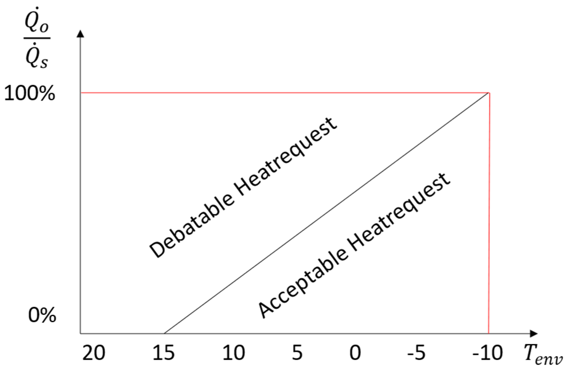
Though it should be understood, that if radiators are not undersized, they should be able to keep a steady room temperature between 15°C at the standard environment temperature (mostly -10 °C). Simplified the heat losses grow linear from the heating boundary at 15°C and 0% heat power, until the standard environment temperature at 100% heat capacity, Figure 6. If , then the requested heat power is larger than necessary to satisfy heat losses through transmission and normal ventilation behaviour but starting processes. Considering the growing over dimension of radiators, it may be necessary to undertake additional work in the future to determine the exact radiator dimensions. However, following the reduction potential is investigated, exceptionally up heating processes.
Figure 8.
Estimation of the heat request weight.
3. Results and Discussion
A property in Bad Driburg (Germany) is utilized to demonstrate the presented methods. Real measurement data collected in 2021 from heat quantity meters and corresponding heat cost allocators is used. The property has been energetically renovated in recent years and has a heated area of 700m², divided into 12 apartments, with 59 rooms and 60 radiators. The average heat transfer coefficient of the property is 0.8 W/m²K. The radiators are designed for standard operation with 70°C flow temperature, 55°C return temperature at 20°C room temperature. The design power of the radiators is between 1140W and 3712W. Average daily outdoor temperatures (red) at the site range from -14°C to about 25°C. Figure 9(a) shows that the average supply temperatures (blue) are between 35°C and 75°C. Figure 9(b) shows aggregations of the mass flow ratio in this property. The mass flow ratio is the ratio of the used mass flow in a radiator to the corresponding design mass flow. The average daily mass flow ratio (black) is at a maximum of about 11%. If you filter inactive radiators out (brown), the average is between 7% and 30%. The maximum daily mass flow ratio (red) is usually in a range below 60% and shows the highest demanding radiator of each day. There are permanently inactive radiators, so the minimum average daily mass flow ratio (blue) is 0%.
3.1. Applied Heat reserve reduction & Heat power shifting
The use of the heating reserve as shown in chapter 3.1 is applied to all radiators of the property. The necessary flow temperature, to maintain the current average radiator temperature and power output, differs greatly between radiators. In practice, the flow temperature is specified for each heating circuit, sometimes in a large heating circuit for the entire property. Thus, it is difficult to lower the flow temperature to the needs of a single radiator. To provide a satisfying output power for all radiators, the flow temperature cannot be reduced further once a radiator is supplied with the maximum heating water mass flow (the design mass flow). When the flow temperature drops, the thermostatic valves of the radiators open. They try to compensate for the resulting loss of power by increasing the mass flow. It is important to determine the point at which the first radiator valve is completely open. The limit flow temperature (red) and the measured flow temperature (blue) are shown in Figure 10 a). The limit flow temperature (highest necessary flow temperature) already provides a potential to lower down the flow temperature, compared to the measured flow temperature. The median of the required flow temperature (not considering the inactive radiators; brown) is between 30 and 40 °C. Figure 10b) shows the difference between the measured flow temperature and the limit flow temperature (red) and median necessary flow temperature (brown).
Notice, the median and limit flow temperature differ a lot. Simply applying the reserve reduction and heat power shifting alone does not lead to a noticeable reduction of the necessary flow temperature in all cases. Through the conception of water heating systems, the highest necessary flow temperature for a single radiator must be supplied to the whole heat circle.
Like shown in Figure 3 the method of heat reserve reduction can be applied if 0<<. Excluding the summer months (May till September) and inactive radiators, the flow temperature could be decreased by 20,82 K on average over all radiators in 2022. Considering the limiting highly used radiators, the flow temperature could be decreased by 7,28 K on average. That shows the negative impact of the highly used radiators.
3.2. Applied uniform radiator usage
In our example, there is one room with two radiators. Radiator 1 has a design power of 2.911 W, radiator 2 has 2.079 W. Contrarily to the size of both radiators, radiator 1 emitted a total heat energy of 1284 kWh and radiator 2 a total of 1732 kWh, Figure 12 a. The respective full load time of radiator 1 is at 390 h and radiator 2 is at 716 h. By using equation 6 the heat load is evenly distributed, weighted by their design power, resulting in 525 h full load time for each radiator.
The calculation was carried out in time steps of five minutes, so that peak loads could still be evaluated. The inner temperature was calculated according to equation 7 and the new inlet temperature according to equation 5. For each time step, the maximum necessary temperature (from one of the two radiators) was taken to ensure proper heat supply. These values were averaged over the whole heating period. The necessary inlet temperature reduced from 39.0 °C to 32.6 °C for this room, see Figure 12 b.
3.3. Applied Heat Requirement analysis
The heat requirement analysis from chapter 3.4 is applied to the example building.
The relative heat load is calculated for each radiator based on the average values of one hour. This time interval helps to smooth out peak values, ensuring that each data point represents a meaningful amount of energy transferred into the room. Data where the radiator was shut down has been filtered out.
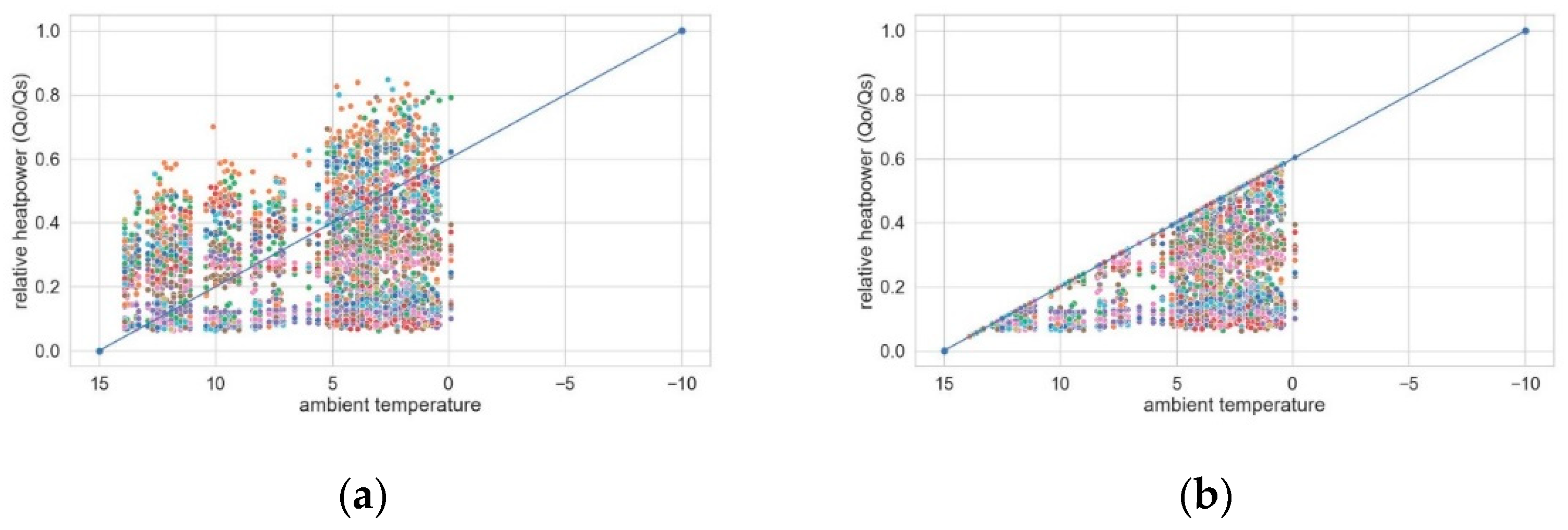
Figure 13 shows a scatterplot of all operating states over the ambient temperature from 2022-01-01 to 2022-01-10. The ambient temperature ranged from ~ 0 °C to 14 °C. The blue line represents the estimation of heat requirement. Many data points lie above the given heat requirement, which indicates an oversupply of heat. Each color represents one radiator, which allows drawbacks on individual heating behavior. For example, the orange radiator is consistently used at high power, which indicates a) waste of heat (f.e. open windows), b) excessive temperatures or c) uneven heat distribution as in chapter 3.3 (one radiator is doing all the work). Limiting the heat supply to the estimated required value, would reduce the heat load drastically, Figure 13 b.
The calculation as shown in Figure 13 b is carried out for the whole January 2022. If each state above the line is considered a waste of energy, the average load and energy consumption decreases by 13.65 %. However, even if the energy transferred into the room during each state is necessary to guarantee the comfort level, the reduction of power could be compensated by longer periods of heating, as shown in chapter 3.2. Still, peak loads can be decreased by 21.07 % and thus decreasing the necessary flow temperature.
4. Conclusions
The main objective of this study is to reduce flow temperatures and peak heat loads to facilitate the widespread integration of heat pumps, resulting in reduced energy consumption and minimized waste potential. The research introduces four distinct methods designed to achieve lower flow temperatures and heat loads within buildings without compromising room temperatures. No impact on occupant comfort is expected with any of the methods studied. However, the reduction in temperature levels and associated increase in energy efficiency may motivate occupants to address energy use and settings and provide qualified feedback for building operations.
The primary approach centers on reducing heat reserves. This involves lowering the required flow temperature by increasing the volume flow, thereby maintaining a consistent heat power output. The application of this method resulted in an average temperature decrease of 20.82 K and 7.28 K for the highest required flow temperature in the provided example, and an average decrease of 19.42 K and 9.72 K for the highest required flow temperature across 81 buildings. Another technique involves redistributing heat power to address peak loads, necessitating prolonged heating periods with reduced power. Effective management with this method may require the incorporation of more sophisticated thermostats as today's modern and intelligent thermostats tend to focus on providing heat when needed, rather than in advance. In Addition, the method of uniformly utilizing radiators aims to optimize existing potential and heat distribution, potentially significantly reducing the flow temperature when multiple radiators are available. The final method, heat requirement analysis, evaluates the appropriate heat powers for each radiator, comparing them against the current configuration. This approach proves effective when combined with heat power shifting, as it identifies peak loads and calculates suitable heat power levels. Peak load reductions of 21.07% and 13.65% were calculated in the example, while reductions of 28.52% for peak loads and 13.37% on average were calculated for all buildings.
While each method can function independently, their synergistic application can yield even greater benefits. It's important to note that the reported values are based on optimal configurations. In real-world scenarios, various factors such as hydraulic considerations, heat losses, and user interventions must be considered. This necessitates the use of a buffer to ensure a reliable heat supply.
The potential for implementing these methods exists across a wide range of buildings. A prudent initial approach involves targeting buildings already suitable for heat pump integration and subsequently optimizing their systems.
In summary, the core findings of this study emphasize a range of strategies to reduce flow temperatures and manage peak loads, ultimately enhancing energy efficiency in buildings. These outcomes underscore the feasibility of these methodologies, especially when tailored to specific contexts. By implementing these strategies and addressing practical challenges, stakeholders can embark on a path towards greener and more sustainable energy use.
Funding
This work was partly funded by the Ministry of Economic Affairs, Innovation, Digitalisation and Energy of the State of North Rhine-Westphalia (MWIDE) within the project “Smart User Interfaces – VISE-I" (grant no. EFO/0150C).
Data Availability Statement
Not available due to data privacy
Conflicts of Interest
The authors declare no conflict of interest. The funders had no role in the design of the study; in the collection, analyses, or interpretation of data; in the writing of the manuscript; or in the decision to publish the results.
References
- Grinewitschus, V.; Jurkschat, S.; Lepper, K.; Beblek, A.; Fransen, K. BaltBest: Einfluss der Betriebsführung auf die Effizienz von Heizungsaltanlagen im Bestand, 2021. Available online: https://www.ebz-business-school.de/forschung/forschungsprojekte/baltbest.html (accessed on 5 March 2023).
- Tochtrop, C. VISE-I: Smart User Interfaces. Virtuelles Institut Smart Energy (VISE) - Intelligente Bedienungsoberflächen für Nutzer*innen im energieeffizienten Haushalt [Online], September 25, 2023. Available online: https://smart-energy-nrw.web.th-koeln.de/vise-i-smart-user-interfaces/ (accessed on 25 September 2023).
- Gusek, A.; Bär, Y. ALFA®-Allianz für Anlagenenergieeffizienz: Wirtschaftlich - Sozial verträglich - Ökologisch effizient, Berlin, 2016.
- Bernd, U.; Sankol, Günter Wolter, Jörg Heermann. Betriebs Effizienz Technischer Anlagen: BETA Nord. Available online: https://www.vnw.de/interessenvertretung/technik-und-energie/beta-nord/ (accessed on 25 September 2023).
- Grinewitschus, V.; Lepper, K. Allianz: Allianz für einen klimaneutralen Wohngebäudebestand. Available online: https://www.energieeffizient-wohnen.de/ (accessed on 25 September 2023).
- Kähler, A.; Schulz, H.-J. Method and device for adjusting the heating power reserve, September 25, 2023.
- Guelpa, E.; Barbero, G.; Sciacovelli, A.; Verda, V. Peak-shaving in district heating systems through optimal management of the thermal request of buildings. Energy 2017, 137, 706–714. [Google Scholar] [CrossRef]
- Beltram, L.; Christensen, M.H.; Li, R. Demonstration of heating demand peak shaving in smart homes. Journal of Physics Conference Series 2019, 1343, 12055. [Google Scholar] [CrossRef]
- Taschenbuch für Heizung und Klimatechnik: Einschließlich Trinkwasser- und Kältetechnik sowie Energiekonzepte; Sprenger, E. ; Albers, K.-J., Eds., 78. Auflage, 2017/2018; DIV Deutscher Industrieverlag GmbH: München, 2017; ISBN 3835672843. [Google Scholar]
- Grinewitschus, V.; Jurkschat, S. BaltBest. Available online: https://www.energieeffizient-wohnen.de/baltbest (accessed on 3 November 2022).
Figure 1.
Simplified setup of the heating system and the measurement infrastructure. a) Boiler, b) Pump, c) Heat flow meter, d) Thermostat valve and e) Heat cost allocator.
Figure 1.
Simplified setup of the heating system and the measurement infrastructure. a) Boiler, b) Pump, c) Heat flow meter, d) Thermostat valve and e) Heat cost allocator.
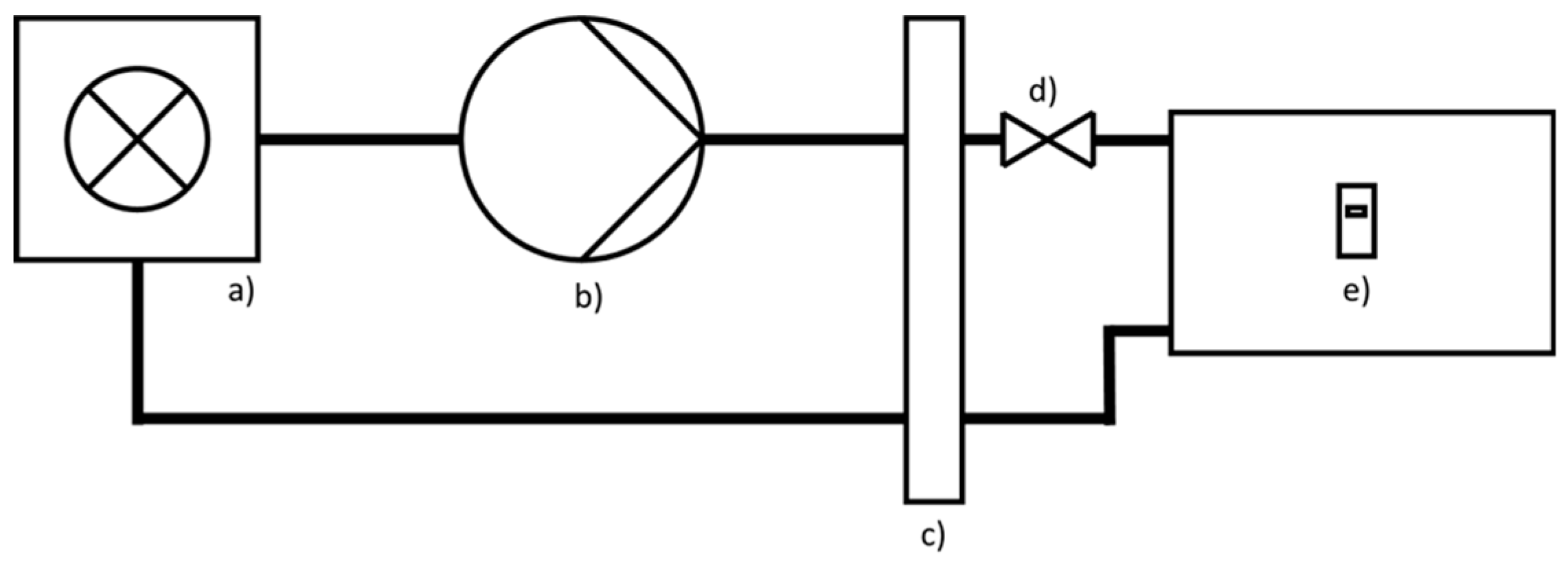
Figure 2.
Simplified radiator model with relevant input and output heat flows.
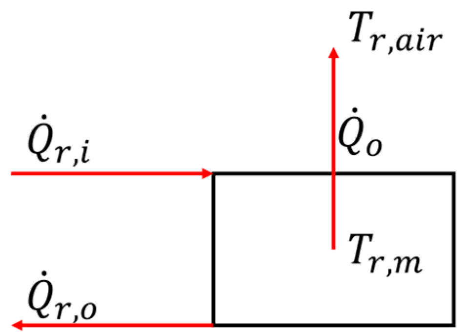
Figure 3.
Display of the state shift from s1 to s0.
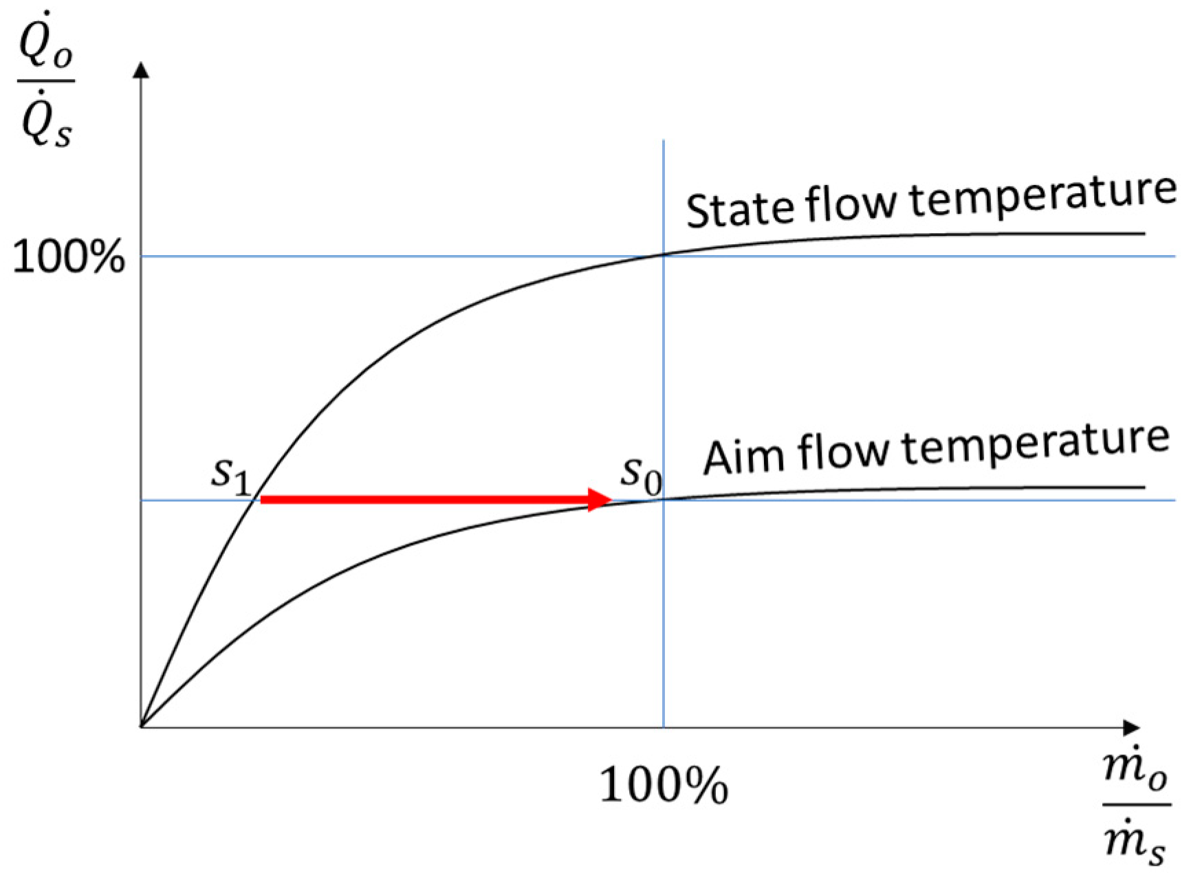
Figure 4.
Measured flow temperature (black) vs necessary flow temperature (red) at
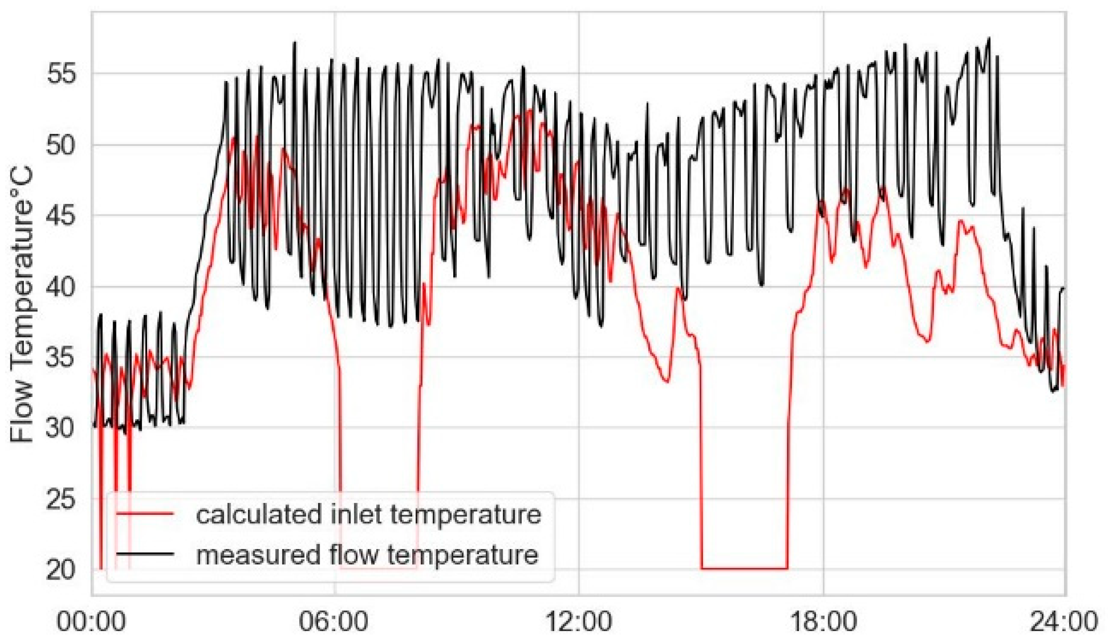
Figure 5.
Demonstration of the effect of uniform heat supply: (a) Heat supply; (b) Necessary inlet temperature at
Figure 5.
Demonstration of the effect of uniform heat supply: (a) Heat supply; (b) Necessary inlet temperature at
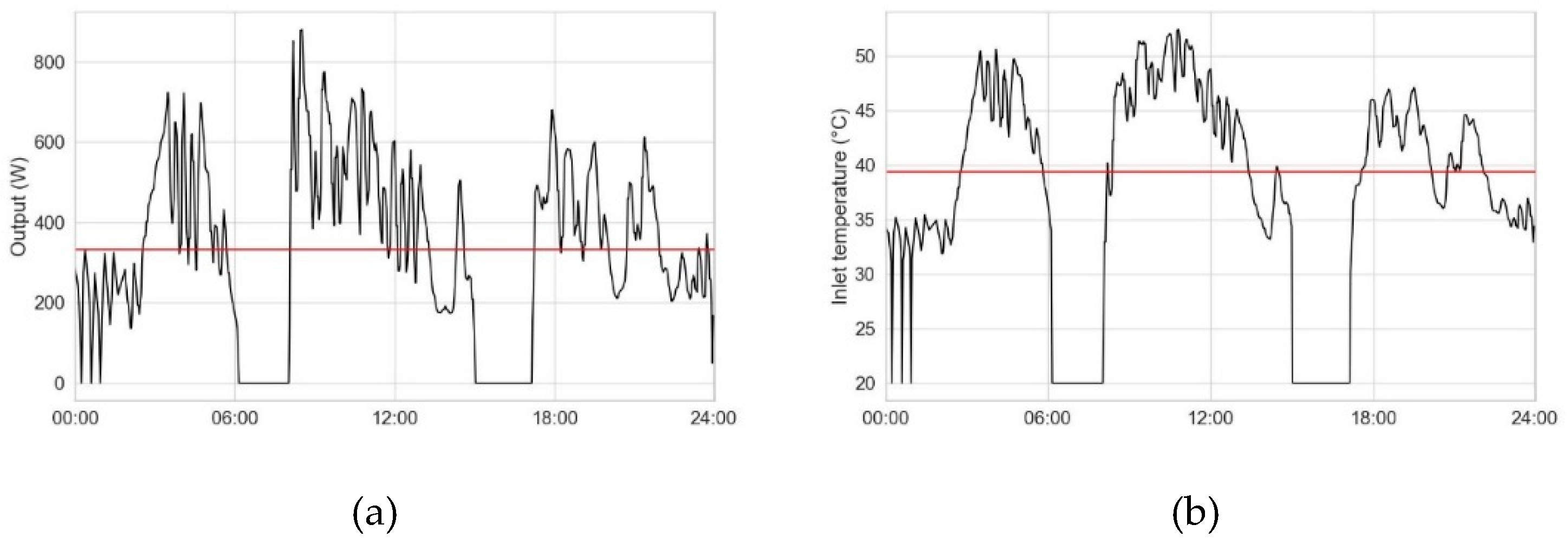
Figure 6.
Heat power distribution in an example room: (a) Measured power output; (b) Calculated power distribution for two active radiators.
Figure 6.
Heat power distribution in an example room: (a) Measured power output; (b) Calculated power distribution for two active radiators.
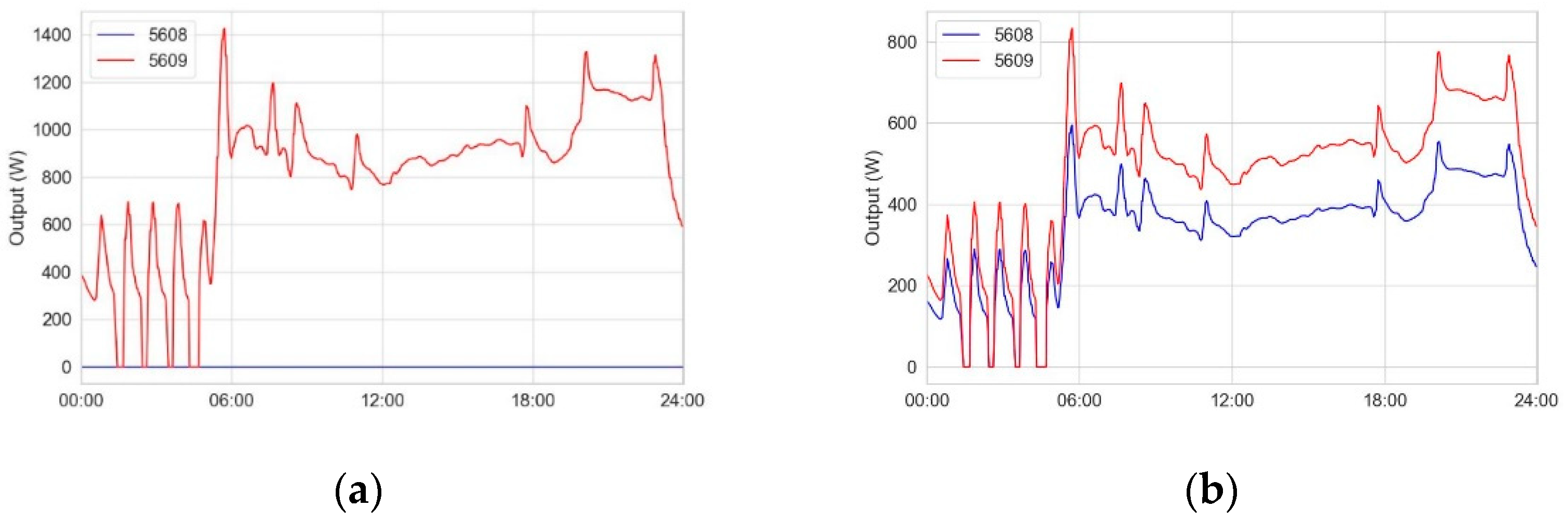
Figure 7.
Effect of load sharing on: (a) The excess temperatures; (b) The inlet temperatures.
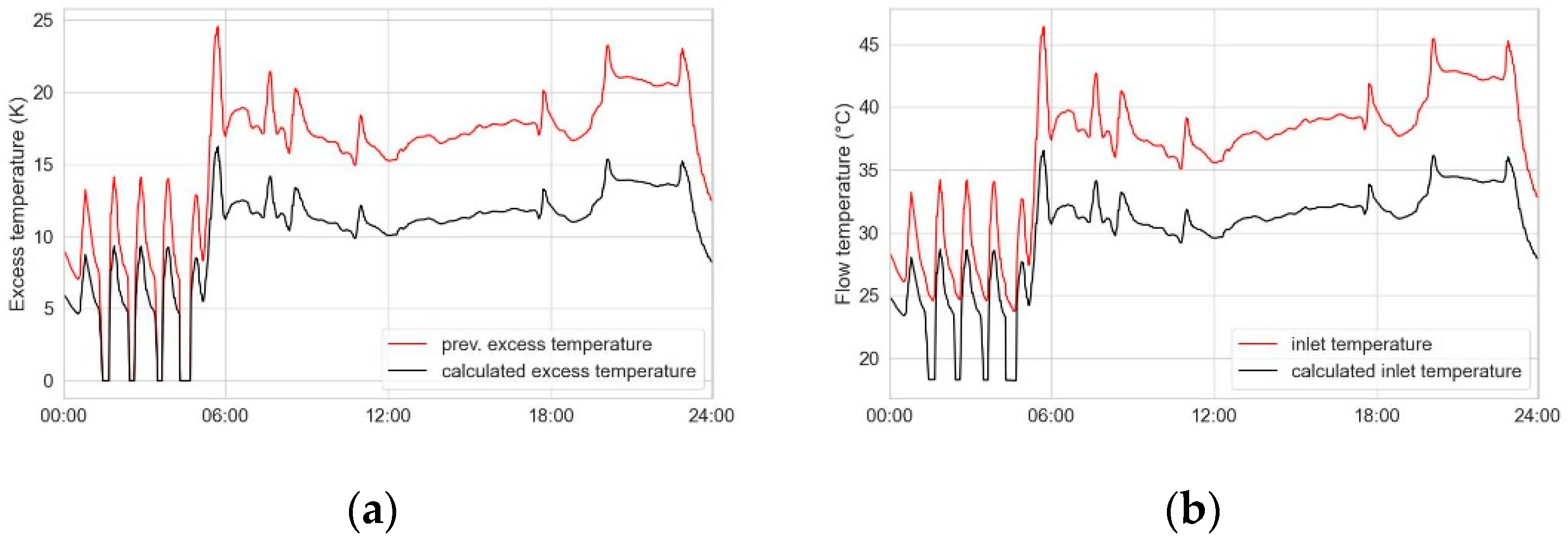
Figure 9.
(a) Daily outdoor and flow temperatures; (b) Daily mass flow ratios.
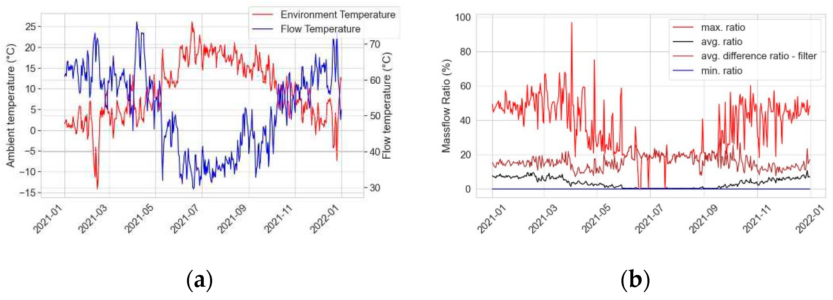
Figure 10.
Applied head reserve reduction & power shifting: (a) Flow temperatures, measured vs necessary; (b) Reduction potential.
Figure 10.
Applied head reserve reduction & power shifting: (a) Flow temperatures, measured vs necessary; (b) Reduction potential.
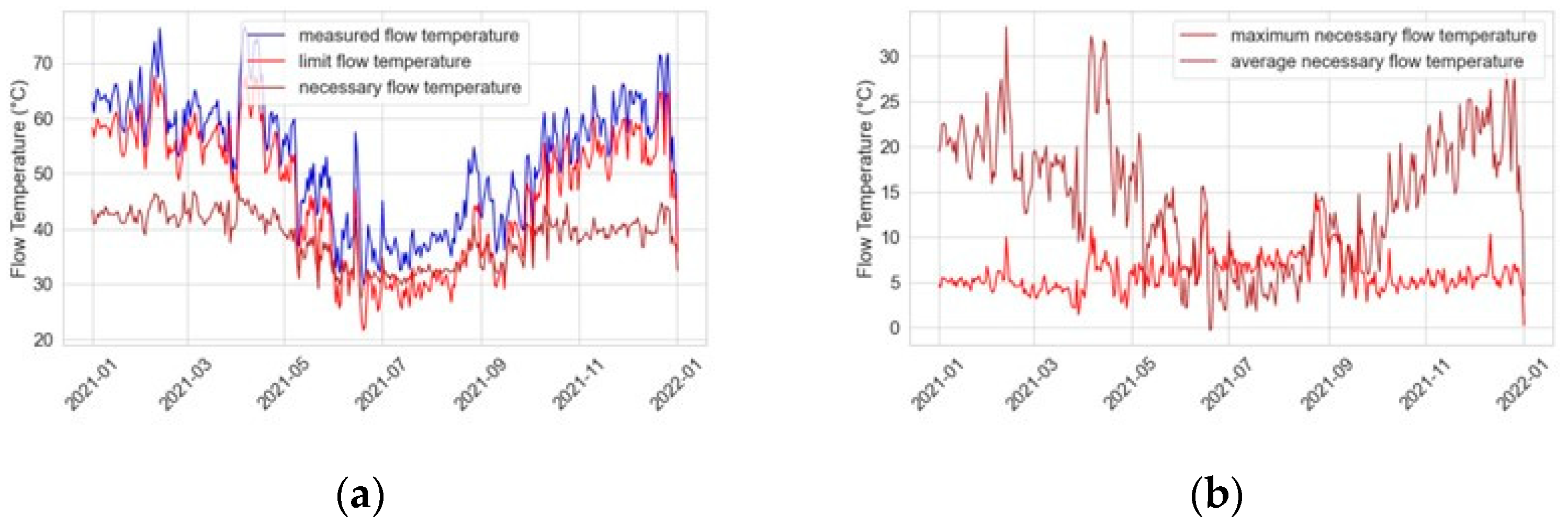
Figure 12.
Impact of applied uniform heat loads: (a) Heat distribution; (b) Potential to reduce the flow temperature for both radiators.
Figure 12.
Impact of applied uniform heat loads: (a) Heat distribution; (b) Potential to reduce the flow temperature for both radiators.
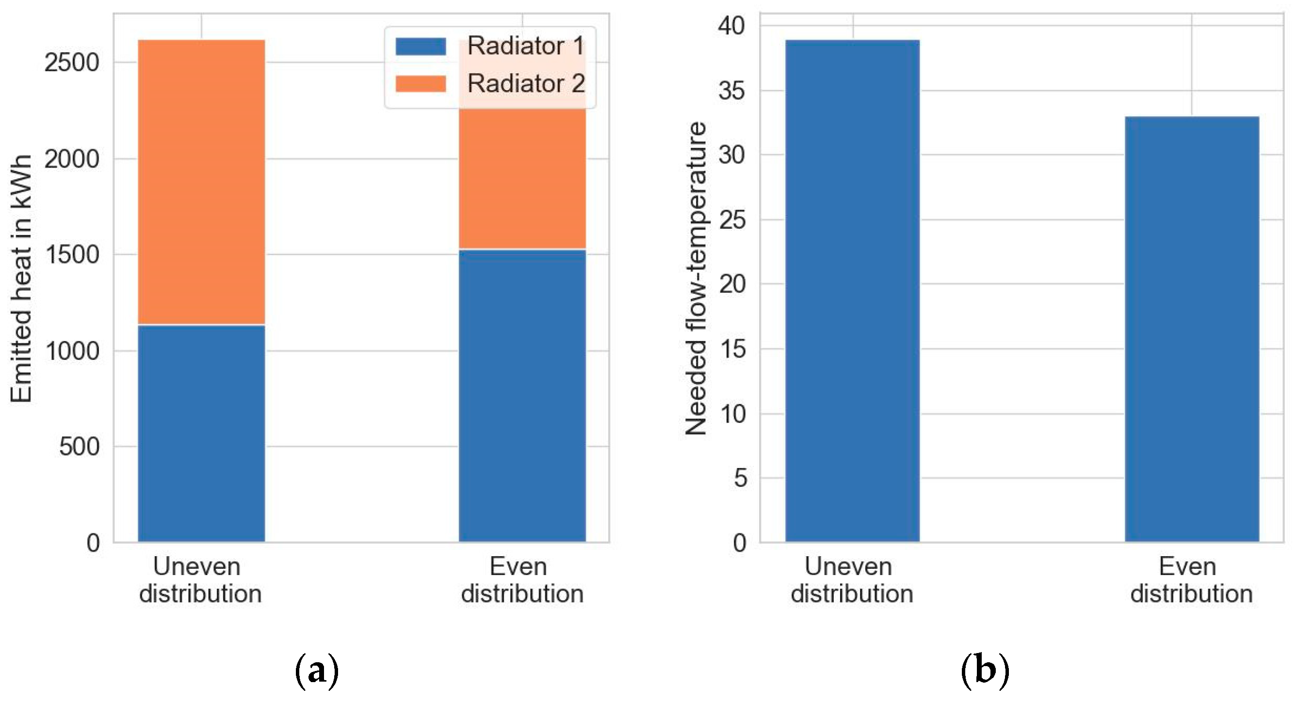
Figure 13.
Applied heat requirement analysis: (a) Operating states of radiators in the apartment building; (b) Operating states limited at the estimated heat requirement.
Figure 13.
Applied heat requirement analysis: (a) Operating states of radiators in the apartment building; (b) Operating states limited at the estimated heat requirement.
Disclaimer/Publisher’s Note: The statements, opinions and data contained in all publications are solely those of the individual author(s) and contributor(s) and not of MDPI and/or the editor(s). MDPI and/or the editor(s) disclaim responsibility for any injury to people or property resulting from any ideas, methods, instructions or products referred to in the content. |
© 2023 by the authors. Licensee MDPI, Basel, Switzerland. This article is an open access article distributed under the terms and conditions of the Creative Commons Attribution (CC BY) license (http://creativecommons.org/licenses/by/4.0/).
Copyright: This open access article is published under a Creative Commons CC BY 4.0 license, which permit the free download, distribution, and reuse, provided that the author and preprint are cited in any reuse.


