
Submitted:
25 September 2023
Posted:
25 September 2023
You are already at the latest version
Abstract
Sea cucumber detection represents a significate step in underwater environmental perception, which is an indispensable part of the intelligent subsea fishing system. However, various complex factors such as water turbidity declines the clarity of underwater images, presenting a challenge to vision-based underwater target detection. Therefore, accurate, real-time and lightweight detection models are required. First of all, the development of subsea target detection is summarized in this presented work. Besides, since target detection methods based on deep learning such as YOLOv5 and DETR, which are respectively examples of one-stage and anchor-free deep leaning methods, have been increasingly applied in underwater detection scenarios. Based on the analysis of state-of-the-art underwater sea cucumber detection approaches and aiming to provide a reference for practical subsea identification, the sea cucumber detection based on the YOLOv5 and DETR are investigated and compared in detail. For each approach, the detection experiment is carried out on the derived dataset which contains a wide variety of sea cucumber sample images. The compared experiments demonstrate that the overall outperformance of YOLOv5 in terms of low computing consumption and high precision, particularly in detection of small and dense features. Nevertheless, the DETR exhibits rapid development and holds promising prospects in underwater object detection applications, owing to its relatively simple architecture and ingenious attention mechanism.
Keywords:
underwater target detection and recognition
; YOLOv5
; DETR
; sea cucumber fishing
1. Introduction
In recent years, with the development of automatic intelligent aquaculture and fishing technology and the improvement of human being’s living standards, the demand of aquatic products is increasing gradually, such as sea cucumbers, with high nutritional value, memory enhancing and anti-tumor effects. The sea cucumber aquaculture industry has become a major industry in certain coastal areas, bringing an increase to the income of fishermen and also promoting the development of secondary and tertiary industries, such as processing and transportation. However, there are various problems that make the fishing of sea cucumbers troublesome. Sea cucumbers have only two dormant periods in a year, thus the fishing operations can only be in spring and autumn. Additionally, due to the presence of abundant reefs in the living environment of sea cucumbers, it is unsuitable to use fishing nets for their capture. The fishing operations of sea cucumbers in most marine pastures are conducted by professional staff, who are supposed to put on oxygen masks and dive into the seabed. This traditional method of artificial fishing requires high levels of skills and takes the risk of causing various occupational diseases, due to the low temperatures of seawater in spring and autumn, the frequent changes of water pressure during diving and surfacing, and the complex seabed working environment. Therefore, replacing manual work with intelligent underwater robots which can capture sea cucumber automatically has become the development trend [1].
Perceiving the underwater environment is an integral part of the intelligent underwater fishing robot system such as Remotely Operated Vehicles (ROVs) and Autonomous Underwater Vehicles (AUVs) [2]. The system perceives information of underwater environment through acoustic or optical sensors, and then takes corresponding actions based on the surrounding area. Therefore, autonomous underwater sea cucumbers detection is a necessary step for subsea robots to localize and capture sea cucumbers automatically. High imaging resolution and rich information makes the underwater optical imaging the most intuitive and commonly used method for information acquisition. However, the turbidity and poor light transmittance of water cause a significant reduction in the clarity of underwater images, presenting a challenge to the practice of vision-based underwater target detection [3]. Turbidity is often encountered in sea cucumbers’ complex living environment. The direction of light transmission is affected by the scattering or absorption of water and various organic and inorganic suspended particles such as fishes and sediments, which leads to image distortion, such as blurred target features, severe distortion, and color changes. Besides, the low light conditions result in receiving limited effective target light information. Thus, current researches on underwater vision are mainly focusing on scenarios with good water conditions. Moreover, marine creatures such as sea cucumbers are usually small in size, making it difficult to detect and recognize. Therefore, the research of object detection and recognition in complex and changeable underwater areas is challenging but essential.
The target detection in underwater areas need to consider image restoration and enhancement. Compared with that in atmospheric environment, mainly the traditional detection approaches and deep learning-based methods are taken into account. In the classic methods, the interest regions are firstly selected through sliding windows, and features within them are extracted through conventional algorithms including Scale Invariant Feature Transform (SIFT) [4], Histograms of Oriented Gradients (HOG) [5], etc. Then, machine learning algorithms such as Support Vector Machine (SVM) [6] are applied to classify the extracted features and determine whether this region contains targets. Deep learning-based approaches study image sets by training neural networks and establish logical relationships to improve the image clarity and extract target features for intelligent recognition. Other methods for underwater target detection are also studied, including sonar imaging, laser imaging, polarization imaging, etc.
The main contributions of this presented work are summarized as follows:
- First of all, the state-of-the-art underwater sea cucumber detection approaches are summarized, including traditional methods, one-stage methods based on deep learning such as You Only Look Once (YOLO) series algorithms and Single Shot MultiBox Detector (SSD), two-stage methods based on deep learning such as R-CNN series algorithms, anchor free approaches such as DEtection TRansformer (DETR) and other methods.
- For the detection of sea cucumbers, fundamentals of YOLOv5 and DETR are firstly introduced. Then the training process, test results of YOLOv5 and DETR and the performance comparation of these two approaches are presented, proving the excellent performance of YOLOv5 and DETR in underwater sea cucumber detection.
In this manuscript, relevant research methods and the latest achievements about underwater target detection are systematically collated, and then experiments based on YOLO and DETR are carried out based on the derived sea cucumbers datasets. The rest of the manuscript is organized as follows: Section 2 briefly describes the research related to underwater target detection and the recent developments; The detection of sea cucumbers based on YOLOv5 are introduced in Section 3; Section 4 demonstrates the detection of sea cucumbers based on DETR and the performance comparation of YOLO and DETR; Finally, in Section 5, conclusions are drawn, and current problems are discussed to provide a reference for future work.
2. Related Works
With the development of underwater image processing and target detection techniques, many conventional algorithms and frameworks have been developed. Traditional target detection methods extract the features of target areas manually, which is time consuming and has poor robustness. The candidate regions are firstly selected through different sizes of sliding windows. And then features in these windows are extracted. Finally, machine learning algorithms are applied for recognition. The classic algorithms such as HOG and Deformable Part Model (DPM) [7] have some limitations. The region selection strategy is not targeted, which leads to high time complexity and window redundancy. Additionally, artificially designed methods are not as robust in terms of feature diversity as required.
With the emergence of the deep learning convolution neural network, great breakthroughs have been made in object detection algorithms. Methods based on deep learning outperform those traditional methods which demand manual intervention, thus are more suitable to deploy on underwater robots. Existing target detection algorithms are mainly divided into two categories: region proposal-based target detection algorithms, also known as two-stage algorithms, and regression-based target detection algorithms, also referred to as one-stage algorithms [8]. Two-stage ones first extract the proposed regions from the images, and then classify and regress them to obtain the detection result, mainly including the algorithms based on Region Convolutional Neural Network (RCNN) [9], Fast RCNN [10] and Faster RCNN [11]. And there are other two-stage networks that have been improved based on the above algorithms, such as Region-based Fully Convolutional Networks (R-FCN) [12], Mask R-CNN [13], and Cascade R-CNN [14]. Two-stage algorithms can obtain more accurate detection results, but the processing time increases accordingly. Single-stage algorithms improve the detection speed by detecting and localizing the targets directly from the whole image. Main representatives of single-stage algorithms are SSD [15] algorithm and YOLO algorithms (YOLO [16], YOLOv2 [17], YOLOv3 [18], YOLOv4 [19], YOLOv5 [20]). With continuous improvements and innovations, the current single-stage target detection algorithms can take the accuracy of detection into account and also guarantee speed.
Deep learning-based approaches show excellent performance, but also has some limitations, since the accuracy of detection is affected by the image quality, and deep learning methods are only applicable in waters similar to the training set image. Therefore, it is necessary to combine good image restoration methods and deep learning algorithms to make underwater target detection more effective. Thomas et al. [21] created a fully connected convolution neural network for underwater image defogging. By using the depth frame of the encoder-decoder to integrate low and high-level features, the network was able to effectively restore blurred imageries. A method of recovered images was proposed by Martin et al. [22], which combined image enhancement, image recovery, and the convolutional neural network. To address the issue of the maximum number of green pixels in underwater images, they proposed Under Dark Channel Prior method (UDCP)-based Energy Transmission Restoration (UD-ETR) method to process green channel images and obtain the recovered images. The Sample-Weighted Hyper Network (SWIPENet) was proposed by Chen et al. in 2020 [23] to cope with the blurring of underwater images in the context of severe noise interference, the architecture of which includes many semantic rich and high-resolution hyper feature maps inspired by Deconvolutional Single Shot Detector (DSSD) [24]. In [25], Dana et al. introduced an innovative approach for enhancing the colors of single underwater images. They employed a physical image formation model, distinguishing themselves from previous research. Various Jerlov water types were used to estimate transmission values through a haze-lines model. Finally, color corrections were applied using the same physical image formation model, and the optimal outcome was selected from the different water types considered.
Weibiao Qiao et al. [26] introduced a novel approach for the real-time and precise classification of underwater targets in 2021. They employed Local Wavelet Acoustic Patterns (LWAP) in conjunction with Multi-layer Perceptron (MLP) neural networks to tackle the challenges associated with underwater passive target classification, addressing issues related to heterogeneity and classification difficulty. A lightweight deep neural network was introduced in [27], aiming to simultaneously learn color conversion and object detection from underwater images. To mitigate color distortion, an initial step involves employing an image color conversion module to transform color images into grayscale ones. Subsequently, object detection is carried out on the converted grayscale images. This joint learning process involves optimizing a combined loss function. Xuelong Hu et al. incorporated PANet into Feature Pyramid Networks (FPN) [28] in [29], augmenting it to produce a diverse multi-scale feature architecture. This enhanced feature structure was subsequently employed in an uneaten feed pellet detection model tailored for aquaculture applications. Experiments demonstrate a substantial increase in Mean Average Precision (mAP) by 27.21% when compared to the baseline YOLO-v4 method [30]. To address the challenge of a constrained dataset, Lingcai Zeng et al. [31] introduced an innovative approach by incorporating an Adversarial Occlusion Network (AON) into the conventional Faster R-CNN detection algorithm. This methodology proved effective in augmenting the training data and enhancing the detection capabilities of the network. Taking inspiration from the shortcut connections observed in residual neural networks [32], Fang Peng et al. introduced a novel approach, the Shortcut Feature Pyramid Network (S-FPN) in [33]. The primary aim of which is to enhance an existing strategy for multi-scale feature fusion, particularly for holothurian detection.
Through the exploration of enhancement strategies for simulated overlapping, occlusion, and blurred objects, Weihong Lin et al. devised a practical generalized model in [34], aimed at addressing challenges related to overlapping, occlusion, and blurring of underwater targets. The Super-Resolution Convolutional Neural Network (SRCNN) is a super-resolution technique that relies on pure convolutional layers [35]. In the context of underwater imaging in low-light conditions, SRCNN has been utilized to enhance the quality of captured images [36]. To derive the low-resolution components, the raw data underwent iterative processing involving total variation regularization [37]. A method based on YOLO was introduced in [38], aimed to safeguard rare and endangered species or eradicate invasive exotic species. It was designed to effectively classify objects and count their quantities in consecutive underwater video frames. This involved aggregating object classification outcomes from preceding frames to the current frame. In [39], Minghua Zhang et al. introduced a Multi-scale Attentional Feature Fusion Module (AFFM) designed to blend semantic and scale-inconsistent features across various convolution layers. In [40,41], an innovate method merging multi-scale features across different channels was introduced, which is achieved through various kernel sizes or intricate connections within a single block. This approach enhances the neural network's capacity for representational learning by emphasizing multi-scale feature fusion within a single block, as opposed to feature fusion across multiple stages of the backbone network.
Other methods for underwater target detection are also explored, such as sonar imaging, laser imaging, polarization imaging, electronic communications, etc. In forward-looking sonar imaging, the geometry, grayscale, and statistical features of some interferences are similar to that of the targets, which leads to difficulty for targets detection. Thus, an underwater linear target detection technology was proposed by Liu [42], combining the Hough transform and threshold segmentation, which can effectively extract linear objects. The research in [43] introduces a tracking filter designed to combine Ultrashort-base Line (USBL) measurements and acoustic image measurements. This approach could achieve dependable underwater target tracking.
2.1. Dataset and Evaluation Metrics
The deep learning-based underwater sea cucumber detection requires a large number of images for training. The experimental dataset of sea cucumbers is provided by Shandong Future Robot Co., Ltd [44], which contains a wide variety of sea cucumbers’ sample images. The targets in the dataset are labeled and images which do not contain the detected targets are removed. 3271 valid images are retained after pre-processing, the resolution of which is 416x416 pixels. With a total of more than 10,000 ground truth data for training, all images are processed and stored according to the PASAL VOC dataset format.
One of the key points to the underwater detection is the diversity of the underwater environments contained in the dataset as well as the variety of target poses and density. This dataset includes sea cucumber images under different conditions, for instance, above water surface, in the clear underwater area, in the turbid underwater area, in the accumulation area and the sparse area of sea cucumbers. Examples of sample images are depicted in Figure 1, which clearly demonstrate the problems faced in underwater detection: the turbidity of subsea area and multi-object occlusion in the accumulation area. Multiple types of samples improve the robustness of the model and enable it with strong adaptability to various special cases. In addition, the performance comparison of sea cucumber detection by the YOLOv5 and DETR approach will be conducted based on these unique types of sample images.
The computer configuration is also a crucial factor affecting the model training and detection results. The training and performance comparison of the YOLOv5 and DETR model for sea cucumber detection are carried out under the experimental environment configurations listed in Table 1.
For the performance evaluation and comparation of target detection, the definitions of performance evaluation indicators need to be clarified. Precision and recall are the most widely used evaluation metrics, which are computed based on the confusion matrix, as described in Equations (1) and (2):
where TP, FP, and FN denote ’True Positive’, ’False Positive’, and ’False Negative’, respectively. They are defined according to the Intersection over Union (IoU) between the predicted bounding box and the ground truth. If the IoU is greater than the threshold, the bounding box is marked as TP, representing the number of correctly identified targets, otherwise it is labelled as FP, implying the number of incorrectly identified targets.
Precision and recall are correlative. For the model with better performance, its precision keeps high while the recall rate increases. Thus, by combining these two indicators, Average Precision (AP) and the mean AP of all categories (mAP) are defined, which are calculated by Equations (3) and (4). In addition, the F1 score shown in Equation (5) is another commonly used metric for evaluating binary classification problems, which is the harmonic average of precision and recall mentioned above.
where P, R and C refers to precision, recall and the number of target categories individually. The value of AP is also equal to the area under the precision-recall curve. mAP@0.5 denotes the mAP value calculated when the threshold of the IoU is 0.5. mAP@0.5:0.95 refers to the average value from mAP@0.5 to mAP@0.95 (mAP@0.5, mAP@0.55, ..., mAP@0.9, mAP@0.95). The higher the AP or mAP value is, the higher the accuracy of the model achieves.
3. Yolov5
3.1. Fundamentals of YOLOv5
a. Model Structure
YOLOv5 was proposed by Glenn Jocher in 2020 [20], outperforming the previous YOLO series algorithms in terms of flexibility and speed, and showing its strong advantage in rapid deployment of the model. YOLO series algorithms are typical representatives of the one-stage methods, also referred to as regression-based target detection algorithms. The central concept of YOLOv5 remains the same as previous versions, which is to divide images into regions firstly and predict bounding boxes and probabilities for each area. The results are then refined based on anchor boxes and Non-Maximum Suppression (NMS) is used to remove overlapping detections. There are four versions of YOLOv5: YOLOv5x, YOLO5l, YOLO5m and YOLO5s, different in depth and width, of which YOLOv5s is the smallest in network depth and width. YOLOv5 mainly consists of four parts: the input module, the backbone network for feature extraction, the neck network for feature fusion from various scales, and the head network for the prediction of detection results, as depicted in Figure 2.
Input images are pre-processed in the input module of YOLOv5. Preprocessing methods such as mosaic data augmentation, adaptive anchor box optimization and adaptive image scaling are adopted at this stage to enhance the robustness of the model. Mosaic data augmentation mixes four original images into one based on random scaling and clipping, enriching the dataset, and improving the detection performance of small objects such as sea cucumbers. Adaptive anchor box optimization is also a crucial step which is embedded in the YOLOv5 code and enables the calculation of optimal anchor boxes in different training. The output prediction frames are based on the initial anchor frames and are then compared with ground truth to get the loss functions.
The backbone network is responsible for feature extraction, and mainly consists of Focus, CSPDarknet53 and SPP structures. Improved network backbone leads to better feature extraction. The function of the Focus structure is to slice the input images and increase the number of channels. This slicing effectively reduces the size of the feature map without any information loss. CSPDarknet53 is the main structure of YOLOv5, combining the main structure of YOLOv3, Darknet53 with CSPNet. Figure 3 demonstrates the structure of BottleneckCSP in CSPNet. This structure improves the learning ability of the network and reduces computational complexity effectively. By dividing the input matrix into two groups along the channel dimension, the number of parameters is significantly declined, resulting in a lightweight network with high accuracy. SPP adopts 1 × 1, 5 × 5, 9 × 9, and 13 × 13 maximum pooling for multi-scale feature fusion.
The neck network adopts the structure of FPN connected PAN, aiming to further improve the feature fusion capability and the robustness of network. In YOLOv5, in addition to the bottom-up transmission mode in the FPN structure used in YOLOv3, a top-down transmission mode is added. This allows features at different levels to be merged, enabling low-level feature maps with small receptive fields to be combined with high-level feature maps with large receptive fields, and vice versa. The head network completes the output of object detection results.
Additionally, compared to previous YOLO series algorithms, YOLOv5 has also made improvements in the activation function by replacing the Rectified Linear Unit (ReLU) activation function in the network with the Mish activation function, as calculated in Equation (6). While the ReLU function performs well in gradient descent, it is not smooth at and can cause gradient vanishing. In contrast, the Mish function is smoother than ReLU. To ensure gradient descent functionality, Mish is basically like ReLU in the positive interval, while still having a certain gradient size in a local part of the negative interval. This is beneficial for backpropagation and enhances the feature transmission ability of the network. Compared with ReLU, Mish does not suffer from the gradient vanishing problem when is fewer than , which can improve the network’s execution power.
b. Loss Function
The loss function is one of the crucial concepts in deep learning as it quantifies the discrepancy between the predicted and actual results of the learning mode. The selection of loss function is of great importance in supervised learning. During the training process, the model parameters can be continuously adjusted to minimize the loss function, thereby enhancing the model’s effectiveness. The loss function of YOLOv5 is composed of three parts that are bounding box loss, object loss, and classification loss, basically the same as previous YOLO algorithms. In YOLOv5, the bounding box loss is calculated using CIOU loss, while the object loss and classification loss are computed through BCE loss, as described in Formulas (7) and (8):
where refers to positive sample weight coefficient, denotes 1 for positive samples and 0 for negative samples, and indicate the width and height of the bounding box, respectively.
where c represents the diagonal length of the smallest closure area in which contains both the bounding box and ground truth, measures the consistency of the aspect ratio, and v is the trade-off parameter.
According to the fundamentals of YOLOv5 and its improvements over the previous YOLO series algorithms, YOLOv5 can outperform two-stage detection algorithms based on deep learning in terms of real-time detection, and it has certain advantages in both accuracy and speed over conventional YOLO series algorithms. Combining the features of diverse sizes of receptor fields based on the feature pyramid structure and applying a large number of convolutional layers in its backbone network, YOLOv5 behaves better when identifying small targets and extracting subtler and deeper features from blurry images, which will be proved through the comparation in Section 4 in this manuscript. When applying the trained model in the practical underwater project, considering the low computing performance of embedded computers, YOLOv5s, a lightweight version of YOLOv5 is selected. Besides, an artificial intelligence embedded system developed by Nvidia achieves excellent computing performance and low power consumption.
3.2. Detection of Sea Cucumbers Based on YOLOv5
The processed sea cucumber dataset is divided into the training set and the validation set randomly to maintain the consistency of the data distribution. There are 3117 images in the training set and 154 ones in the validation set. The validation set includes 34 images of sea cucumbers above water surface, 61 figures in the clear underwater area and 59 images in the turbid underwater area. The validation set can also be divided into 50 imageries with multiple targets in the accumulation area of sea cucumbers and 104 ones with few features.
The settings of hyperparameters of the network training is also of crucial significance. The model may eventually oscillate near the optimal solution if the learning rate is too large, and on the contrary, a small learning rate may require an increase in training epochs and result in resource waste. The specific settings of hyperparameters of the network training are displayed in Table 2.
The training consumes about 5 hours, and the variation of the output loss values are demonstrated in Figure 4, including the trend of the bounding box loss, object loss, and classification loss with the training epochs, respectively. It can be found that the bounding box loss and target loss decrease rapidly in the first 10 rounds, and gradually decline in the later rounds until stable. The classification loss equals to 0 and keeps constant during training, since there is only one type of target in the sea cucumber detection task.
The output values of evaluation metrics such as precision, recall and mAP during the training are presented in Figure 5. In this manuscript, the target accuracy of the detection performance is set as 95% at first based on analysis of task requirements, which can ensure the overall efficiency without wasting too much computational resources. It can be found that the mAP value of the trained YOLOv5 model achieves 98.8%, exceeding the previous target precision.
The precision-recall curve can then be plotted based on precision and recall obtained above, which is conductive to the intuitive presentation of current model’s effectiveness. Additionally, the F1 curve takes the recall rate as the horizontal coordinate and the F1 score as the vertical coordinate. the value of F1 score is proportional to the effectiveness of the current model. When the F1 score reaches its maximum value, the corresponding threshold is often the optimal threshold for the model. The precision-recall curve and the F1 curve are also depicted in Figure 5. Eventually, some examples of the output detection results are presented in Figure 6, and the result of running the model on ROS of TX2 is demonstrated in Figure 7.
4. DETR
4.1. Fundamentals of DETR
DEtection Transformer (DETR) is an object detection algorithm based on Transformer, mainly relying on attention mechanism for target detection, which varies from previous mainstream object detection algorithms. Both two-stage target detection algorithms (such as Faster R-CNN) and one-stage target detection algorithms (such as YOLO) are based on anchor, and need to undergo the Non-Maximum Suppression (NMS) operation after detection, which has a drawback that such complex operations reduce the overall detection speed. Nevertheless, the DETR model does not require anchors or the NMS process, and can perform object detection tasks only by using Transformer framework.
The main process of DETR is similar to that of Transformer. Firstly, the image features are extracted through the Convolutional Neural Network (CNN), and the images are encoded into sequences. Then, position encoding is added to complete the entire encoding of the input information. The encoder-decoder model is the main structure of DETR, which is mainly responsible for extracting global features. Due to the position encoding in the input sequence, the model can associate features with positions, and "understand" the input information as a whole, allowing the model to determine the positions of different objects; The decoder structure mainly generates a bounding box to determine whether there are objects in the bounding box. Generally, 100 decoders are set to generate 100 bounding boxes. The main flowchart is demonstrated in Figure 8.
a. Position Encoding
When the model processes data, it first initializes the input image information into a sequence according to certain rules, and the image information is converted into a sequence through convolutional neural networks. Meanwhile, in order to reflect the positional relationship of different sequences in the entire input, positional encoding is introduced, which reflects the position of the input sequence through positional encoding, allowing the network model to have a certain “understanding” of the overall information and positional relationship. Position encoding is embedded in the sequence during input initialization and output initialization, and the dimensions of position encoding are generally consistent with the sequence dimensions and can be added directly.
There are many ways to set up position encoding, and the most commonly used method is to apply sine or cosine function encoding, because sine and cosine functions can output different encodings for sequences at various positions and have strong generalization ability. The rules for positional encoding here are shown in Equations (9) and (10). The encoding should ensure that adjacent sequences have the same step size in the function. Among them, represents the position of the sequence, denotes the dimension size of the encoded sequence, means the dimension of the encoded position in the sequence. During encoding, odd dimensions are encoded using a sine function, and even dimensions are encoded by a cosine function. Their frequency is , and the frequency declines as the dimension increases. This encoding method improves the generalization ability of encoding in different dimensions.
b. Encoder-Decoder Structure
The main structure of DETR is the encoder-decoder structure, which is depicted in Figure 9. The encoder mainly contains a multi-head attention layer similar to the convolutional layer, a feed forward network, and the decoder mainly contains a feed forward network and a masked multi-head attention layer. Both internal structures contain operations similar to shortcut, this connection method actually draws on the idea of ResNet, in this way, the network generalization ability is improved. After the shortcut is added, the regularization operation is added to make the training easier to converge, thus simplifying the training difficulty and improving the network training quality.
The attention mechanism is achieved by setting three matrices. In an attention module, the model multiplies each sequence by three matrices to obtain three vectors, namely query, key, and value. The combination of these three vectors for each sequence is the query matrix , key matrix , and value matrix . The value matrix is mainly used, and the conversion process is demonstrated in Formula (11), Among them, is the matrix composed of input sequences, and , and are the transformation matrices.
The value matrix is mainly used in the three matrices. After each attention module, the value matrix is iterated once. The iterative formula is provided in Formula (12) and the results are passed to the following operation modules. From this, we can see that each value vector in the new value matrix is the result of the weighted addition of the original value vectors, which is the embodiment of the attention mechanism.
Of course, just one set of , , and is not enough. Transformer mainly uses a Multi-Head Attention module, which sets multiple sets of , and to obtain multiple sets of results. This idea is actually similar to the idea of CNN setting multiple channels. After obtaining multiple sets of iterated sequences, they are merged into a feed forward network, which is equivalent to a fully connected layer and can condense features. Then, the same repeated process is used to extract deeper global features.
The attention mechanism used by the decoder is to perform operations using the of the decoder and the and of the encoder, connecting the encoder and decoder to achieve overall operations. The other operations and structure of the decoder are roughly the same as those of the encoder. The main task of the encoder is to obtain the attention of each target, and it will distinguish different targets very clearly. Even if there are some occlusion phenomena, it will not have a significant impact. Waiting for the recognition task of the decoder, one advantage of using the encoder and only using CNN is that it can make the model clearer about the specific location of the predicted target. The decoder initializes 100 vectors and is responsible for predicting 100 coordinate boxes. The initialization form of the vectors is the sum of 0 and position encoding, which is equivalent to indirectly assigning each decoder its main area of responsibility, making the decoder sensitive to position first.
4.2. Detection of Sea Cucumbers Based on DETR
For the detection of sea cucumbers based on DETR, the dataset is processed and stored according to the COCO dataset format [45]. Due to the fact that there are only 3271 images in the dataset, and a large number of images are needed for training, the vast majority of sample images are divided into the training set. Finally, totally 3117 images are selected as the training set, and the remaining 154 images are divided into the validation set. Additionally, in order to better compare the detection performance of YOLOv5 and DETR in different underwater conditions, the validation set is divided into three categories based on clarity that are images of sea cucumbers above water surface, in the clear underwater area and in the turbid underwater region. Or two categories based on the number of targets it contains that are images of sea cucumbers in accumulation area and sparse zone. The variations of the output loss values during the training of DETR are demonstrated in Figure 10, including the trend of the bounding box loss and total loss.
4.3. Performance Comparison of YOLOv5 and DETR
a. Principle of Comparison
In the experiment, the development time of the two algorithms should also be considered when comparing their performance. The YOLO algorithm has a long history of development, and it has gained significant attention from researchers. Continuous advancements and innovations have contributed to the growing maturity of the algorithm over time. By contrast, the transformer was proposed in 2017, and was initially used for natural language processing, the DETR based on the transformer model was only proposed in 2020. At present, there is still substantial room for further development. Therefore, in the end, the future trend, and prospects of the two will be predicted based on their development time and speed.
The experimental dataset covers images both underwater and above water surface. Therefore, in order to compare the two algorithms more comprehensively, the selected validation set will be briefly classified. The underwater images in the dataset are either clearer or blurrier, while the images above water surface are generally clearer. Therefore, the validation set can be divided into three categories: underwater clear, underwater blurry, and above water surface. The recognition performance of YOLOv5 and DETR on these three types of datasets is discussed for a more comprehensive comparison. At the same time, in order to test the performance of the two models in recognizing dense targets, the samples will be classified according to the number of contained targets. Here, images containing more than three targets are considered and categorized into two classes: images with multiple targets and with few ones.
b. Comparison of Simulation Results
During the training of the network model, all the training sets are put into training without subdivision, and all the validation sets are used to test the performance of the trained model. In the former chapter, the YOLOv5 and DETR have been successfully trained using the allocated dataset, and preliminary results have been obtained. In the performance comparison testing stage, only the trained network models need to be called, just simply replace the original validation set with multiple previously divided validation sets. And run the performance evaluation section in the training code to obtain the relevant performance of the trained network model for different types of samples.
After testing various validation sets through experiments, the performance of two models for three kinds of validation sets, namely underwater blur, underwater clarity, and above water surface, is obtained. The testing performance of the two models varies, as clarified in Table 3 and Table 4.
After comparison, it can be found that the YOLOv5 algorithm is superior to the DETR algorithm in all aspects, and the overall detection performance of YOLOv5 is better. As for the value of mAP@0.5, YOLOv5 is overall 2% to 3% higher than the DETR algorithm.
It can be derived that the YOLOv5 model has a decline in performance compared with all samples when facing underwater images, and the performance of clear samples is also higher than that of blurry ones. It has the best detection performance above water surface, whether it is mAP@0.5 or mAP@0.5:0.95, which complies with the above rules. The YOLOv5 has only a 2% difference in mAP@0.5 between blurry samples and above water surface ones, indicating that YOLOv5 has high robustness. The detection performance of underwater blurry samples is still relatively good.
The DETR model exhibits opposite trends in mAP@0.5 and mAP@0.5:0.95 values for three different samples, with mAP@0.5:0.95 being the highest for the above water level and the lowest for the underwater blurry, mAP@0.5 being the highest for the underwater blurry and the lowest for the above water level. Observing the samples, it is not difficult to find that many of the samples above water level contain multiple targets. From the internal structure analysis of the DETR model, it sets up 100 decoders and predicts 100 frames, which is relatively small, this may be the reason for the lower mAP@0.5 value of samples above water surface. And also due to the attention mechanism of the DETR model, the bounding box has a higher IoU compared to the ground truth. Therefore, for underwater blurry, underwater clarity, and above water surface these three regions, the mAP@0.5:0.95 values of the three samples still maintain an overall upward trend. The comparison of the performance of the two algorithms is depicted in Figure 11.
The recognition effects of the two algorithms for three types of samples: sea cucumbers above water surface, in clear underwater area and turbid underwater region, as displayed in Figure 12. The above images demonstrate the YOLOv5 detection effect, while the below ones imply the DETR detection effect.
After comparison, it can be found that even for underwater blurry images, the algorithm model still has good detection performances. This means that in complex environments with weakened underwater light, the algorithm model can also detect targets and be applied to underwater image processing applications.
Next, the detection performance of the two models will be tested for the environments in which there are dense targets. For cases with multiple targets, the pre-divided validation set will be replaced with the original validation set to obtain the results. The recognition performances of the two models are demonstrated in Table 5 and Table 6.
From the above tables, it can be found that the YOLOv5 has better detection performance for multiple targets. In terms of detection performance for samples containing multiple targets, the mAP@0.5 value of YOLOv5 is 5% higher than the DETR algorithm, since the YOLOv5 has three outputs, which are used to predict large, medium, and small targets, and the grid division is also quite precise. The extracted features have a deeper level and are more adaptable to densely distributed targets. However, the DETR predicts 100 bounding boxes, which may not be sufficient in terms of distribution and quantity, and the detection effect for some targets with occlusion relationships is not satisfactory.
Then, by comparing the processing ability of one algorithm for samples with various targets, the YOLOv5 shows a difference of only 3.7% in the mAP@0.5 value and 13.2% in the mAP@0.5:0.95 value of multi target samples compared with the few ones. This indicates that YOLOv5 has relatively strong processing ability for samples with dense features, while the DETR has a difference of 6.3% in the mAP@0.5 value and 19% in the mAP@0.5:0.95 value of the two samples, indicating that improvements are required in its processing ability for samples with dense targets. The comparison of the performance of the two algorithms is clarified in Figure 13.
Due to the processing ability of the algorithm model for dense targets are paid high attention to, the specific recognition effects of the two algorithm models for targets containing dense targets are demonstrated in Figure 14. The left side displays the processing effects of the YOLOv5, and the right shows the performances of the DETR.
It can be found that although the DETR algorithm can detect most of the targets, there may still be some omissions and deviations. Nonetheless, in underwater environments, its performance is significantly lower than that of the YOLOv5. The YOLOv5 model can locate the objects more accurately, and there are fewer missed features. The overall performance of YOLOv5 is better, and even in subsea regions, it has a high recall rate.
5. Conclusions
5.1. Conclusions
In summary, the development of underwater target detection approaches is summarized in this presented work, including conventional target detection approaches and methods based on deep learning. Then, based on the analysis of state-of-the-art underwater sea cucumber detection approaches, and aiming to provide a reference for practical underwater identification, the sea cucumber detection based on YOLOv5 and DETR, which are respectively examples of one-stage and anchor-free deep leaning methods, are investigated and compared thoroughly. The detection experiments of these two approaches are carried out on the derived dataset, which demonstrate that the outstanding performance of YOLOv5 in terms of accuracy and speed. The results prove that YOLOv5 outperforms DETR in terms of low computing consumption and high precision, particularly in detecting of small and dense features. However, it is worth noting that DETR has shown rapid development and holds promising prospects in underwater object detection applications, due to its relatively simple architecture and innovative attention mechanism.
5.2. Future Work
As a next step, in order to further deepen the current research, the main future work is as follows:
- Improving detection accuracy and processing time and optimizing the architecture and hyperparameters of both YOLOv5 and DETR models;
- Exploring and evaluating the performances of YOLOv5 and DETR for detecting other marine species;
- Developing new data augmentation techniques to increase the diversity and quantity of training data for underwater target detection;
- Developing real-time object detection systems using YOLOv5 and DETR and evaluating their performance in practical scenarios.
Author Contributions
X.Y. and N.L. proposed the idea. X.Y., S.F. and Q.M. designed the experiments. Z.W., M.G., P.T. and C.Y., analyzed the experiments. X.Y. and S.F. wrote the manuscript. Y. W. and J.-F.M. edited and proofread the article. All authors have read and agreed to the published version of the manuscript.
Funding
The research leading to the presented results has been undertaken within the National Natural Science Foundation of China (Youth Project) under Grant No. 62101159 and the Chinese Shandong Provincial Natural Science Foundation (General Program) under Grant No. ZR2021MF055 and the Chinese Shandong Provincial Key Research and Development Plan, under Grant No. 2021CXGC010702, 2022CXGC020410 and 2022CXGC020412. Also supported by the SWARMs European project under Grant Agreement No. 662107-SWARMs-ECSEL-2014-1, partially sponsored by the ECSEL JU and the Spanish Ministry of Economy and Competitiveness (Ref: PCIN-2014-022-C02-02).
Institutional Review Board Statement
Not applicable.
Informed Consent Statement
Not applicable.
Data Availability Statement
Not applicable.
Acknowledgments
The authors wish to thank the editors and reviewers for their valuable suggestions.
Conflicts of Interest
The authors declare no conflict of interest.
Abbreviations
The following abbreviations are used in this manuscript:
ROV Remotely Operated Vehicle
AUV Autonomous Underwater Vehicle
SIFT Scale Invariant Feature Transform
HOG Histograms of Oriented Gradients
SVM Support Vector Machine
SSD Single Shot MultiBox Detector
YOLO You Only Look Once
DETR DEtection TRansformer
DPM Deformable Part Model
RCNN Region Convolutional Neural Network
RFCN Region-based Fully Convolutional Network
UDCP Under Dark Channel Prior
UD-ETR Under Dark Energy Transmission Restoration
SWIPENet Sample-Weighted Hyper Network
DSSD Deconvolutional Single Shot Detector
LWAP Local Wavelet Acoustic Pattern
MLP Multi-layer Perceptron
FPN Feature Pyramid Network
mAP Mean Average Precision
AON Adversarial Occlusion Network
S-FPN Shortcut Feature Pyramid Network
SRCNN Super-Resolution Convolutional Neural Network
AFFM Attentional Feature Fusion Module
USBL Ultrashort Base Line
AP Average Precision
NMS Non-Maximum Suppression
ReLU Rectified Linear Unit
CNN Convolutional Neural Network
References
- Sahoo, A.; Dwivedy, S.K.; Robi, P. Advancements in the field of autonomous underwater vehicle. Ocean Eng. 2019, 181, 145–160. [Google Scholar] [CrossRef]
- Xu, F.Q. et al. Real-time detecting method of marine small object with underwater robot vision. 2018 OCEANS-MTS/IEEE Kobe Techno-Oceans (OTO), Kobe, Japan, 28-31 May 2018, pp. 1-4.
- Lei, F.; Tang, F.; Li, S. Underwater target detection algorithm based on improved YOLOv5. J. Mar. Sci. Eng. 2022, 10(3), 310. [Google Scholar] [CrossRef]
- Lowe, D.G. Distinctive image features from scale-invariant keypoints. Int. J. Comput. Vis. 2004, 60, 91–110. [Google Scholar] [CrossRef]
- Dalal, N.; Triggs, B. Histograms of oriented gradients for human detection. In Proceedings of the 2005 IEEE Computer Society Conference on Computer Vision and Pattern Recognition (CVPR’05), San Diego, CA, USA, 20–25 June 2005; pp. 886–893. [Google Scholar]
- Platt, J. Sequential minimal optimization: A fast algorithm for training support vector machines. Adv. Kernel Methods-Support Vector Learn. 1998, 208. [Google Scholar]
- Felzenszwalb, P.F.; Girshick, R.B.; McAllester, D.; Ramanan, D. Object detection with discriminatively trained part-based models. IEEE Trans Pattern Anal Mach Intell. 2010, 32(9), 1627-45. [Google Scholar] [CrossRef]
- Shen, Z.; Liu, Z.; Li, J.; Jiang, Y.G.; Chen, Y.; Xue, X. Dsod: Learning deeply supervised object detectors from scratch. In Proceedings of the IEEE International Conference on Computer Vision, Venice, Italy, 22-29 October 2017; pp. 1919–1927. [Google Scholar]
- Girshick, R.; Donahue, J.; Darrell, T.; Malik, J. Rich feature hierarchies for accurate object detection and semantic segmentation. In Proceedings of the IEEE 2014 IEEE Conference on Computer Vision and Pattern Recognition (CVPR), Columbus, OH, USA, 23-28 June 2014; pp. 1–8. [Google Scholar]
- Girshick, R. Fast R-CNN. In Proceedings of the 2015 IEEE International Conference on Computer Vision (ICCV), Santiago, Chile, 7-13 December 2015. [Google Scholar]
- Ren, S.Q.; He, K.M.; Girshick, R.; Sun, J. Faster R-CNN: Towards real-time object detection with region proposal networks. IEEE Trans. Pattern Anal. Mach. Intell. 2017, 39, 1137–1149. [Google Scholar] [CrossRef]
- Dai, J.; Li, Y.; He, K.; Sun, J. R-FCN: Object detection via region-based fully convolutional networks. In Proceedings of the Advances in Neural Information Processing Systems, Barcelona, Spain, 5-10 December 2016; pp. 379–387. [Google Scholar]
- He, K.; Gkioxari, G.; Dollár, P.; Girshick, R. Mask R-CNN. IEEE Trans. Pattern Anal. Mach. Intell. 2017, 42, 386–397. [Google Scholar] [CrossRef]
- Cai, Z.; Vasconcelos, N. Cascade r-cnn: Delving into high quality object detection. In Proceedings of the IEEE Conference on Computer Vision and Pattern Recognition, Salt Lake City, UT, USA, 18–23 June 2018; pp. 6154–6162. [Google Scholar]
- Liu, W.; Anguelov, D.; Erhan, D.; Szegedy, C.; Reed, S.; Fu, C.Y.; Berg, A.C. SSD: Single Shot multi-box Detector. In Computer Vision—ECCV 2016; Leibe, B., Matas, J., Sebe, N., Welling, M., Eds.; Springer: Cham, Switzerland, 2016; pp. 21–37. [Google Scholar]
- Redmon, J.; Divvala, S.; Girshick, R.; Farhadi, A. You only look once: Unified, real-time object detection. In Proceedings of the 2016 IEEE Conference on Computer Vision and Pattern Recognition (CVPR), Las Vegas, NV, USA, 26 June-1 July 2016; pp. 779–788. [Google Scholar]
- Redmon, J.; Farhadi, A. Yolo9000: Better, faster, stronger. In Proceedings of the 2017 IEEE Conference on Computer Vision and Pattern Recognition (CVPR), Honolulu, HI, USA, 21-26 July 2017; pp. 6517–6525. [Google Scholar]
- Redmon, J.; Farhadi, A. Yolov3: An incremental improvement. arXiv 2018, arXiv:1804.02767. [Google Scholar]
- Bochkovskiy, A.; Wang, C.Y.; Liao, H.Y.M. Yolov4: Optimal speed and accuracy of object detection. arXiv 2020, arXiv:2004.10934. [Google Scholar]
- Glenn, J. YOLOv5 is here: State-of-the-art object detection at 140 FPS. Roboflow, 2020. Available online: https://blog.roboflow.com/yolov5-is-here/ (accessed on 22 September 2023).
- Thomas, R.; Thampi, L.; Kamal, S.; Balakrishnan, A.A.; Mithun Haridas, T.P.; Supriya, M.H. Dehazing underwater images using encoder decoder based generic model-agnostic convolutional neural network. In Proceedings of the 2021 International Symposium on Ocean Technology (SYMPOL), Kochi, India, 9-11 December 2021; pp. 1–4. [Google Scholar]
- Martin, M.; Sharma, S.; Mishra, N.; Pandey, G. UD-ETR Based Restoration & CNN Approach for Underwater Object Detection from Multimedia Data. In Proceedings of the 2nd International Conference on Data, Engineering and Applications (IDEA), Bhopal, India, 28-29 February 2020. [Google Scholar]
- Chen, L.; Liu, Z.; Tong, L.; et al. Underwater object detection using invert multi-class adaboost with deep learning. 2020 International Joint Conference on Neural Networks, 19-24 July 2020, pp. 1-8.
- Fu, C.Y.; Liu, W.; Ranga, A.; Tyagi, A.; Berg, A.C. Dssd: Deconvolutional single shot detector. arXiv preprint. arXiv:1701.06659.
- Berman, D.; Levy, D.; Avidan, S.; Treibitz, T. Underwater single image color restoration using haze-lines and a new quantitative dataset. IEEE Trans. Pattern Anal. Mach. Intell. 2021, 43, 2822–2837. [Google Scholar] [CrossRef]
- Qiao, W.; Khishe, M.; Ravakhah, S. Underwater targets classification using local wavelet acoustic pattern and multi-layer perceptron neural network optimized by modified whale optimization algorithm. Ocean Eng. 2021, 219, 108415. [Google Scholar] [CrossRef]
- Yeh, C.H.; Lin, C.H.; Kang, L.W.; Huang, C.H.; Lin, M.H.; Chang, C.Y.; Wang, C.C. Lightweight deep neural network for joint learning of underwater object detection and color conversion. IEEE Trans. Neural Netw. Learn. Syst. 2021, 33, 6129–6143. [Google Scholar] [CrossRef] [PubMed]
- Lin, T.Y.; Dollár, P.; Girshick, R.; He, K.; Hariharan, B.; Belongie, S. Feature pyramid networks for object detection. In Proceedings of the IEEE Conference on Computer Vision and Pattern Recognition, Honolulu, HI, USA, 21-26 July 2017; pp. 2117–2125. [Google Scholar]
- Hu, X.; Liu, Y.; Zhao, Z.; Liu, J.; Yang, X.; Sun, C.; Chen, S.; Li, B.; Zhou, C. Real-time detection of uneaten feed pellets in underwater images for aquaculture using an improved YOLO-V4 network. Comput. Electron. Agric. 2021, 185, 106135. [Google Scholar] [CrossRef]
- Bochkovskiy, A.; Wang, C.Y.; Liao, H.Y.M. Yolov4: Optimal speed and accuracy of object detection. arXiv 2020, arXiv:2004.10934. [Google Scholar]
- Zeng, L.; Sun, B.; Zhu, D. Underwater target detection based on Faster R-CNN and adversarial occlusion network. Eng. Appl. Artif. Intell. 2021, 100, 104190. [Google Scholar] [CrossRef]
- He, K.; Zhang, X.; Ren, S.; Sun, J. Deep residual learning for image recognition. In Proceedings of the IEEE Conference on Computer Vision and Pattern Recognition, Las Vegas, NV, USA, 27–30 June 2016; pp. 770–778. [Google Scholar]
- Peng, F.; Miao, Z.; Li, F.; Li, Z. S-FPN: A shortcut feature pyramid network for sea cucumber detection in underwater images. Expert Syst. Appl. 2021, 182, 115306. [Google Scholar] [CrossRef]
- Lin, W.H.; Zhong, J.X.; Liu, S.; Li, T.; Li, G. Roimix: Proposal-fusion among multiple images for underwater object detection. In Proceedings of the ICASSP 2020-2020 IEEE International Conference on Acoustics, Speech and Signal Processing (ICASSP), Barcelona, Spain, 4–8 May 2020; pp. 2588–2592. [Google Scholar]
- Dong, C.; Loy, C.C.; He, K.; Tang, X. Image super-resolution using deep convolutional networks. IEEE Trans. Pattern Anal. Mach. Intell. 2015, 38, 295–307. [Google Scholar] [CrossRef]
- Li, M.; Mathai, A.; Lau, S.L.; Yam, J.W.; Xu, X.; Wang, X. Underwater object detection and reconstruction based on active single-pixel imaging and super-resolution convolutional neural network. Sensors 2021, 21, 313. [Google Scholar] [CrossRef]
- Strong, D.; Chan, T. Edge-preserving and scale-dependent properties of total variation regularization. Inverse Probl. 2003, 19, S165–S187. [Google Scholar] [CrossRef]
- Park, J.H.; Kang, C. A study on enhancement of fish recognition using cumulative mean of YOLO network in underwater video images. J. Mar. Sci. Eng. 2020, 8, 952. [Google Scholar] [CrossRef]
- Zhang, M.; Xu, S.; Song, W.; He, Q.; Wei, Q. Lightweight underwater object detection based on YOLO v4 and multi-scale attentional feature fusion. Remote Sens. 2021, 13, 4706. [Google Scholar] [CrossRef]
- Gao, S.; Cheng, M.M.; Zhao, K.; Zhang, X.Y.; Yang, M.H.; Torr, P.H. Res2net: A new multi-scale backbone architecture. IEEE Trans. Pattern Anal. Mach. Intell. 2021, 43, 652–662. [Google Scholar] [CrossRef]
- Tan, M.; Le, Q.V. Mixconv: Mixed depthwise convolutional kernels. arXiv 2019, arXiv:1907.09595. [Google Scholar]
- Liu, L.X. Research on target detection and tracking technology of imaging sonar. Ph.D. Thesis, Harbin Engineering University, Harbin, China, 20 November 2015. [Google Scholar]
- Mandi´c, F.; Renduli´c, I.; Miškovi´c, N.; Nađ, Đ. Underwater object tracking using sonar and USBL measurements. J. Sens. 2016, 1–10. [Google Scholar] [CrossRef]
- Shandong Future Robot Co., Ltd. Available online: http://www.vvlai.com/ (accessed on 22 September 2023).
- COCO dataset. Available online: https://cocodataset.org/ (accessed on 22 September 2023).
Figure 1.
Some examples in the dataset. (a) Images of sea cucumbers above water surface; (b) Images in the clear underwater area; (c) Images in the turbid subsea region; (d) Images with multiple targets in the accumulation area of sea cucumbers; (e) Images with few targets in the sparse area of sea cucumbers.
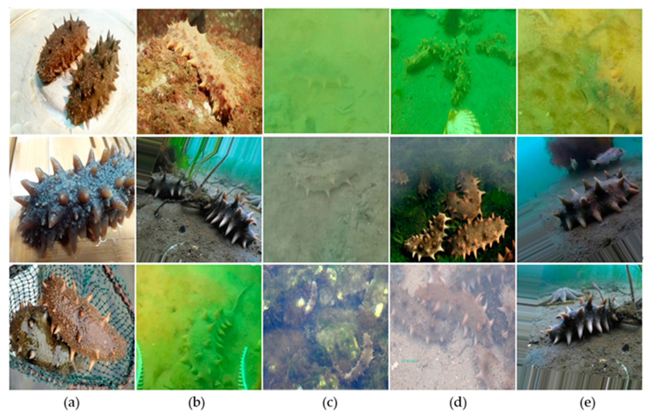
Figure 2.
The main network structure of YOLOv5, including the backbone network, the neck network, and the head network (the output module).
Figure 2.
The main network structure of YOLOv5, including the backbone network, the neck network, and the head network (the output module).
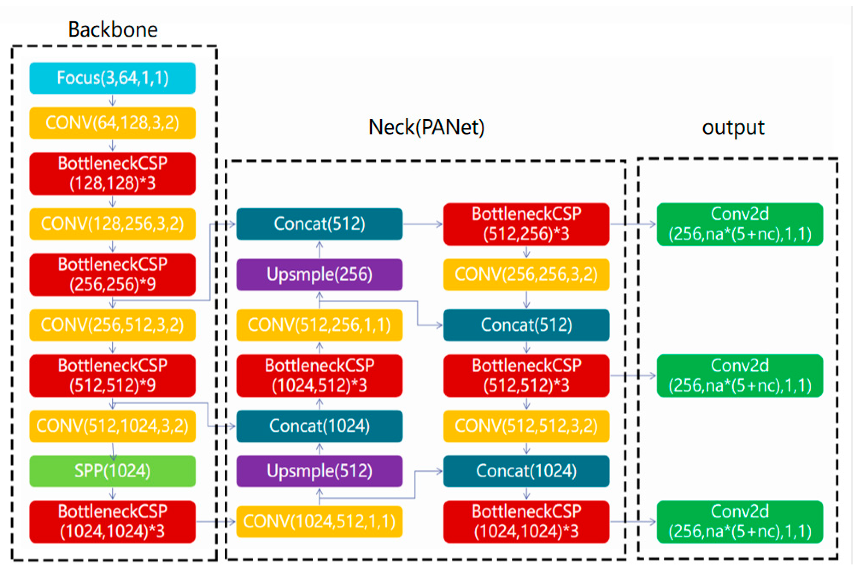
Figure 3.
The main structure of BottleneckCSP.
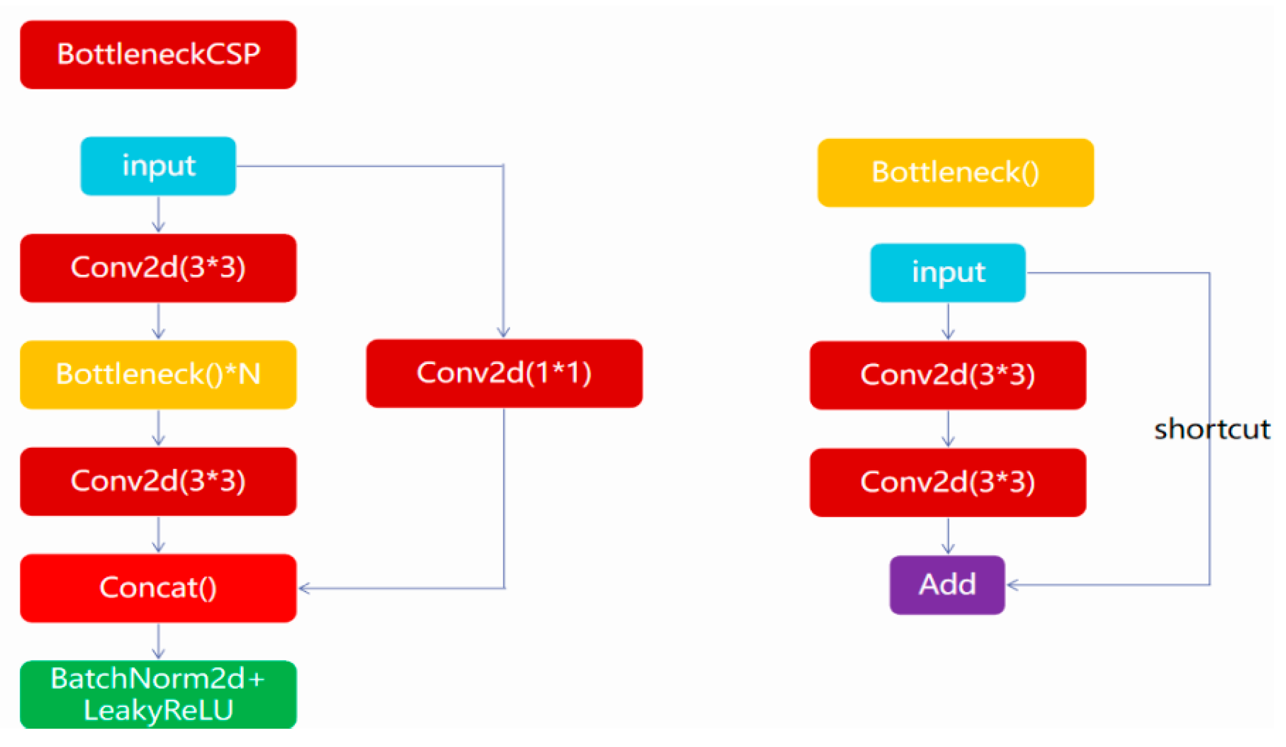
Figure 4.
The variation of the loss values, including: (a) the bounding box loss of the training set; (b) the object loss of the training set; (c) the classification loss of the training set; (d) the bounding box loss of the validation set; (e) the object loss of the validation set; (f) the classification loss of the validation set.
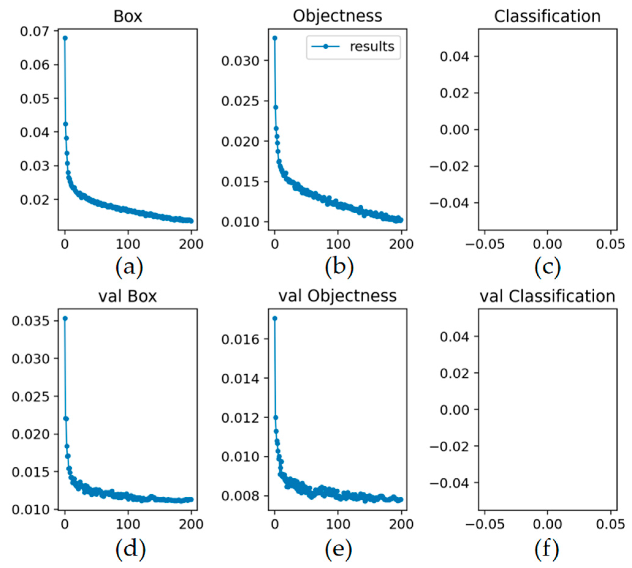
Figure 5.
The output of evaluation metrics: (a) Precision; (b) Recall; (c) MAP@0.5; (d) MAP@0.5:0.95; (e) Precision-recall curve; (f) F1 curve.
Figure 5.
The output of evaluation metrics: (a) Precision; (b) Recall; (c) MAP@0.5; (d) MAP@0.5:0.95; (e) Precision-recall curve; (f) F1 curve.
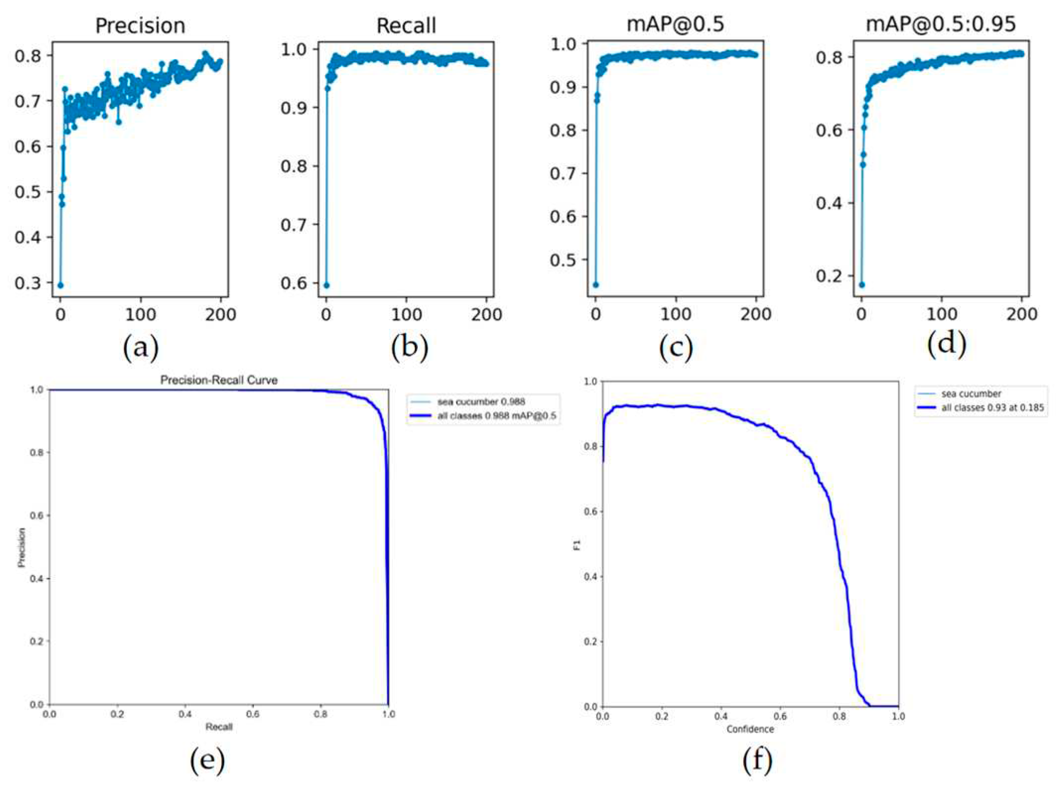
Figure 6.
Examples of the detection output.
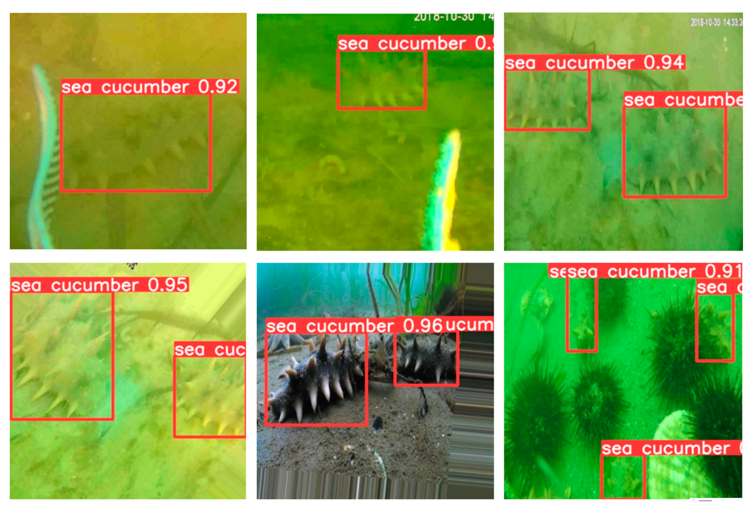
Figure 7.
The result of running the model on ROS of TX2.
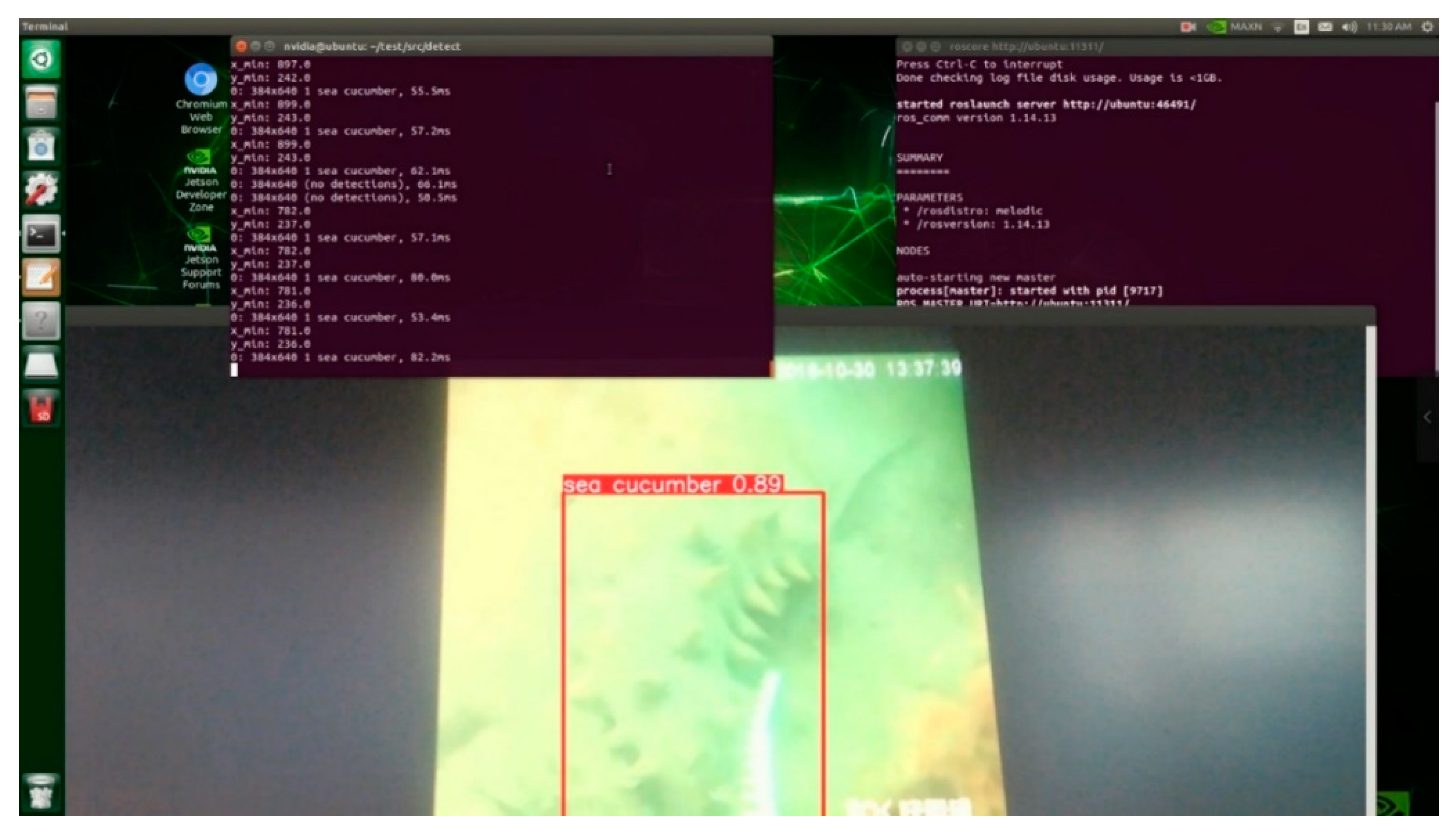
Figure 8.
Main flowchart of the DETR model.
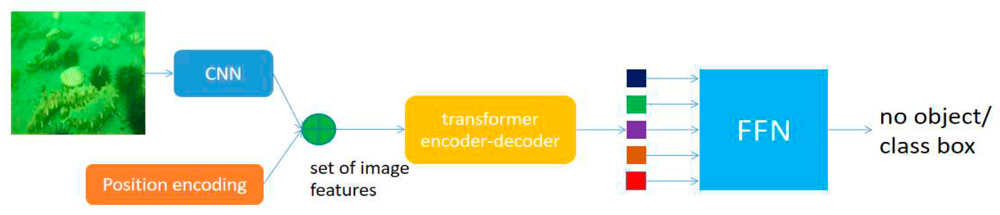
Figure 9.
Structure of the encoder-decoder model.
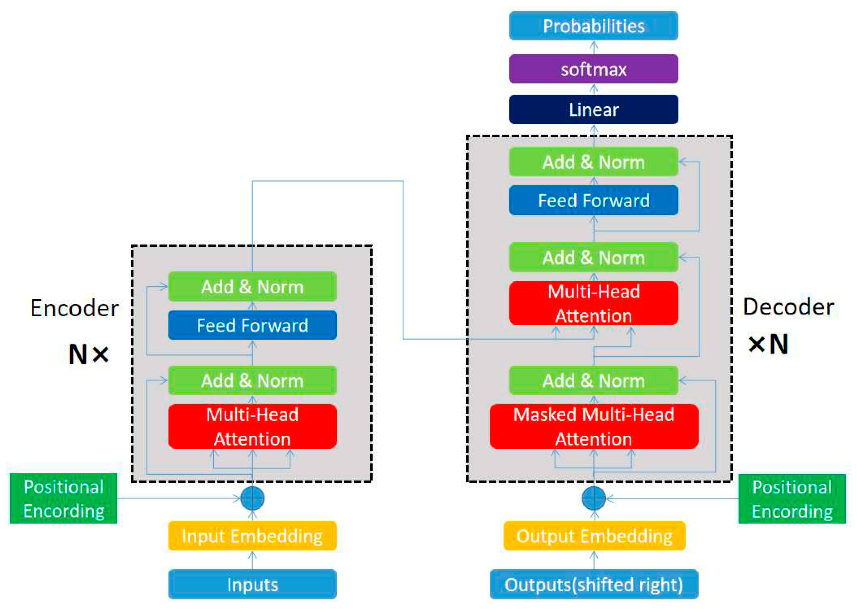
Figure 10.
The variation of the loss values. (a) The bounding box loss of the training set; (b) The total loss of the training set; (c) The bounding box loss of the validation set; (d) The total loss of the validation set; (e) The precision-recall curve.
Figure 10.
The variation of the loss values. (a) The bounding box loss of the training set; (b) The total loss of the training set; (c) The bounding box loss of the validation set; (d) The total loss of the validation set; (e) The precision-recall curve.
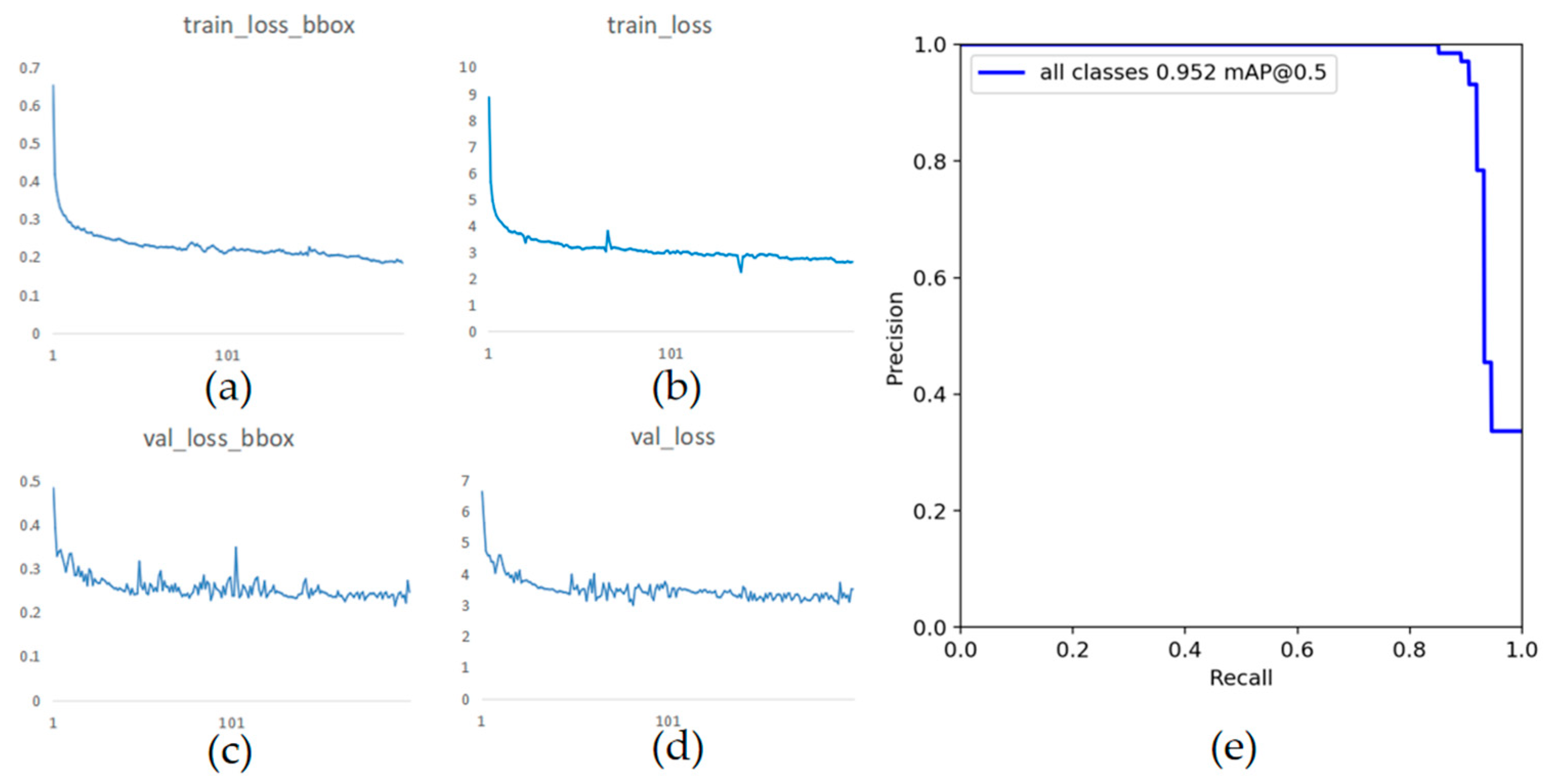
Figure 11.
Performance comparison on samples with different clarity. (a) Comparison under the value of mAP@0.5; (b) Comparison under the value of mAP@0.5:0.95.
Figure 11.
Performance comparison on samples with different clarity. (a) Comparison under the value of mAP@0.5; (b) Comparison under the value of mAP@0.5:0.95.
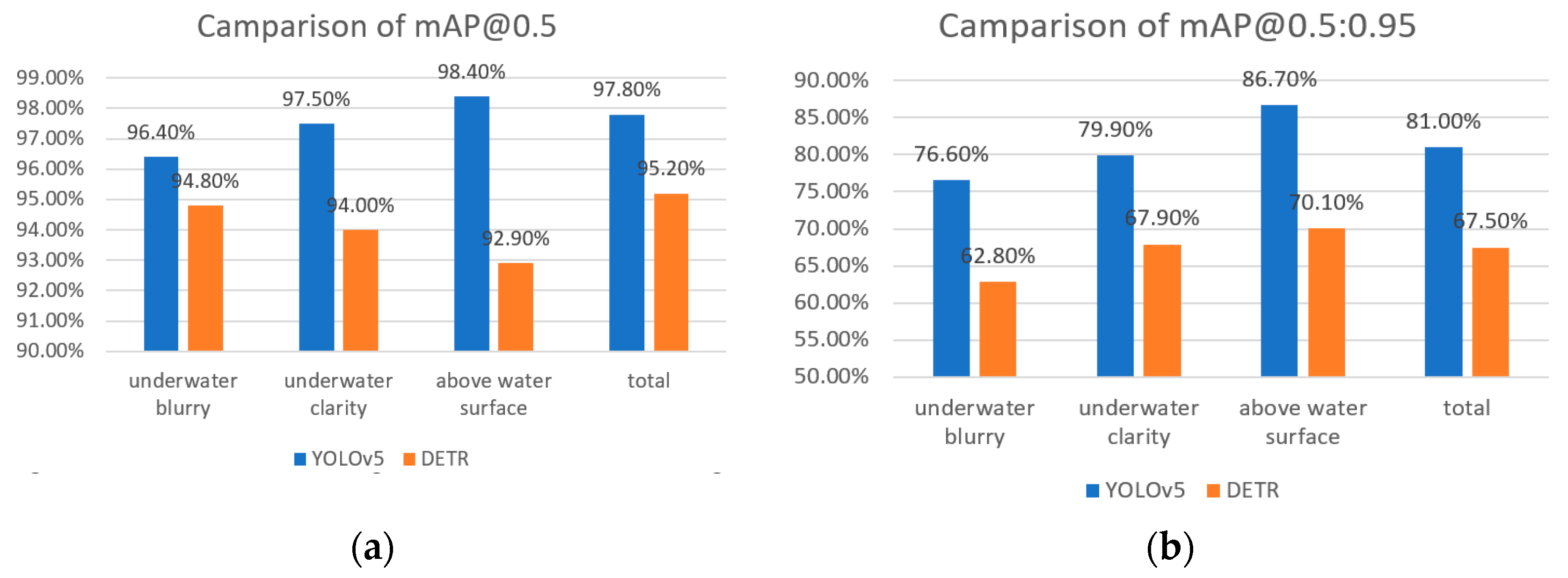
Figure 12.
Detection performances of the two algorithms. (a) Detection effect of samples above water surface; (b) Detection effect of samples in clear underwater area; (c) Detection effect of samples in turbid underwater zone.
Figure 12.
Detection performances of the two algorithms. (a) Detection effect of samples above water surface; (b) Detection effect of samples in clear underwater area; (c) Detection effect of samples in turbid underwater zone.
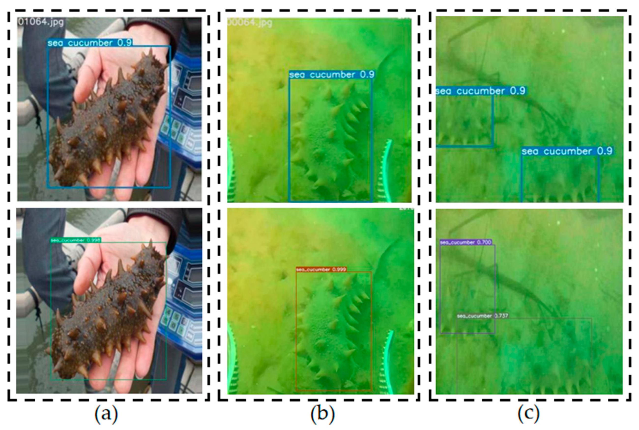
Figure 13.
Performance comparison on samples with different number of targets. (a) Comparison under the value of mAP@0.5; (b) Comparison under the value of mAP@0.5:0.95.
Figure 13.
Performance comparison on samples with different number of targets. (a) Comparison under the value of mAP@0.5; (b) Comparison under the value of mAP@0.5:0.95.
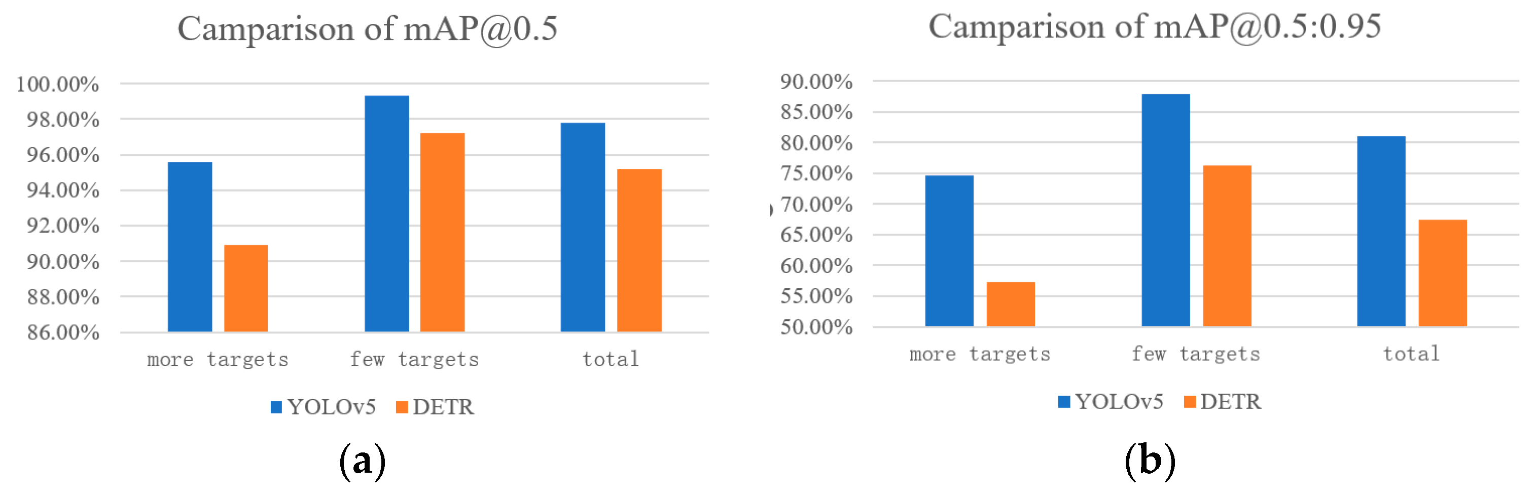
Figure 14.
Sample detection performance with multiple targets.
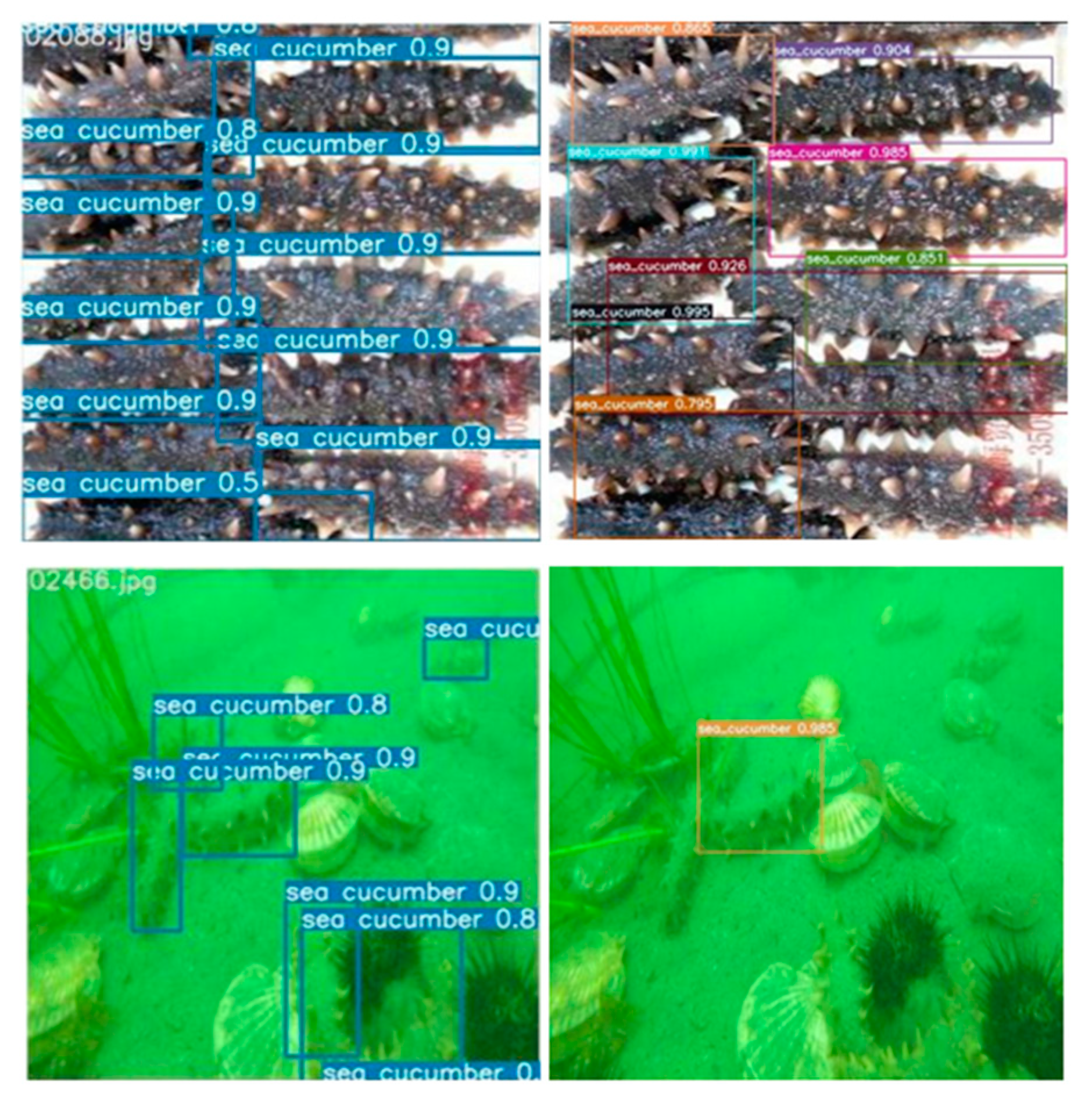

Table 1.
The computer configurations.
| Experimental Platform | Configuration |
|---|---|
| CPU | Intel(R) Core(TM) i7-9750H CPU @ 2.60GHz |
| GPU | NVIDIA GeForce RTX 2070 with Max-Q Design |
| RAM | DDR4 3000MHz 16G |
| Hard Drive | PCIE 3.0 NVME 512G |
| OS | Windows 10 |
| CUDA | 11.6 |
| Python | 3.9 |
Table 2.
Hyperparameter settings of network training.
| Training Epochs | Batch Size | Learning Rate (Initial) | Weight Decay |
|---|---|---|---|
| 98 | 32 | 0.01 | 0.0005 |
Table 3.
Test performance of YOLOv5 on various validation sets
| Precision | Recall | mAP@0.5 | mAP@0.5:0.95 | |
|---|---|---|---|---|
| above water surface | 88.9% | 97.3% | 98.4% | 86.7% |
| underwater clarity | 73.4% | 100% | 97.5% | 79.9% |
| underwater blurry | 76% | 96.1% | 96.4% | 76.6% |
| total | 78.1% | 97.5% | 97.8% | 81.0% |
Table 4.
Test performance of DETR on various validation sets
| Precision | Recall | mAP@0.5 | mAP@0.5:0.95 | |
|---|---|---|---|---|
| above water surface | 84.6% | 91.7% | 92.9% | 70.1% |
| underwater clarity | 74.1% | 95.4% | 94.0% | 67.9% |
| underwater blurry | 72.4% | 94.6% | 94.8% | 62.8% |
| total | 76.5% | 95.4% | 95.2% | 67.5% |
Table 5.
Test performance of YOLOv5 on various validation sets
| Precision | Recall | mAP@0.5 | mAP@0.5:0.95 | |
|---|---|---|---|---|
| More targets | 69.6% | 97.5% | 95.6% | 74.7% |
| Few targets | 93.2% | 98.3% | 99.3% | 87.9% |
| total | 78.1% | 97.5% | 97.8% | 81.0% |
Table 6.
Test performance of DETR on various validation sets
| Precision | Recall | mAP@0.5 | mAP@0.5:0.95 | |
|---|---|---|---|---|
| More targets | 60.1% | 91.2% | 90.9% | 57.3% |
| Few targets | 87.2% | 96.8% | 97.2% | 76.3% |
| total | 76.5% | 95.4% | 95.2% | 67.5% |
Disclaimer/Publisher’s Note: The statements, opinions and data contained in all publications are solely those of the individual author(s) and contributor(s) and not of MDPI and/or the editor(s). MDPI and/or the editor(s) disclaim responsibility for any injury to people or property resulting from any ideas, methods, instructions or products referred to in the content. |
© 2023 by the authors. Licensee MDPI, Basel, Switzerland. This article is an open access article distributed under the terms and conditions of the Creative Commons Attribution (CC BY) license (http://creativecommons.org/licenses/by/4.0/).
Copyright: This open access article is published under a Creative Commons CC BY 4.0 license, which permit the free download, distribution, and reuse, provided that the author and preprint are cited in any reuse.


