Submitted:
13 September 2023
Posted:
14 September 2023
You are already at the latest version
Abstract
A quantum particle constrained between two high potential barriers provides a paradigmatic example of a system sustaining quasi bound (or resonance) states. When the system is prepared in one of such quasi bound states, the wave function approximately maintains its shape but decays in time in a nearly exponential manner radiating into the surrounding space, the lifetime being of the order of the reciprocal of the width of the resonance peak in the transmission spectrum. Naively, one could think that adding more lateral barriers would preferentially slow down or prevent the quantum decay since tunneling is expected to become less probable and because of quantum backflow induced by multiple scattering processes. However, this is not always the case and in the early stage of the dynamics quantum decay can be accelerated (rather than decelerated) by additional lateral barriers, even when the barrier heights are arbitrarily large. The decay acceleration originates from resonant tunneling effects and is associated to large deviations from an exponential decay law. We discuss such a counterintuitive phenomenon by considering the hopping dynamics of a quantum particle on a tight-binding lattice with on-site potential barriers.
Keywords:
quantum tunneling
; quasi bound states
; tight binding lattices
1. Introduction
Quantum tunneling is ubiquitous in quantum mechanics where a particle has a non-zero probability of passing through a classically forbidden energy barrier, even though it doesn’t have enough energy to overcome that barrier according to classical physics [1,2]. This behavior arises from the wave-like nature of particles at the quantum level, and can be thus observed also for classical waves such as light and sound waves (see e.g. [3,4,5,6]). One of the main predictions of quantum tunneling is the instability and decay of a quantum particle trapped by potential barriers of finite heights, a prototypal example being -decay in nuclear physics [7,8]. Perhaps the simplest one-dimensional quantum mechanical model possessing quasi-stationary (resonance) states, decaying via tunneling leakage, is the double rectangular potential barrier model [Figure 1(a)], which was introduced in a famous paper by Gamov to model decay [7]. When the barrier height is infinite, the system sustains a set of stationary (non-decaying) bound states at some quantized energies, however when the barrier height is not infinite some of these states, those with energies close to the bottom of the barriers, become metastable, i.e. they become resonance states (also known as Gamow or Siegert states, or quasi-bound states; see e.g. [9,10,11,12,13,14] and references therein). This means that an initial wave function prepared in a bound state of the infinite barrier approximately maintains its shape but decays in time in a nearly exponential manner through tunneling leakage across the barriers, generating small-amplitude outgoing waves that spread outward the barrier region [9,10,11]. The signature of resonance states are the characteristic Breit-Wigner resonance peaks in the transmission spectrum of the double potential barrier, and the lifetimes of the resonance states are of the order of the reciprocal of the widths of the Breit-Wigner resonances [11] [see Figure 1(b)].
The quantum decay does not strictly follow a simple exponential decay law, and deviations from an exponential decay universally arise in the short and long time scales [15,16,17,18,19,20], leading to Zeno-like dynamics, i.e. the deceleration (Zeno effect) or the acceleration (anti-Zeno effect) of the decay by frequent observations of the system (see, e.g., [21,22,23,24,25] and references therein). Strong deviations from an exponential decay law are generally observed because of interference between different decay pathways, strong coupling with a featureless bath or with an engineered bath, which introduce memory effects and non-markovian behavior, or in the presence of edge effects or localized states, such as in disordered systems, leading to revivals and limited quantum decay [26,27,28].
Quantum leakage dynamics in the double-barrier potential is clearly modified when lateral barriers are added. Such additional barriers introduce interference effects and make the quantum decay greatly non-exponential rather generally. Naively, one could think that additional barriers would preferentially slow down the decay, since the tunneling is expected to become less probable and because of the back flow into the original excitation region. For example, for stochastic barriers one expects Anderson localization [29,30], leading to a highly non-markovian dynamics, Rabi-like oscillations and limited quantum decay [27,28,31]. However, this picture may fail in other cases as multiple interference effects could play in a reversed way.
In this work we unveil the rather counterintuitive effect of quantum decay acceleration of a resonance state in the double barrier model induced by additional later barriers: rather than slowing down the decay, they can greatly accelerate the quantum decay, even when the height of barriers are unbounded. This unusual phenomenon is explained in terms of resonant tunneling (hopping) and studied by considering in details the decay of resonance states in potential barriers on a tight-binding lattice, which can be emulated in photonic settings using evanescently-coupled optical waveguide lattices [32,33,34] or grating structures [35,36,37].
2. Acceleration and deceleration of quantum decay in the double barrier model: some preliminary considerations
Before considering quantum decay in tight-binding models with on-site potential barriers, it is worth presenting some preliminary results and discussion on the decay dynamics of resonance states in the Gamov’s model for the continuous Schrödinger equation in one spatial dimension, which is written in dimensionless units as
where is the wave function and is the potential. Let us first assume that describes a double rectangular barrier, with barrier height , barrier width b and barrier distance [Figure 1(a)]. Figure 1(b) shows a typical behavior of spectral transmittance versus energy E of the incidence plane wave. The transmission amplitude can be calculated by standard textbook methods and reads
where and are the reflection and transmission amplitudes of the single barrier, given by
and
The spectral transmittance clearly shows resonance peaks at some energies [two peaks at energies in the plot of Figure 1(b)], which correspond to quasi bound states. In the high-barrier limit, i.e. very narrow resonances [such as the first resonance at shown in the inset of Figure 1(b)], the resonance curve is Lorentzian-shaped to a high degree of approximation (Breit-Wigner resonance) and the corresponding quasi bound state can be roughly speaking written as
where , E are close to the bound state wave function and corresponding (possibly shifted) eigenenergy in the infinite limit, is the lifetime of the quasi bound state, is the full-width at half-maximum of the Breit-Wigner resonance, and describes the small-amplitude outgoing waves in the outer regions of the barriers [see Figure 1(a)]. An example of a nearly-exponential decay of the lowest resonance state is shown in Figure 2(b), which depicts the decay behavior of the survival probability to find the particle between the two barriers,
normalized to its initial value . Here, is assumed to be close to the lowest-energy bound state of the same barrier model but with , i.e. for and otherwise, propagated for a short time interval () to remove fast transient oscillations in the behavior of . The results are obtained by numerical integration of the time-dependent Schrödinger Equation (1) using an accurate pseudospectral split-step method. The decay dynamics [solid curve 1 in Figure 2(b)] is quite well fitted by an exponential curve [dashed curve 1 in Figure 2(b)] with a lifetime close to the theoretical value predicted from the spectral width of the lowest Breit-Wigner resonance peak. A similar behavior is found when the system is initially prepared in the second resonance state, i.e. for and otherwise, the exponential decay displaying a much shorter lifetime (), according to the larger width of the second resonance peak in Figure 1(b).
Clearly, the decay dynamics is greatly modified and can largely deviate from an exponential law when we consider additional lateral barriers, because the outgoing waves that escape via tunneling from the two barriers can be back reflected and re-injected into the original spatial region . The final decay law is the result of a complex multiple interference process which, depending on the choice of the additional barriers, can either decelerate or accelerate the decay. The fact that additional barriers can slow down the decay of the survival probability is not surprising, however it is more elusive how and why the decay can be accelerated in some cases. One of the main mechanism that explains decay acceleration is resonant tunneling (see e.g. [38]). This point can be illustrated by considering, as an example, the case of an array of equally-spaced barriers; see Figure 2(a). Besides the two barriers as in Figure 1(a), we now add a sequence of equally-spaced barriers of height , same space separation , and barrier width w. Barrier height and width w can be rather generally different than and a. Curves 2 and 3 in Figure 2(b) show the decay dynamics of the survival probability when either or both w and differ than b and , clearly indicating that the additional barriers decelerate the decay. However, a striking effect is observed when and : the decay of survival probability is much faster and the decay dynamics greatly deviates from an exponential law [curve 4 in Figure 2(b)]. The decay acceleration can be explained on the basis of resonant tunneling (hopping) between resonant quasi bound states that are sustained by adjacent double-potential barriers, as schematically shown in Figure 2(c). In fact, for and the potential is strictly periodic with period , and such a periodic potential corresponds to the well-known Kronig-Penney model in solid-state physics [39,40]. Basically, the various resonant quasi-bound states sustained in adjacent double-barriers hybridize and give rise to a set of bands. The dispersion curves of the various bands are defined implicitly by the relation (see e.g. [40])
where we have set
In the above equation, k is the Bloch wave number, which varies in the first Brillouin zone . The band dispersion curves, defined by the relation , can be solved graphically, as shown in Figure 2(d). The low-energy narrow-band in Figure 2(d), indicated as band 1 and centered at around , arises from the weak overlapping (hybridization) of resonant quasi-bound states with energies in adjacent unit cells of the crystal, and its bandwidth defines the hopping amplitude between adjacent sites within a tight-binding description. In the nearest-neighbor approximation, an initial excitation of one of such quasi-bound mode can jump from one unit cell to its neighbor in either direction with a rate , and the spreading dynamics is ballistic and governed by the set of coupled equations (see e.g. [40,41,42] )
where is the amplitude of the quasi bound state at the n-th unit cell. The decay behavior of the survival probability is then given analytically in terms of Bessel function, namely [41]
The solid curve 4 in Figure 2(b) shows the numerically-computed behavior of for and , which is very well fitted by the theoretical prediction given by Eq.(10) (dashed curve 4), in which the hopping rate is estimated from the width of the narrow band of Figure 2(d). Clearly, the decay of survival probability greatly deviates from an exponential curve and in the early stage it is much faster than other cases [curves 1-3 in Figure 2(b)], where resonant tunneling is prevented: the hopping dynamics enabled by resonant tunneling makes the decay faster.
3. Decay acceleration by resonant tunneling in tight-binding lattices
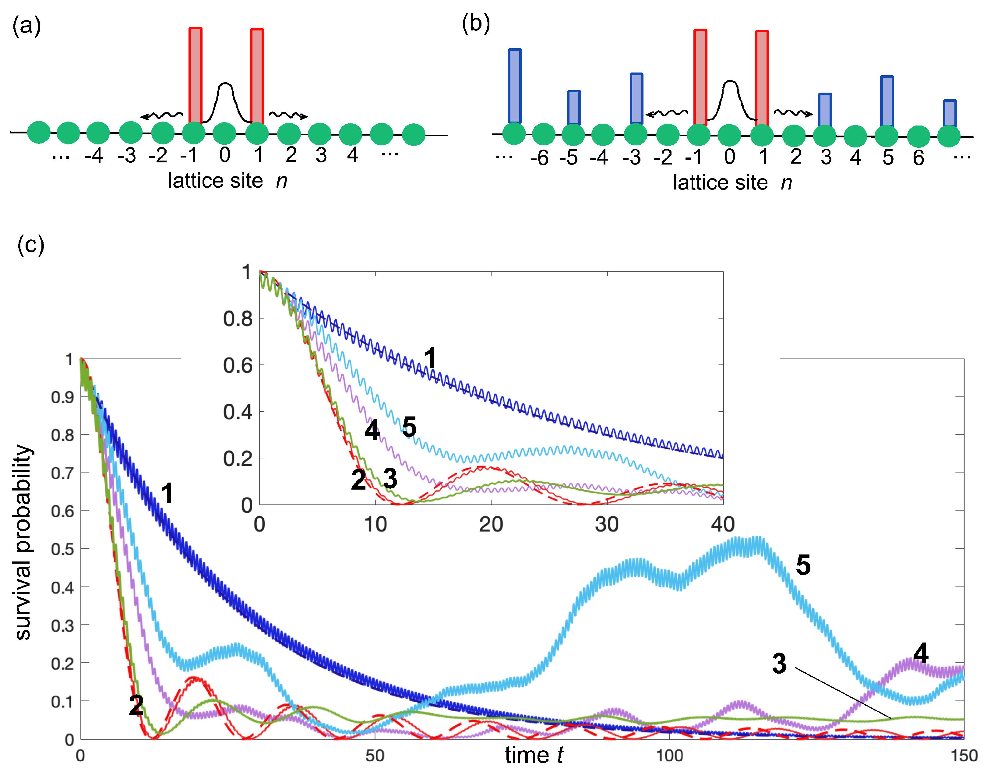
The phenomenon of decay acceleration in the early stage of the dynamics mediated by hopping between adjacent resonant quasi bound states, discussed in the previous section, suggests to re-examine quantum decay and tunneling effects in the framework of simple tight-binding models [32,43,44]. Such models, besides to be simpler to study and simulate, can be readily implemented in photonic settings using engineered arrays of evanescently-coupled optical waveguides. In fact, they have served over the past two decades as feasible laboratory tools for the observation of non-exponential decay features and Zeno dynamics with photons [5,33,34,45,46,47]. The simplest two-barrier system sustaining one resonance state on a tight-binding lattice is described by the Hamiltonian [Figure 3(a)]
where is the hopping rate between adjacent sites of the lattice and is the on-site potential barrier at the two sites . For the sake of definiteness we assume , however on a lattice a quasi bound state is also sustained for . Indicating by the wave amplitude at the n-th lattice site, i.e. after letting , the Schrödinger equation yields the set of coupled equations
In the high-barrier limit , an initial excitation at time of site , trapped between the two high potential barriers, is metastable and the survival probability, , decays in time nearly exponentially, as observed in numerical simulations of Eqs.(12) assuming the initial conditions ; see curve 1 in Figure 3(c). Note that a small-amplitude and fast oscillation is superimposed to the exponential decay, the amplitude of the oscillations vanishing in the limit. The lifetime of the quasi-bound state at site can be readily estimated by adiabatic elimination from the dynamics of the small amplitudes at the sites . In fact, in the high barrier limit one can assume in Eqs.(12) ,and thus
Taking into account for symmetry reasons that , after letting and for , from Eqs.(12) and (13) one obtains
where we have set
The reduced model (14) can be cast in the standard Friedrichs-Lee (or Fano-Anderson) model, describing the decay of a single bound state weakly coupled to a featureless tight-binding continuum (see e.g. [34,48,49]), and in the markovian approximation the survival probability can be calculated as
where the lifetime is given by (see Appendix A for details)
The exponential decay predicted by Eqs.(16) and (17) turns out to be in good agreement with the exact decay behavior found by numerical simulations [compare solid and dashed curves 1 in the inset of Figure 3(c)].
When lateral barriers are introduced, the decay dynamics is rather generally modified and does not follow anymore the exponential law Eq.(16). In order to observe decay acceleration by resonant tunneling as suggested in Sec.2 above, the potential barriers are added at odd potential sites solely; see Figure 3(b). The Hamiltonian of the system reads
where is the strength of the potential barrier at odd lattice sites, with and for n even. We mention that in photonics the tight-binding model (18) can be implemented using arrays of evanescently coupled optical waveguides, in which a uniform coupling constant and engineered propagation constant shifts are realized by judicious design of waveguide widths and spacing. For example, a linear gradient potential was realized in semiconductor waveguide arrays to demonstrate optical Bloch oscillations in Ref. [50].
After adiabatic elimination of the small amplitudes as discussed above [Eq.(13)], the decay dynamics of could be framed in the form of a single-level Fano-Anderson model, where the additional barriers clearly structure the continuum of states into which the state is coupled, and could induce localization phenomena responsible for strong backflow and revivals in the dynamics [26,27,28]. It is precisely these effects that make it possible decay acceleration in the early stage of the dynamics. The canonical Fano-Anderson form describing the decay process for the Hamiltonian (18) is detailed in the Appendix A, which derives the general form of the memory function entering in the integro-differential equation describing the decay dynamics of the amplitude . The memory function basically includes all the multiple reflection phenomena and delay effects arising from wave scattering of additional lateral barriers, which make the decay strongly non-markovian. The form of the memory function depends in a complex way on the eigenstates of the bath Hamiltonian, and even if its form might be calculated analytically in very special cases [51], it is hard to provide general insights into the decay dynamics as governed by the integro differential equation. However, for our purposes we do not need to resort to the canonical Fano-Anderson model and in the following analysis we will provide some direct examples of quantum decay acceleration adopting the full Hamiltonian (18). To this aim, it is worth noting that the system described by Eq.(18) is bipartite, and thus one can write the wave function as . The evolution equations for the wave amplitudes and at even and odd lattice sites read
which should be solved with the initial condition and .
Let us now discuss a few prototypal examples of decay acceleration, observed in the early stage of the dynamics, induced by the additional lateral barriers.
(i) The first example of decay acceleration is obtained by assuming for n odd, which is the discrete analogue of the Kronig-Penney model considered in the previous section [Figure 2(c)]. In this case the Hamiltonian (18) describes a bipartite lattice sustaining two bands. In the high barrier limit , to calculate the decay of the survival probability we can adiabatically eliminate the small amplitudes from the dynamics by letting
so that from Eq.(19) one obtains
where we have set
The solution to Eq.(22) with the initial condition is given in terms of Bessel function [41,42] and the corresponding decay behavior of the survival probability reads
Curve 2 in Figure 3(c) shows the numerically-computed decay behavior of for , which turns out to be quite well fitted by the theoretical prediction given by Eq.(24). Clearly, the decay largely deviates from an exponential law and, most importantly, it is accelerated as compared to curve 1, at least in the early-to-intermediate time scale of the decay.
(ii) As a second example of decay acceleration, let us assume that at odd sites n, with , the potential can take two possible values, either or , with probabilities p and , respectively (Bernoulli model [52]). Curve 3 in Figure 3(c) shows the numerically-computed decay behavior of the survival probability for , , and , averaged over 200 realizations. Also in this case one can clearly observe an acceleration of the decay in the early stage of the dynamics, in spite of Anderson localization can take place in this model (see Appendix B). This means that, unlike the previous example (i), at long times the decay is not complete.
(iii) The third example of decay acceleration concerns with deterministic potential barriers with continuously-increasing and unbounded heights, namely we assume symmetric Stark potential barriers with and
Curve 4 in Figure 3(c) shows the numerically-computed behavior of the survival probability for and , clearly showing the acceleration of the decay in early stage of the decay. This is a rather striking and unexpected result, given that the added barriers have a monotonously increasing and unbounded height and the corresponding Hamiltonian (18) has an almost pure point spectrum with localized eigenstates (see Appendix B and [53]).
(iv) The fourth example of decay acceleration is analogous to the previous case, but with a quadratic (rather than linear) increase of barrier heights, i.e. we assume and
Curve 5 in Figure 3(c) shows the numerically-computed behavior of the survival probability for and , clearly showing the acceleration of the decay in early stage, with strong revival at longer times.
It should be remarked that decay acceleration mediated by the resonant tunneling effect, observed in all above models, occurs only in the early stage of the dynamics, as shown in Figure 3(c). In fact, at long times the the survival probability can become smaller when there are no additional lateral barriers, because the backflow arising from multiple scattering processes and localization effects, responsible for strong non-markovianity and deviation of the decay from an exponential curve, induce revival effects in the survival probability, which are prevented in the simple two-barrier case.
4. Conclusion
The decay of a resonance state trapped in a double potential barrier provides one of the simplest models of unstable quantum systems, which was introduced in a landmark paper by Gamov to explain decay in nuclear physics. A main question, which has been so far largely overlooked, is whether quantum decay of a metastable state in the double-barrier model can be accelerated by additional lateral barriers. Such additional barriers clearly induce multiple scattering and interference effects, that greatly modify the decay dynamics: the outgoing waves that escape via tunneling from the two barriers can be back reflected and re-injected into the original spatial region by the later barriers. The resulting decay behavior can strongly deviate from an exponential law and is the result of a complex multiple interference process which, depending on the choice of the additional barriers, can either decelerate or accelerate the decay. The fact that additional barriers can slow down the decay of the survival probability is not surprising, however it is more elusive how and why the decay can be accelerated in some cases. In this work we have shown that a main mechanism that can induce decay acceleration, at least in the early stage of the decay, is resonant tunneling. We have illustrated such a phenomenon by considering in details the decay dynamics of resonant states in tight binding models, showing that decay acceleration can be observed even when the later barriers are increasingly higher and higher or have some stochastic distribution. The predicted effects could be observable in photonic tunneling experiments using engineered integrated waveguide array circuits.
Funding
This research was funded by Agencia Estatal de Investigacion (MDM-2017-0711).
Data Availability Statement
No data were generated or analyzed in the presented research.
Conflicts of Interest
The authors declare no conflict of interest.
Appendix A. Fano-Anderson form of the quantum decay on the lattice
In this Appendix we derive the canonical Fano-Anderson (or Friedrichs-Lee) form of the quantum decay on the lattice described by the Hamiltonian (18). After letting , the evolution equations for the amplitudes read
For the sake of simplicity, we assume that the potential is symmetric around , i.e. . In this case, for the initial condition , the solution to Eq.(A1) satisfies the constraint , so that we can limit to consider the evolution equations for the amplitudes , , , ... which read explicity
In the large limit, we can adiabatically eliminate from the dynamics the amplitude by assuming in Eq.(A3). This yields
After letting
from Eqs.(A1-A7) one obtains
where we have set
To obtain the canonical form of Fano-Anderson model, let us indicate by
and the eigenvectors and corresponding eigenvalues (energies) of the semi-infinite matrix Hamiltonian , defined by
where is a discrete index (for localized states) or a continuous variable (for extended states). The eigenstates are assumed to satisfy the orthonormal condition for discrete indices (point spectrum), or for continuous indices (continuous spectrum). After expanding the amplitudes as a series (or integral) of the eigenstates of , i.e. after letting
from Eqs.(A8-A10) and (A13) one readily obtains the following set of evolution equations
where we have set
In Eqs.(A13) and (A14), it is understood that the sum over should be replaced by an integral over for the continuous part of the spectrum of . In their present form, Eqs.(A14) and (A15) can be derived from the single-level Fano-Anderson (or Friedrichs-Lee) Hamiltonian [24,48,49]
which describes the decay of a single level of frequency coupled to a discrete or continuous set of states (the bath), with frequencies , by a spectral coupling function . We mention that, in the most general case where the parity condition is not satisfied, one can still obtain a Fano-Anderson Hamiltonian as Eq.(A16), but the level turns out to be coupled to two baths with different spectral coupling functions.
After eliminating from the dynamics the variables by formally solving Eq.(A15) with the initial condition and after letting , from Eq.(14) one obtains the following integro-differential equation describing the decay dynamics of the amplitude
where is the memory function, defined by
Only when the single level is weakly coupled to a featureless continuum of states with a short memory time – the memory time is the characteristic decay time of the memory function – one can use the markovian (or Weisskopf-Wigner) approximation [22], and the decay dynamics is well described by an exponential law. In this case Eq.(A18) reduces to a simple differential equation, i.e.
where we have set defining the Lamb shift () and decay rate (). After letting in Eq.(A18) and following a standard procedure, the explicit form of the decay rate and Lamb shift can be calculated as
where is the spectral coupling function and is the density of states.
As an example of a nearly-exponential decay, let us consider the quantum decay in the absence of lateral barriers, i.e. with , corresponding to in Eq.(A12). In this case the spectrum of the matrix Hamiltonian [Eq.(A12)] is absolutely continuous, and neglecting the small defect (impurity potential) at the edge, its energy spectrum and corresponding eigenfunctions read (see e.g. [49])
where is a continuous parameter. In this case, the spectral coupling function and density of states are readily calculated as
Taking into account that , from Eqs.(A20) and (A22) one obtains
and thus the lifetime reads
which is Eq.(17) given in the main text.
Appendix B. Some qualitative properties of the energy spectrum and weak localization
In this Appendix we present some discussion about the energy spectrum of the tight-binding bipartite Hamiltonian H defined by Eq.(18) in the main text. After letting , from Eqs.(19) and (20) one obtains the spectral problem
It can be readily shown that the energy belongs to the spectrum of H with wave function in one sublattice solely
corresponding to an extended (improper) eigenstate. For , from Eq.(A25) one can express the amplitudes in one sublattice in terms of the amplitudes in the other sublattice, i.e.
Substitution of Eq.(A28) into Eq.(A26), after letting one obtains
Equation (A29) can be regarded as the spectral problem on a tight-binding lattice in the potential with an energy-dependent amplitude, vanishing as .
Clearly, if is constant, like in the example (i) considered in Sec.3, or a periodic function of index n, the energy spectrum is absolutely continuous and H does not sustain any localized state. In this case we expect the decay of survival probability to be complete. Conversely, if describes some disordered potential, such as the Anderson-Bernoulli model [52] considered in the example (ii) of Sec.3, or a deterministic potential with monotonously increasing and unbounded as , such as the symmetric Stark potential or the parabolic potentials discussed in the examples (iii) and (iv) of Sec.3, all eigenstates with are strictly speaking localized. This is because any uncorrelated disordered potential of arbitrarily small amplitude in one dimension, or any unbounded potential of small amplitude which is monotonously increasing with , have all eigenstates localized. However, an infinitely countable set of eigenenergies, with weakly extended eigenstates, accumulate toward the zero energy point of the extended state, with a diverging localization length of corresponding eigenstates. Such a property can be proven rigorously in some special potential models, such as the Stark potential model [53] or other integrable models such as the Maryland model [54]. More generally, for small energies the potential entering in Eq.(A5) is almost vanishing and thus we expect that any eigenstate, if localized, should have a large localization length, diverging as . For random potentials, this result, i.e. the divergence of the localization length as , is rigorously proven in [55]. Interestingly, from Eq.(A28) it follows that the occupation of the eigenstates with energy close to zero is mostly restricted to one sublattice, namely . Such weakly-localized eigenstates are nearly resonant with the quasi-bound state localized at site , between the two high barriers. The quasi bound state can thus couple with such weakly localized states, while other strongly localized states with high energy do not play any main role in the decay dynamics. This means that the decaying quasi-bound state couples to a set of discrete and weakly-localized states of the bath, which is responsible rather generally for memory (non-markovian) effects and strong deviations from an exponential decay law. This explains why the long-time dynamics displays strong revival effects and also limited decay, such as those observed in models (iii), (iv) and (v) discussed in the main text [see Figure 3(c)]. References
References
- Merzbacher, E. The Early History of Quantum Tunneling. Phys. Today 2002, 55, 44. [Google Scholar] [CrossRef]
- M. Razavy, Quantum Theory of Tunneling, World Scientific, Singapore (2003).
- I. Vorobeichik, E. Narevicius, G. Rosenblum, M. Orenstein, and N. Moiseyev, Electromagnetic Realization of Orders-of-Magnitude Tunneling Enhancement in a Double Well System. Phys. Rev. Lett. 2003, 90, 176806. [CrossRef] [PubMed]
- G. Della Valle, M. Ornigotti, E. Cianci, V. Foglietti, P. Laporta, and S. Longhi, Visualization of Coherent Destruction of Tunneling in an Optical Double Well System. Phys. Rev. Lett. 2007, 98, 263601. [CrossRef] [PubMed]
- Longhi, S. Quantum-optical analogies using photonic structures. Laser & Photon. Rev. 2009, 3, 243. [Google Scholar]
- Geng, Z.; Maasilta, I.J. Complete tunneling of acoustic waves between piezoelectric crystals. Commun. Phys. 2023, 6, 178. [Google Scholar] [CrossRef]
- Gamow, G. Zur Quantentheorie des Atomkernes. Zeit. Phys. 1928, 51, 204. [Google Scholar] [CrossRef]
- Gurney, R.W.; Condon, E.U. Quantum Mechanics and Radioactive Disintegration. Nature 1928, 122, 439. [Google Scholar] [CrossRef]
- Klaiman, S.; Gilary, I. On Resonance: A First Glance into the Behavior of Unstable States. Adv. Quantum Chem. 2012, 63, 1. [Google Scholar]
- García-Calderón, G. Theory of resonant states: and exact analytical approach for open quantum systems. Adv. Quantum Chem. 2010, 60, 407. [Google Scholar]
- Jakobovits, H.; Rothschild, Y.; Levitan, J. The approximation to the exponential decay law. Am. J. Phys. 1995, 63, 439. [Google Scholar] [CrossRef]
- Moiseyev, N. Quantum theory of resonances: calculating energies, widths and cross-sections by complex scaling. Phys. Rep. 1998, 302, 211. [Google Scholar] [CrossRef]
- A. del Campo, G. García-Calderòn, and J.G. Muga, Phys. Rep. 2009, 476, 1.
- Gadella, M.; Fortin, S.; Jorge, J.P.; Losada, M. Mathematical Models for Unstable Quantum Systems and Gamow States. Entropy 2022, 24, 804. [Google Scholar] [CrossRef] [PubMed]
- Winter, R.G. Evolution of a Quasi-Stationary State. Phys. Rev. 1961, 123, 1503. [Google Scholar] [CrossRef]
- Fonda, L.; Ghirardi, G.C.; Rimini, A. Decay theory of unstable quantum systems. Rep. Prog. Phys. 1978, 41, 587. [Google Scholar] [CrossRef]
- Nakazato, H.; Namiki, M.; Pascazio, S. Temporal behavior of quantum mechanical systems. Int. J. Mod. Phys. B 1996, 10, 247. [Google Scholar] [CrossRef]
- S.R. Wilkinson, C.F. Bharucha, M.C. Fischer, K.W. Madison, P.R. Morrow, Q. Niu, B. Sundaram, and M.G. Raizen, Experimental evidence for non-exponential decay in quantum tunnelling. Nature 1997, 387, 575.
- E. Torrontegui, J.G. Muga, J. Martorell, and D.W.L. Sprung, Quantum Decay at Long Times. Adv. Quantum Chem. 2010, 60, 485.
- M. Peshkin, A. Volya, and V. Zelevinsky, Non-exponential and oscillatory decays in quantum mechanics. EPL 2014, 107, 40001. [CrossRef]
- Misra, B.; Sudarshan, E.C.G. Zeno paradox in quantum dynamics. J. Math. Phys. 1977, 18, 756. [Google Scholar] [CrossRef]
- Kofman, A.G.; Kurizki, G. Acceleration of quantum decay processes by frequent observations. Nature 2000, 405, 546. [Google Scholar] [CrossRef]
- M. C. Fischer, B. Gutiérrez-Medina, and M. G. Raizen, Observation of the Quantum Zeno and Anti-Zeno Effects in an Unstable System. Phys. Rev. Lett. 2001, 87, 040402. [CrossRef]
- P. Facchi, H. Nakazato, and S. Pascazio, From the Quantum Zeno to the Inverse Quantum Zeno Effect. Phys. Rev. Lett. 2001, 86, 2699. [CrossRef] [PubMed]
- Kofman, A.G.; Kurizki, G. Universal Dynamical Control of Quantum Mechanical Decay: Modulation of the Coupling to the Continuum. Phys. Rev. Lett. 2001, 87, 270405. [Google Scholar] [CrossRef] [PubMed]
- Gaveau, B.; Schulman, L. S. Limited quantum decay. J. Phys. A: Math. Gen. 1995, 28, 7359. [Google Scholar] [CrossRef]
- S. Lorenzo, F. Ciccarello, and G.M. Palma, Non-Markovian dynamics from band edge effects and static disorder. Int. J. Quantum Inform. 2017, 15, 1740026. [CrossRef]
- S. Lorenzo, F. Lombardo, F. Ciccarello, and G. M. Palma, Quantum non-Markovianity induced by Anderson localization. Sci. Rep. 2017, 7, 42729. [CrossRef] [PubMed]
- Rojas-Molina, C. Random Schrödinger operators and Anderson localization in aperiodic media. Rev. Math. Phys. 2020, 32, 2060010. [Google Scholar] [CrossRef]
- I. F. Herrera-González, F. M. Izrailev, and N. M. Makarov, Resonant enhancement of Anderson localization: Analytical approach. Phys. Rev. E 2013, 88, 052108. [CrossRef] [PubMed]
- G.L. Giorgi, S. Lorenzo, and S. Longhi, Topological Protection and Control of Quantum Markovianity. Photonics 2020, 7, 18. [CrossRef]
- Longhi, S. Nonexponential Decay Via Tunneling in Tight-Binding Lattices and the Optical Zeno Effect. Phys. Rev. Lett. 2006, 97, 110402. [Google Scholar] [CrossRef]
- F. Dreisow, A. Szameit, M. Heinrich, T. Pertsch, S. Nolte, A. Tünnermann, and S. Longhi, Decay Control via Discrete-to-Continuum Coupling Modulation in an Optical Waveguide System. Phys. Rev. Lett. 2008, 101, 143602. [CrossRef] [PubMed]
- P. Biagioni, G. Della Valle, M. Ornigotti, M. Finazzi, L. Duó, P. Laporta, and S. Longhi, Experimental demonstration of the optical Zeno effect by scanning tunneling optical microscopy. Opti. Express 2008, 16, 3762. [CrossRef]
- S. Longhi, P. Laporta, M. Belmonte, and E. Recami, Measurement of superluminal optical tunneling times in double-barrier photonic band gaps. Phys. Rev. E 2002, 65, 046610. [CrossRef]
- Longhi, S. Classical simulation of relativistic quantum mechanics in periodic optical structures. Appl. Phys. B 2011, 104, 453. [Google Scholar] [CrossRef]
- D Janner, G Galzerano, G Della Valle, P Laporta, S Longhi, M Belmonte, Slow light in periodic superstructure Bragg gratings. Phys. Rev. E 2005, 72, 056605. [CrossRef]
- J. Le Deunff, O. Brodier, and A. Mouchet, A primer for resonant tunnelling. Eur. J. Phys. 2012, 33, 1771. [CrossRef]
- R. de L. Kronig and W.G. Penney, Quantum Mechanics of Electrons in Crystal Lattices. Proc. Roy. Soc. A 1930, 130, 499.
- C. Kittel, Introduction to Solid State Physics, 8th ed. (Wiley, New York, 2005).
- D. H. Dunlap and V. M. Kenkre, Dynamic localization of a charged particle moving under the influence of an electric field. Phys. Rev. B 1986, 34, 3625. [CrossRef] [PubMed]
- F.A. Cuevas, S. Curilef, and A.R. Plastino, Spread of highly localized wave-packet in the tight-binding lattice: Entropic and information-theoretical characterization. Ann. Phys. 2011, 326, 2834. [CrossRef]
- Longhi, S. Tunneling escape in optical waveguide arrays with a boundary defect. Phys. Rev. E 2006, 74, 026602. [Google Scholar] [CrossRef] [PubMed]
- Longhi, S. Photonic simulation of giant atom decay. Opt. Lett. 2020, 45, 3017. [Google Scholar] [CrossRef] [PubMed]
- A. Crespi, F.V. Pepe, P. Facchi, F. Sciarrino, P. Mataloni, H. Nakazato, S. Pascazio, and R. Osellame, Experimental Investigation of Quantum Decay at Short, Intermediate, and Long Times via Integrated Photonics. Phys. Rev. Lett. 2019, 122, 130401. [CrossRef] [PubMed]
- Q. Liu, W. Liu, K. Ziegler, and F. Chen, Engineering of Zeno Dynamics in Integrated Photonics. Phys. Rev. Lett. 2023, 203, 103801.
- S.K. Ivanov, S.A. Zhuravitskii, N.N. Skryabin, I.V. Dyakonov, A.A. Kalinkin, S.P. Kulik, Y.V. Kartashov, V.V. Konotop, and V.N. Zadkov. Macroscopic Zeno effect in Su-Schrieffer-Heeger photonic topological insulator. arXiv 2023, arXiv:2308.00523.
- G. Sudarshan, in Field Theory, Quantization and Statistical Physics, edited by E. Tirapegui (Reidel, Dordrecht, 1988), pp. 237-245.
- Longhi, S. Bound states in the continuum in a single-level Fano-Anderson model. Eur. Phys. J. B 2007, 57, 45. [Google Scholar] [CrossRef]
- R. Morandotti, U. Peschel, J. S. Aitchison, H. S. Eisenberg, and Y. Silberberg, Experimental Observation of Linear and Nonlinear Optical Bloch Oscillations. Phys. Rev. Lett. 1999, 83, 4756. [CrossRef]
- Longhi, S. Optical analogue of coherent population trapping via a continuum in optical waveguide arrays. J. Mod. Opt. 2009, 56, 729. [Google Scholar] [CrossRef]
- R. Carmona, A. Klein, and F. Martinelli, Anderson Localization for Bernoulli and Other Singular Potentials. , 1987, 108, 41.
- Longhi, S. Absence of mobility edges in mosaic Wannier-Stark lattices. Phys. Rev. B 2023, 108, 064206. [Google Scholar] [CrossRef]
- J. He, X. Xia, Arithmetic phase transitions for mosaic Maryland model. J. Math. Phys. 2023, 64, 043504. [CrossRef]
- H. Matsuda and K. Ishii, Localization of Normal Modes and Energy Transport in the Disordered Harmonic Chain. Suppl. Prog. Theor. Phys. 1970, 45, 56. [CrossRef]
Figure 1.
(a) Schematic of a double rectangular potential barrier sustaining resonance (quasi-bound) states at energies . Barrier height is , barrier width is b and barrier distance is . (b) Spectral transmittance of the two-barrier potential versus energy of the incidence wave. Parameter values are , . The inset in (b) shows an enlargement of the first resonance at energy , which is well approximated by a Lorentzian curve (Breit-Wigner resonance). The two resonance peaks in (b) correspond to the quasi bound states depicted in (a) by the solid red curves. In the high potential barrier limit, the quasi bound state can be approximately written as in Eq.(6), where describes the small-amplitude outgoing waves escaping from the barrier region owing to evanescent tunneling (oscillating tails in the plots) and is the lifetime, which is the inverse of the width of the corresponding resonance peak in (b).
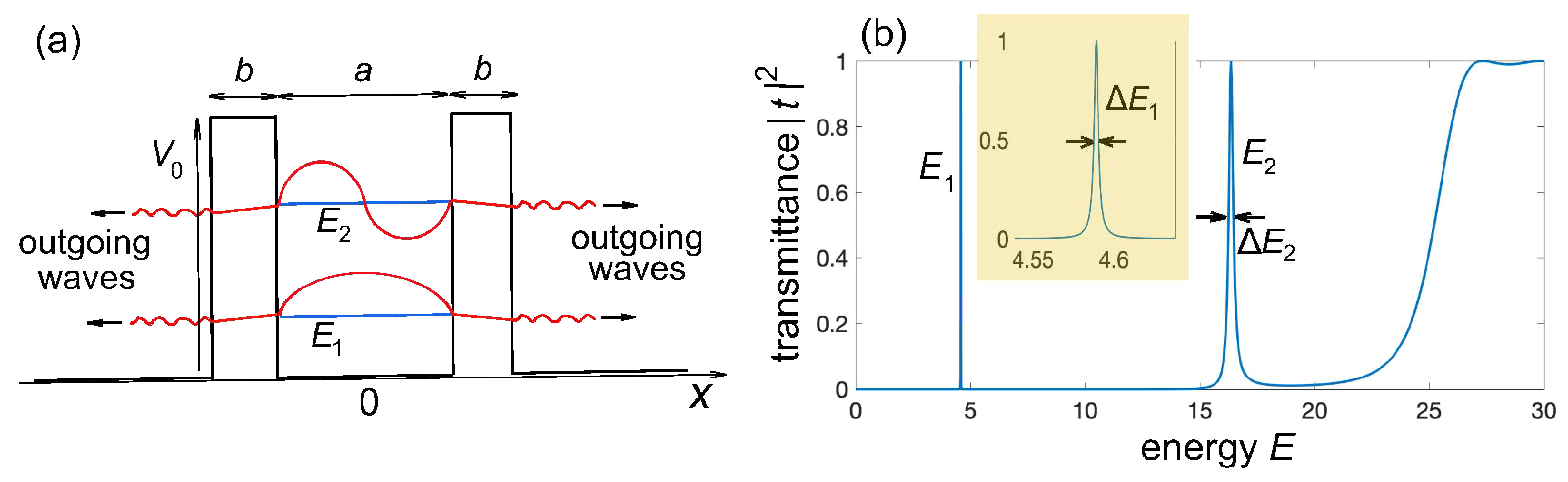
Figure 2.
(a) Schematic of a quasi bound state in the double barrier model (bold solid curve), that radiates in space with additional later barriers (thin solid curves). All barriers are equally spaced by a distance d. The size w and height of the lateral barriers can differ than those of the two central barriers. (b) Numerically-computed decay behavior of the survival probability , normalized to its initial value , for , , , and for a few different values of w and . Curve 1: quasi bound state radiating in free space (); the dashed curve is the exponential decay law with lifetime predicted by the width of the first resonance peak in the spectrum of Figure 1(b). Curve 2: , . Curve 3: , . Curve 4: , ; the dashed curve 4 is the decay behavior predicted by the tight-binding analysis of resonant tunneling [Eq.(10)]. (c) The Kronig-Penney model for and . The set of resonant quasi-bound states trapped in adjacent double-barrier potentials form an energy band, and excitation can hop between adjacent cells of the crystal with a hopping rate . (d) Geometrical construction of the energy bands for the Kronig-Penney model. The solid curve shows the behavior of the function versus energy E; the function is defined by Eq.(8) in the main text. The allowed energy bands are determined by the inequality and are indicated as band 1, band 2, band 3 in the figure. The narrow band 1 arises from the hybridization of the lowest-energy resonant quasi bound states sustained by each double potential barrier (unit cell) in the crystal.
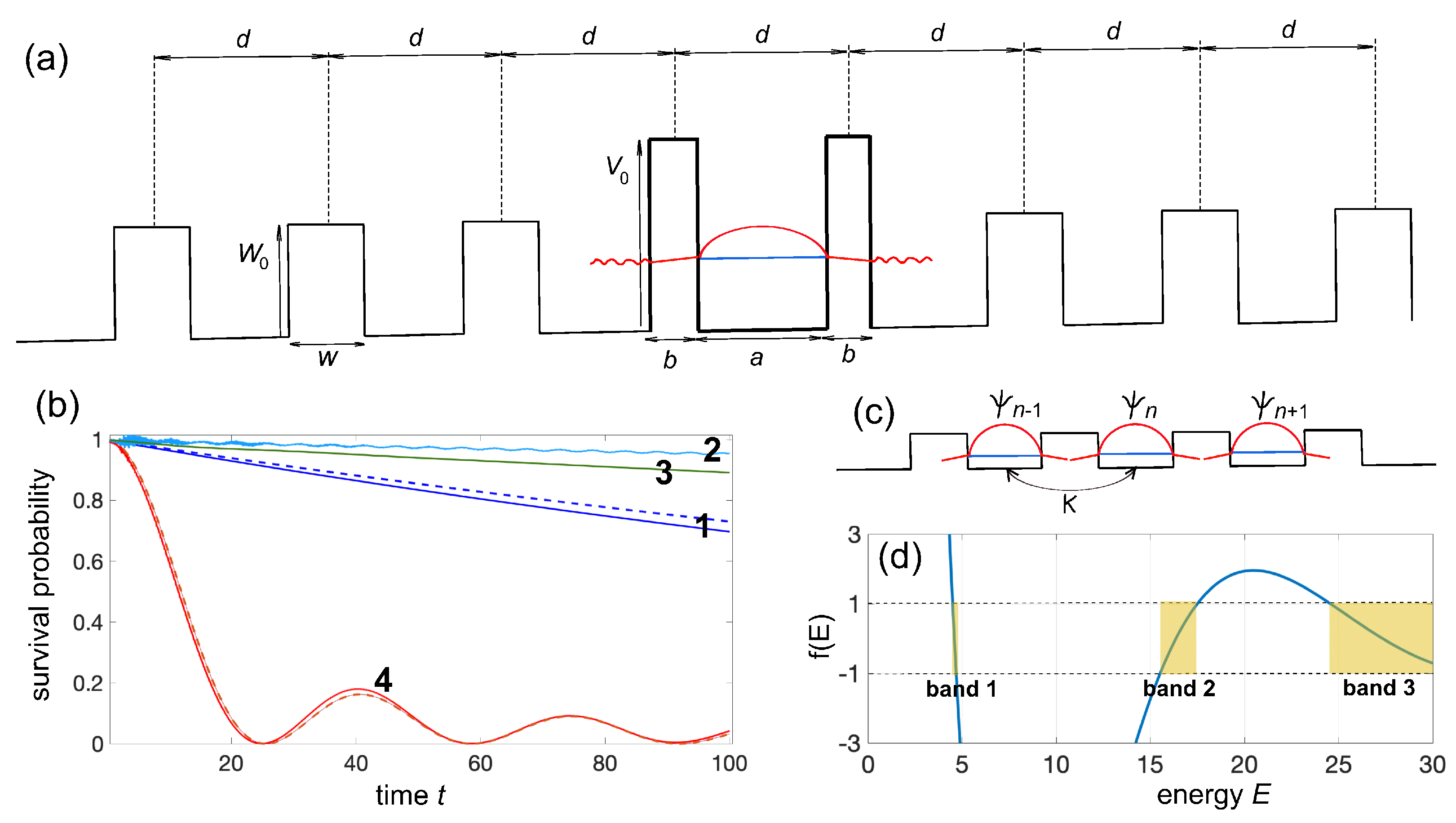
Figure 3.
(a) Schematic of a double barrier potential on a tight-binding lattice. A quasi-bound state trapped between the two high barriers radiates into the lattice. (b) The multi-barrier model. Additional potential barriers are introduced at odd lattice sites. (c) Decay of the survival probability for a few different settings of potential barriers and for , . Curve 1 is the nearly-exponential decay behavior of the double-barrier model of panel (a), i.e. in the absence of additional lateral barriers. The almost overlapped dashed curve is the exponential decay law predicted by Eq.(16). Curve 2 is the decay curve obtained for , and the almost overlapped dashed curve is the theoretical prediction given by Eq.(24). Curve 3 is the decay behavior for the Bernoulli model with , and . Curve 4 is the decay behavior corresponding to the symmetric Stark potential barrier model with . Curve 5 is the decay behavior for the parabolic potential barrier model with . The inset in (c) shows an enlargement of the decay dynamics in the early stage.
Disclaimer/Publisher’s Note: The statements, opinions and data contained in all publications are solely those of the individual author(s) and contributor(s) and not of MDPI and/or the editor(s). MDPI and/or the editor(s) disclaim responsibility for any injury to people or property resulting from any ideas, methods, instructions or products referred to in the content. |
© 2023 by the authors. Licensee MDPI, Basel, Switzerland. This article is an open access article distributed under the terms and conditions of the Creative Commons Attribution (CC BY) license (http://creativecommons.org/licenses/by/4.0/).
Copyright: This open access article is published under a Creative Commons CC BY 4.0 license, which permit the free download, distribution, and reuse, provided that the author and preprint are cited in any reuse.


