
Submitted:
11 April 2024
Posted:
12 April 2024
Read the latest preprint version here
Abstract
The conventional measure of cosmic acceleration, denoted as \( q \), relies heavily on the frame of reference and operates within a 3D space-like coordinate system, potentially leading to misinterpretations of underlying physics. In this study, we propose a novel measure, \( q_E \), grounded in distances between causal events in 4D null space. We compare \( q_E \) with the standard \( q \) using observational data from supernovae (SN) and radial galaxy/quasar (QSO) clustering (BAO) to find a better alignment of data with \( q_E \). Our analysis indicates that cosmic expansion, when viewed in the rest frame, is decelerating, with events confined by an Event Horizon akin to that of a Black Hole interior. Rather than invoking new dark energy or modified gravity, we propose that \( \Lambda \) corresponds to a boundary term exerting an attractive influence, analogous to a rubber band resisting further expansion and preventing horizon crossing of events. Contrary to prevailing notions, interpreting current cosmic expansion measurements as deceleration, rather than acceleration, offers a more accurate depiction of observed phenomena and the underlying physics. This reevaluation prompts further investigation into the nature of cosmic expansion, as well as the exploration of alternative frameworks and measures in cosmology.
Keywords:
Cosmology
; Dark Energy
; General Relativity
; Black Holes
; Cosmological Constant
1. Introduction
For over thirty years, cosmologists have built up conclusive evidence that cosmic expansion is accelerating. To explain such observation, we need to assume that there is a mysterious new component: Dark Energy (DE) or a Cosmological Constant, . This new term is usually interpreted as a repulsive force between galaxies that opposes gravity and dominates the expansion. Such strange behaviour is often flagged as one of the most important challenges to understand the laws of Physics today and could provide an observational window to understand Quantum Gravity (e.g. see [1] and refrences therein).
Cosmic acceleration is typically measured using the adimensional coefficient q, defined as , where . If the universe follows an equation of state with , this leads to . For regular matter or radiation where , we’d expect deceleration in the expansion () due to gravity. However, measurements from various sources, such as galaxy clustering, Type Ia supernovae, and CMB, consistently show an expansion asymptotically approaching or (e.g. see [2] and references therein for a review of more recent results, including weak gravitational lensing). This aligns well with a Cosmological Constant , where approaches and q approaches 1. So, what’s the significance of all this?
The term Dark Energy (DE) was introduced by [3] to refer for any component with . However, there is no fundamental understanding of what DE is or why we measure a term with . A natural candidate for DE is , which is equivalent to and can also be thought of as the ground state of a field (the DE), similar to the Inflaton but with a much smaller () energy scale. can also be a fundamental constant in GR, but this has some other complications ([4,5,6]).
This paper critically examines the conventional concept of cosmic acceleration and proposes an alternative framework for understanding cosmic expansion dynamics. In §2, we establish notation and derive standard definitions for cosmic expansion in the comoving frame. In §3, we demonstrate the dependence of these standard definitions on the observer’s frame, highlighting the lack of covariance and potential for misinterpretation in the commonly used concept of cosmic acceleration. Sections §4 and §5 introduce an alternative definition for cosmic acceleration, which is grounded in the event horizon. In §6, we compare both definitions to observational data, demonstrating that our proposed approach offers greater consistency with empirical observations.
The Appendix A provides a detailed exposition of the correct method for defining 4D acceleration in relativity, based on the geodesic deviation equation. We also elaborate on the idea that corresponds to a friction (attractive) force that decelerates cosmic events and revisit the Newtonian limit to show that corresponds to an additional (attractive) Hooke’s term to the inverse square gravitational law, envisioning a "rubber band Universe".
Finally, we conclude with a summary and discussion, emphasizing the significance of our findings for cosmological theory and observational practice, and suggesting avenues for further research and exploration in the field.
2. Cosmic Acceleration
Current observations of the cosmos seem consistent with General Relativity (GR) with a flat FLRW (Friedmann–Lemaitre–Robertson–Walker) metric in comoving coordinates, corresponding to a homogeneous and isotropic space :
where we use units of and is the scale factor. For a classical perfect fluid with matter and radiation density , the solution to Einstein’s field equations (called LCDM) is well known:
where , where and represents the current () matter and radiation density, and . The cosmological constant () term corresponds to where Km/s/Mpc. Given and we can use the above equations to find .
Cosmic acceleration is usually defined as , where the dot represents a derivative with respect to proper time at emission. A derivative over Eq.2 shows that:
For Eq.2-3 indicate that as time passes () we have that and . This is because gravity opposes cosmic expansion and brings the expansion asymptotically to a halt. Including brings the expansion to accelerate so that and . This is illustrated as black continuous and dashed lines in Figure 1 for . The effect of is then interpreted as a mysterious new repulsive force (or Dark Energy) that opposes gravity.
3. De-Sitter Phase
The FLRW metric with , asymptotically tends to a constant: which corresponds to exponential inflation and de-Sitter metric, which can also be written as:
This form corresponds to a static 4D hypersphere of radius . In this rest frame, events can only travel a finite distance within a static 3D surface of the imaginary 4D hypersphere.
This implies that there exists a frame duality, allowing us to equivalently describe de Sitter space either as static in proper or physical coordinates , or as exponentially expanding in comoving coordinates . In the static frame , events are constrained within a limited region of the hypersphere, while in the expanding frame , distances and coordinates evolve with time following an exponential expansion characterized by the de Sitter horizon .
This frame duality can be understood as a Lorentz boost that results in both length contraction and time dilation. If define the coordinate the radial velocity give us the Hubble law , leading to a Lorentz factor given by
where . In the rest frame , an observer sees the moving fluid element contracted by the Lorentz factor in the radial direction and experiences a time dilation by : i.e. and . Consequently, the FLRW metric transforms into a de Sitter form (in the rest frame) as:
which reproduces Eq.4 when we use Eq.5 with . This simple derivation of de-Sitter static metric is equivalent to the one using the well known Lanczos transformation [7,8]: together with .
The light element in Eq.6 is illustrated in Figure 2. Geometrically it corresponds to the metric of a hypersphere of radius that expands towards a constant radii which corresponds to an event horizon (see also §5 below and Appendix B in [9]). In the above rest (de-Sitter) frame, the FLRW background is asymptotically static, indicating no expansion or acceleration. While in the comoving frame there is cosmic acceleration (). This observation highlights that the concept of cosmic acceleration commonly used in cosmology critically depends on the chosen frame of reference.
4. Event Acceleration
The interpretation of cosmic acceleration in Eq.3 is solely based on the definition for acceleration in Eq.3. We will show next, that such definition corresponds to events without a cause-and-effect connection and this lead us to the wrong picture of what is happening. We will then introduce a more physical alternative.
Consider the distance between two events corresponding to the light emission of a galaxy at and the reception somewhere in its future . The photon travels following an outgoing radial null geodesic which from Eq.1 implies . This situation is depicted in Figure 3. We can define a 3D space-like distance d based in the comoving separation :
This is in fact the distance that corresponds to the acceleration given by in Eq.3, because and , where the derivative is with respect to , the time at emission. Such distance corresponds to the distance between and , so that . These events lack causal connection and are beyond observation. While using d isn’t inherently incorrect, it involves extrapolating observed events (like luminosity distance) into non-observable realms. Essentially, d aligns with a non-local theory of Gravity or the Newtonian approximation, where action at a distance occurs with an infinite speed of light.
We could instead use the the distance traveled by the photon:
Note that we use units of , so that this should be read as . But cosmic acceleration is zero for such distance because .
So the usual definition currently use by cosmologist, in Eq.7, corresponds to events that are space-like, i.e. at a fix comoving separation or fix cosmic time . It only takes into account the change in the distance due to the expansion of the universe. To have a measurement of cosmic acceleration that is closer to actual observations, we need to use the distance between events that are causally connected, i.e. that not only takes into account how much the universe has expanded, but also how long it has taken for the two events to be causally connected.
To this end, we should use the proper future light-cone distance (see e.g. [10]):
Note that the term with the integral is not , but it corresponds to the coordinate distance travel by light between the two events including the effect of cosmic expansion. Thus, we argue that we should use R instead of d in Eq.7 as a measure of distance in cosmology to define cosmic acceleration and expansion rate. The difference between this 3 distances is illustrated in Figure 3.
Using R as a distance is equivalent to a simple change of coordinates in the FLRW metric of Eq.1, from comoving coordinates to physical coordinates :
which is just Minkowski’s metric in spherical coordinates with a radius .
We then have that: and define the expansion rate between null events as:
where the additional term, corresponds to a friction term. There is an ambiguity in this definition because R in Eq.9 depends also on the time use to define R. To break this ambiguity we arbitrarily fix R to be the distance to (which corresponds to a possible future Event Horizon):
where . As we will see in next section, this choice implies that is zero unless . So this new invariant way to define cosmic expansion reproduces the standard definition when . But for we have that the event expansion halts (blue line in in Figure 1) due to the friction term (red line) for , while the standard Hubble rate definition approaches a constant (black line). This might seem irrelevant at first look, but the resulting physical interpretation is quite different. In the standard definition, H, the expansion with becomes asymptotically exponential (or inflationary expansion). While in our new definition, , the expansion becomes static (as in the static de-Sitter metric).
The event acceleration can then be measured as:
The correct way to define a 4D acceleration in relativity is based on the geodesic deviation equation Eq.A1. The relation to q and will be discussed in the Appendix A.
As before, for the friction term, , makes little difference between q and . For the friction term asymptotically cancels the term in (i.e. Eq.3) so that is always negative, no matter how large is ( and ). The net effect of the term is to bring the expansion of events to a faster stop () that in the case with gravity alone. This is illustrated in Figure 1. The term produces a faster deceleration (than with gravity alone). This corresponds to an attracting (and not repulsive) force, as explained in more detail in the Appendix A.
5. Event Horizon
What is more relevant to understand the meaning of is that the additional deceleration brings the expansion to a halt within a finite proper distance between the events, creating an Event Horizon (EH). The EH is the maximum distance that a photon emitted at time can travel following the outgoing radial null geodesic:
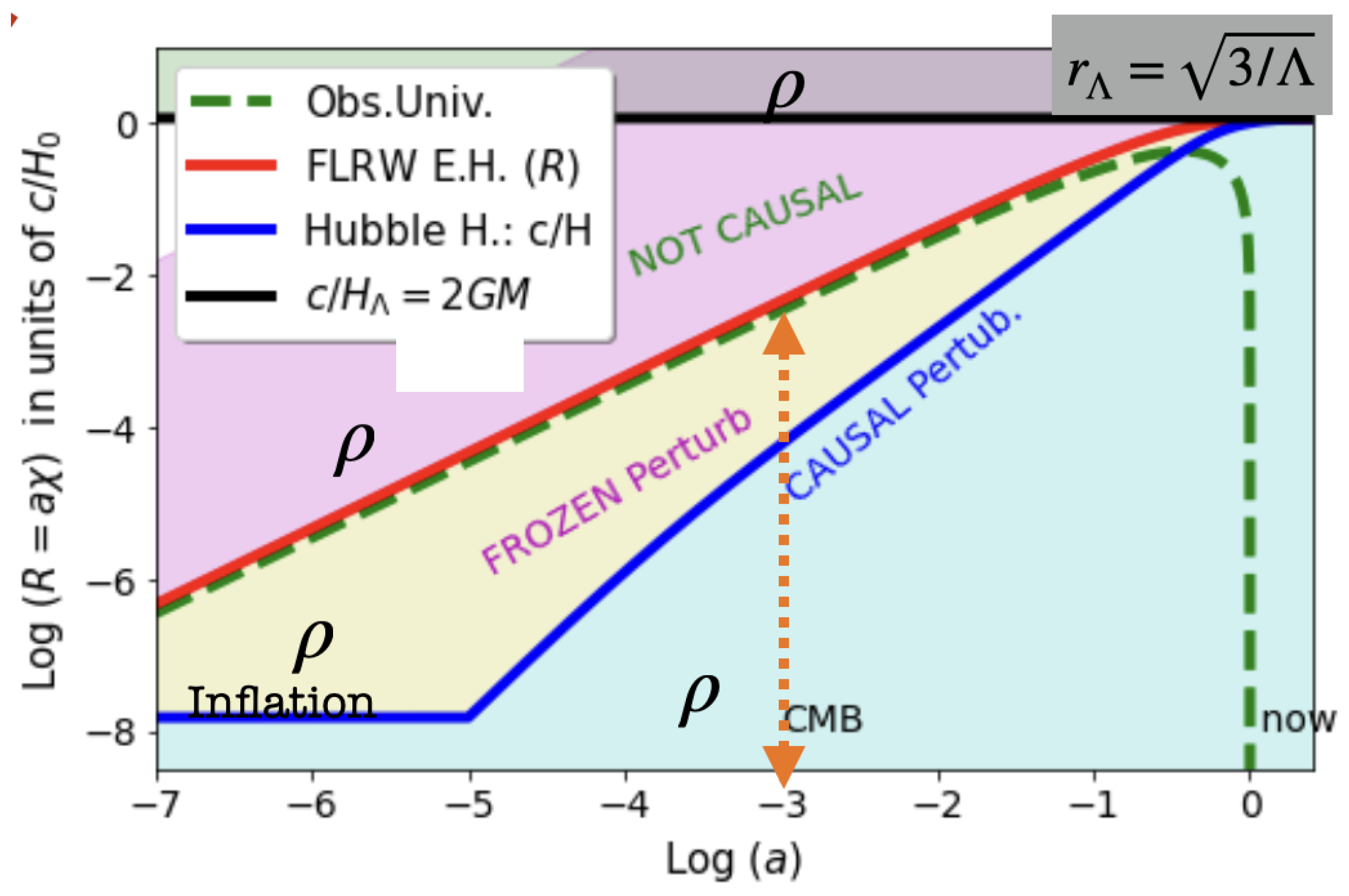
This is illustrated in Figure 4, which also demonstrates how inflation and the horizon problem (i.e., the observation that CMB measurements detect super-horizon frozen perturbations) occurred within . All the observable Universe (green line) is contained inside and we can therefore not measure anything outside.
For we have , so there is no EH. But for we have that (red line in Figure 1). We can then see that corresponds to a causal horizon or boundary term. The analog force behaves like a rubber band between observed galaxies (null events) that prevents them crossing some maximum stretch (i.e. the EH). We can interpret such force as a boundary term that just emerges from the finite speed of light (see the Appendix A).
Figure 4.
Figure 1: Proper coordinate in units of as a function of cosmic time a (scale factor). The Hubble horizon (blue continuous line) is compared to the future Event Horizon (red line) as defined in Eq. 14. Larger radii (magenta shading) represent causally disconnected regions, while smaller ones (yellow shading), created during cosmic inflation, remain dynamically frozen. The full observable universe (dashed green line) encompasses both causal (blue shading) and frozen regions but is bounded by . Compared to Figure 2, which depicts a view at a fixed a using the same color coding. After inflation, begins growing again, and by (present epoch), both and approach (in black).
The FLRW metric with , asymptotically tends to the de-Sitter metric in Eq.4. This form corresponds to a static 4D hyper-sphere of radius . So in this (rest) frame, events can only travel a finite distance within a static 3D surface of the imaginary 4D hyper-sphe The region inside is causally disconnected from the outside. In the context of FLRW framework, this condition corresponds to , where is a radial (space-like) distance. This condition implies that the expansion interpretation is valid only as long as , indicating that it does not make sense for larger values where we cannot transition from to . Essentially, beyond this threshold, the cosmological interpretation of expansion breaks down due to the causal disconnection imposed by the horizon defined at .
As shown in Eq.6, this frame duality can be understood as a Lorentz boost. An observer in the rest frame, sees the moving fluid element contracted by the Lorentz factor . This duality is better understand using our new measures for the expansion rate and cosmic deceleration based on the distance between causal events.
6. Comparison to Data
We show next how to estimate the new measure of cosmic acceleration, , using direct astrophysical observations. As an example consider the Supernovae Ia (SNIa) data as given by the ’Pantheon Sample’ compilation ([11]) consisting on 1048 SNIas between . Each SNIa provides a direct estimate of the luminosity distance at a given measured redshift z. This corresponds to the comoving look-back distance:
so that gives us directly . The second derivative gives us the acceleration:
is given by the model prediction in Eq.14 (arbitrarily fixed at in both data and models). We adopt here the approach presented in [12], who used an empirical fit to the luminosity distance measurements, based on a third-order logarithmic polynomial:
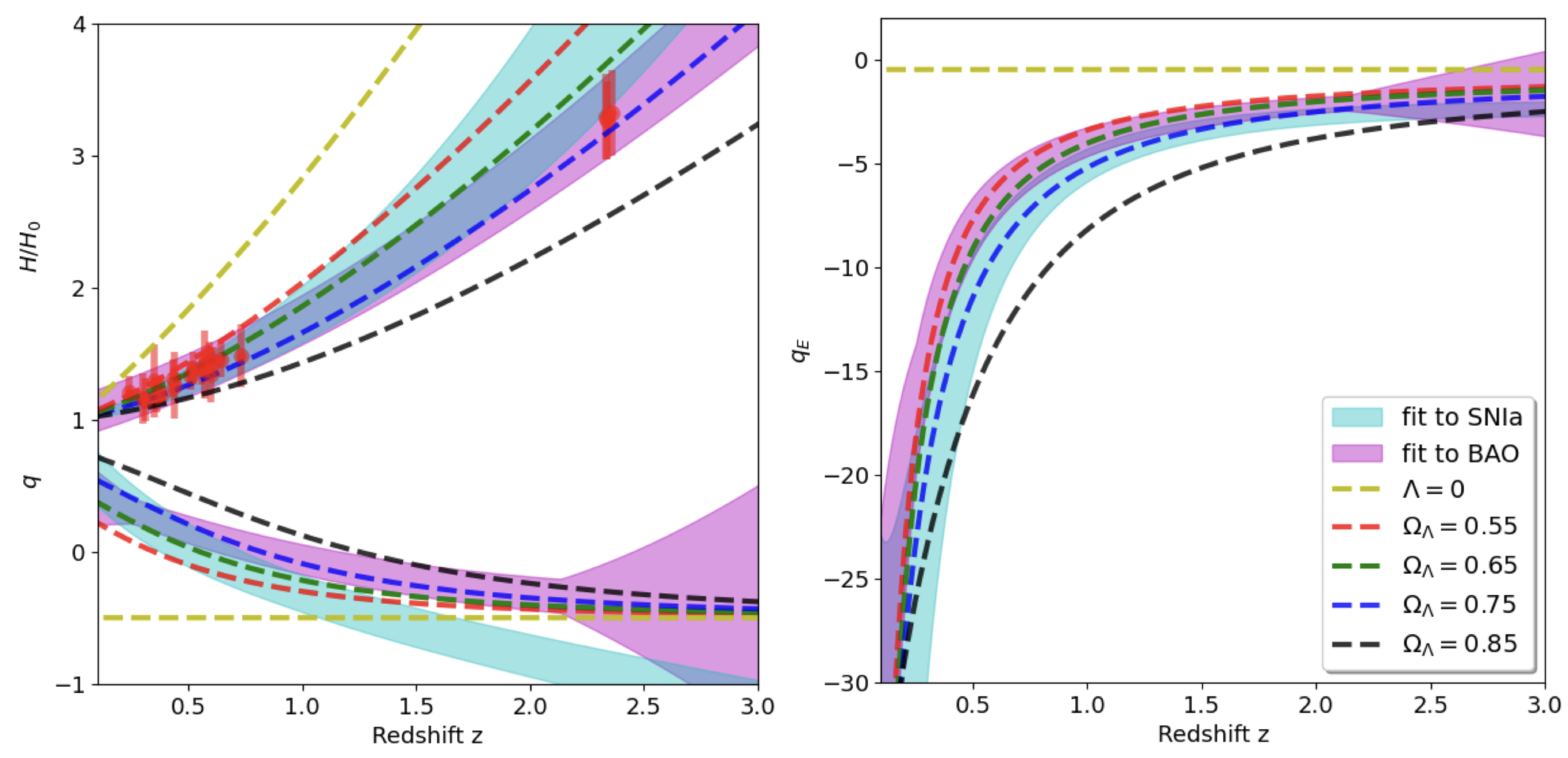
where . [12] find a good fit to: and to the full SNIa ’Pantheon Sample’. We use these values of A and B and its corresponding errors to estimate H, q and using the above relations. Results for H and q are shown as shaded cyan regions in the left panel Figure 5. They are compared to the LCDM predictions in Eq.2 and 3.
There is a very good agreement in for . At , the estimates are also consistent with the predictions. But the detailed evolution with redshift in the SNIa data does not seem to follow any of the model predictions, specially for . The estimates are too steep compare to the different models predictions. If we compare instead the estimates (see right panel of Figure 5) we find a much better agreement with the model predictions. This seems to validate our approach, but it is not clear from this comparison alone if this is caused by the fitting function use in Eq.17.
To test this further we use measurements of the radial BAO data to estimate . Such measurements give us a direct estimate of (as first demonstrated by [13,14]) so they have the advantage over SNIa that we only need to do a first order derivative, to estimate q or :
As an illustration we use measurements presented in Table 2 in [15]. This compilation of is shown as red points with errorbars in the left panel Figure 5. The compilation include values from the clustering of galaxies () and Ly-alpha forest in QSO (). The combination of two separate ranges of redshift allows for a very good measurement of at the intermediate redshift (), where we found the discrepancies in SNIa for q and model comparison (see above). The radial BAO provides a very good constraint on cosmic acceleration, independent of possible calibration errors in or sampling errors (from small area samples). This is something that we can not yet do with the current SNIa data, but will be very interesting to see in the near future with upcoming data from wider and deeper surveys.
We fit a quadratic polynomial to the radial BAO data:
We have checked that the results presented here are very similar if we use a cubic polynomial. In units of Km/s/Mpc, we find , and , with strong covariance between the errors (the cross-correlation coefficient between and is ). The value of is in good agreement with the Planck CMB fit ([16]) but in some tension with the SNIa local calibration: (see [17]). This corresponds to either a local calibration problem (in SNIa, in radial BAO or in both) or a tension in the CDM model at different times or distances (see e.g. [18]). We ignore this normalization problem here and just focus on the evolution of to measure cosmic acceleration q or (which are fairly independent of ).
In the right panel of Figure 5 we show (as shaded regions) the measurements for given by combining Eq.17 with Eq.16 and Eq.19 with Eq.18. The measurements clearly favour models with large negative cosmic event acceleration , which supports our interpretation of as a friction term.
Comparing left and right panels in Figure 5 we see that both q and are rougthly consistent with models with ( or ) in good concordance with in the upper left panel of Figure 5.
Even when the underlying model for q and is the same, note how the measured q and data have different tensions with the model predictions as a function of redshift. In particular, the radial BAO and SNIa data sets show inconsistencies among them for q around . This is a well known tension (see e.g. Figure 17 in [19]). This tension disappears when we use the corresponding estimates for . Thus, data is more consistent with the than with the q description.
One would expect that a perfect realizations of the LCDM model in Eq.2 would produce consistent results in both q and . But deviations from LCDM and systematic effects can produce tensions in data, specially if we use a parametrization, like q, which refers to events that we never observe. The q and parametrization of acceleration are more general than the particular LCDM model and the fact that data prefers is an important indication. Data lives in the light-cone, which corresponds to rather than q. At the difference between a light-cone and space-like separations is very significant and any discrepancies in the data or model will show more pronounced in the q modeling.
We conclude that the data shows some tensions with LCDM predictions (as indicated by q) but confirms that cosmic expansion is clearly decelerating (as indicated by ) so that events are trapped inside an Event Horizon ().
7. Discussion & Conclusion
In our exploration, we’ve demonstrated that the commonly interpreted term, thought to drive cosmic acceleration (as discussed in §2), actually leads to a quicker cosmic deceleration of events compared to the influence of gravity alone (as explained in §4). This explains the origin of the Event Horizon (EH, see §5) that results from an expansion dominated by . It suggests that might not be a new form of vacuum energy ([4,5,6]) but rather a boundary or surface term in the field equations.
The measured in our cosmic expansion behaves analogously to the interior of a Schwarzschild Black Hole (BH), with an identical behavior under the assumption of approximately empty space outside (see [9]). This concept finds support in Figure 2 and Figure 4 because it challenges the notion of how the background density inside and outside can maintain identical values at all times (as assumed in the FLRW metric) without causal connections between these regions.
Additionally, we can conjecture from this notion that the interior dynamics of any other Schwarzschild BH could also be interpreted as having a similar surface term for expanding interior BH solutions. The term thus becomes the mechanism that effectively prevents anything from escaping the BH interior (see [20]).
The Event Horizon measured with (i.e. Eq.14, which is equivalent to the presence of ) also tell us that there is a finite mass trapped within . If we assume that the space outside is approximately empty, such finete mass provides the explanation for the observed and therefore for : i.e. (see [21]).
That is fixed by the total mass of our universe is in good agreement with the physical interpretation presented here that corresponds to a friction (attractive) force that decelerates cosmic events. In the Appendix A we elaborate in this idea and revisit the Newtonian limit to show that corresponds to an additional (attractive) Hooke’s term to the inverse square gravitational law. A rubber band Universe.
Funding
This work was partially supported by grants from Spain Plan Nacional (PGC2018-102021-B-100) and Maria de Maeztu (CEX2020-001058-M) and from European Union LACEGAL 734374 and EWC 776247. IEEC is funded by Generalitat de Catalunya.
Data Availability Statement
No new data are presented.
Conflicts of Interest
The author declares no conflict of interest.
Appendix A. Newtonian and Hookeonian Limits
When we talk about classical forces we are making an analogy to Newton’s law to gain some intuition on the physical problem. This is why we study next the role of in the non-relativistic limit. Consider the geodesic acceleration defined from the geodesic deviation equation (see [22]):
where is the separation vector between neighbouring geodesics and is the tangent vector to the geodesic. For an observer following the trajectory of the geodesic and :
and we can choose the separation vector to be the spatial coordinate. The spatial divergence of is then:
This equation is always valid for a comoving observer (see Eq.6.105 in [22]). Newtonian gravity is reproduced for the case of non-relativistic matter (). The gravitational force (without ) is always attractive for (because and therefore ) but it can be repulsive when . For example, in the case of pure vacuum energy with , we have and a repulsive gravitational force . The covariant version of Eq.A3 is the relativistic version of Poisson’s Equation (see also [23,24]):
The solution to these equations is given by an integral over the usual propagators or retarded Green functions which account for causality.
This is also the Raychaudhuri equation for a shear-free, non-rotating fluid where and is the 4-velocity:
The above equation is purely geometric: it describes the evolution in proper time of the dilatation coefficient of a bundle of nearby geodesics. Note that without , the acceleration is always negative unless which is what we call DE today. This is degenerate with the term for constant , so we can argue that is a particular case of DE (but it can also be interpreted as a modify gravity term).
In the non-relativistic limit we see from Eq.A3 that indeed corresponds to a repulsive force that dominates at large distances. For point like source:
and acceleration can only be caused by (see also [23,25]). Note how the linear term has the wrong sing compare to Hooke’s law. It actually makes little sense to take the strict non-relativistic limit in Cosmology because in that limit, photons from different times will reach us instantly as in Eq.7. To make sense of observations we need to take into account the intrinsically relativistic effect that the speed of propagation is finite (). This corresponds to an additional term to the covariant acceleration which results in Eq.13. So besides gravitational deceleration, there is also a friction term proportional to H, caused by the expansion itself:
So that the corresponding point like source is:
The negative friction term is always larger than the positive term and asymptotically cancels it. This changes the sign of our interpretation of the role of in terms of classical forces. The additional term has now the standard sign of Hooke’s law in the above equation, so the effect of the term could just be interpreted as a rubber band like force that prevents the crossing of the EH. We could summarize this as: accelerates the 3D coordinate spatial expansion in and this causes an additional deceleration in the expansion of events which results in an EH or a trapped surface.
References
- de Boer, J.; Dittrich, B.; Eichhorn, A.; Giddings, S.B.; Gielen, S.; Liberati, S.; Livine, E.R.; Oriti, D.; Papadodimas, K.; Pereira, A.D.; Sakellariadou, M.; Surya, S.; Verlinde, H. Frontiers of Quantum Gravity: shared challenges, converging directions. e-prints 2022, p. arXiv:2207.10618.
- DES Collaboration. DES Year 3 results: Cosmological constraints from galaxy clustering and weak lensing. PRD 2022, 105, 023520. [Google Scholar] [CrossRef]
- Huterer, D.; Turner, M.S. Prospects for probing the dark energy via supernova distance measurements. PRD 1999, 60, 081301. [Google Scholar] [CrossRef]
- Weinberg, S. The cosmological constant problem. Reviews of Modern Physics 1989, 61, 1–23. [Google Scholar] [CrossRef]
- Carroll, S.M.; Press, W.H.; Turner, E.L. The cosmological constant. ARAA 1992, 30, 499–542. [Google Scholar] [CrossRef]
- Peebles, P.J.; Ratra, B. The cosmological constant and dark energy. Reviews of Modern Physics 2003, 75, 559–606. [Google Scholar] [CrossRef]
- Lanczos, K. Bemerkung zur de Sitterschen Welt. Phys.Z. 1922, 23, 539–543. [Google Scholar]
- Mitra, A. Interpretational conflicts between the static and non-static forms of the de Sitter metric. Nature Sci. Reports 2012, 2, 923. [Google Scholar] [CrossRef] [PubMed]
- Gaztañaga, E. The Black Hole Universe, Part I. Symmetry 2022, 14, 1849. [Google Scholar] [CrossRef]
- Ellis, G.F.R.; Rothman, T. Lost horizons. American Journal of Physics 1993, 61, 883–893. [Google Scholar] [CrossRef]
- Scolnic, D.M.; Jones, D.O.; Rest, A.; Pan, Y.C.; Chornock, R.; Foley, R.J.; Huber, M.E.; Kessler, R.; Narayan, G.; Riess, A.G.; Rodney, S.; Berger, E.; Brout, D.J.; Challis, P.J.; Drout, M.; Finkbeiner, D.; Lunnan, R.; Kirshner, R.P.; Sanders, N.E.; Schlafly, E.; Smartt, S.; Stubbs, C.W.; Tonry, J.; Wood-Vasey, W.M.; Foley, M.; Hand, J.; Johnson, E.; Burgett, W.S.; Chambers, K.C.; Draper, P.W.; Hodapp, K.W.; Kaiser, N.; Kudritzki, R.P.; Magnier, E.A.; Metcalfe, N.; Bresolin, F.; Gall, E.; Kotak, R.; McCrum, M.; Smith, K.W. The Complete Light-curve Sample of Spectroscopically Confirmed SNe Ia from Pan-STARRS1 and Cosmological Constraints from the Combined Pantheon Sample. ApJ 2018, 859, 101. [Google Scholar] [CrossRef]
- Liu, Y.; Cao, S.; Biesiada, M.; Lian, Y.; Liu, X.; Zhang, Y. Measuring the Speed of Light with Updated Hubble Diagram of High-redshift Standard Candles. ApJ 2023, 949, 57. [Google Scholar] [CrossRef]
- Gaztañaga, E.; Miquel, R.; Sánchez, E. First Cosmological Constraints on Dark Energy from the Radial Baryon Acoustic Scale. Phy.Rev.Lett. 2009, 103, 091302. [Google Scholar] [CrossRef]
- Gaztañaga, E.; Cabré, A.; Hui, L. Clustering of luminous red galaxies - IV. Baryon acoustic peak in the line-of-sight direction and a direct measurement of H(z). MNRAS 2009, 399, 1663–1680. [Google Scholar] [CrossRef]
- Niu, J.; Chen, Y.; Zhang, T.J. Reconstruction of the dark energy scalar field potential by Gaussian process. e-prints 2023, p. arXiv:2305.04752.
- Planck Collaboration. Planck 2018 results. VI. Cosmological parameters. A&A 2020, 641, A6. [Google Scholar]
- Riess, A.G. The expansion of the Universe is faster than expected. Nature Reviews Physics 2019, 2, 10–12. [Google Scholar] [CrossRef]
- Abdalla, E.; et al. Cosmology intertwined: A review of the particle physics, astrophysics, and cosmology associated with the cosmological tensions and anomalies. JHEA 2022, 34, 49–211. [Google Scholar]
- Bautista, J.; et al. Measurement of baryon acoustic oscillation correlations at z = 2.3 with SDSS DR12 Lyα-Forests. A& A 2017, 603, A12. [Google Scholar]
- Gaztañaga, E. Do White Holes Exist? Universe 2023, 9, 194. [Google Scholar] [CrossRef]
- Gaztañaga, E. The mass of our observable Universe. MNRAS 2023, 521, L59–L63. [Google Scholar] [CrossRef]
- Padmanabhan, T. Gravitation, Cambridge U. Press; 2010.
- Gaztañaga, E. The size of our causal Universe. MNRAS 2020, 494, 2766–2772. [Google Scholar] [CrossRef]
- Gaztañaga, E. The cosmological constant as a zero action boundary. MNRAS 2021, 502, 436–444. [Google Scholar] [CrossRef]
- Calder, L.; Lahav, O. Dark energy: back to Newton? Astronomy & Geophysics 2008, 49, 1–13. [Google Scholar]
Figure 1.
Log of cosmic expansion rate (continuous lines) and acceleration (dashed lines) as a function of time (log scale factor a) for . The black lines correspond to the usual interpretation in terms of 3D spatial coordinates: H and q. The blue lines show the corresponding results for the measurement in terms of 4D events: and . Without both are equivalent. Gravity decelerates the expansion until it asymptotically brings it to a halt (, with an EH: ). The effect of according to the coordinate interpretation is to accelerate the expansion. While according to the proper distance R, it decelerates the expansion even further and brings it to an early halt: and at a finite horizon . This additional deceleration is caused by the friction term: in Eq.12-13 (dashed-dot red line).
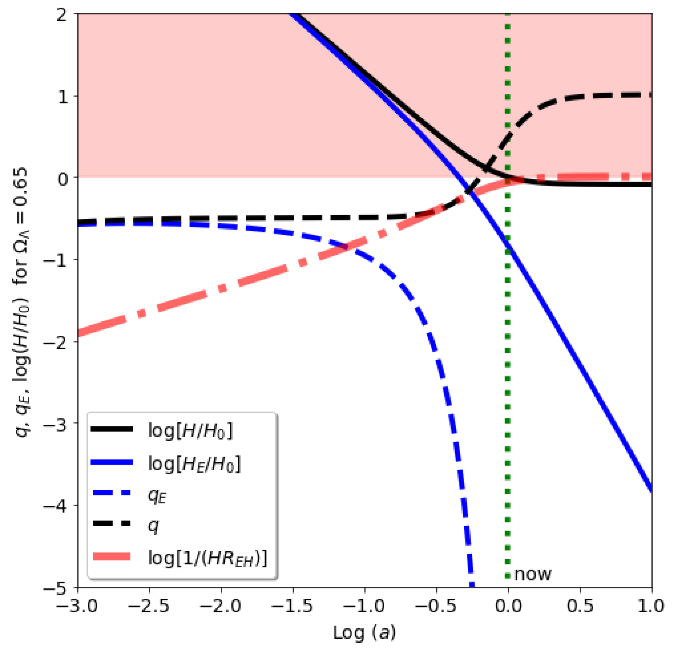
Figure 2.
The left panel shows a spatial representation of FLRW metric in Eq.6 as a 2D metric (magenta plane) in polar coordinates (one angle is fixed) embedded in 3D flat space (where z in the plot corresponds to an extra dimension to illustrate the geometry). De-Sitter metric corresponds to the outer sphere , while the FLRW metric is the blue sphere of radius asymptotycaly expanding into . The yellow/blue region shows the super/sub horizon causal regions. The right panel shows the same 2D plane faced on, where we have also included (in red) the FLRW event Horizon R, discussed in §5 and Figure 4. Scales can never be reached from inside. Because is causally disconnected from the inside, this region should have the Schwarzschild metric with if fully empty.
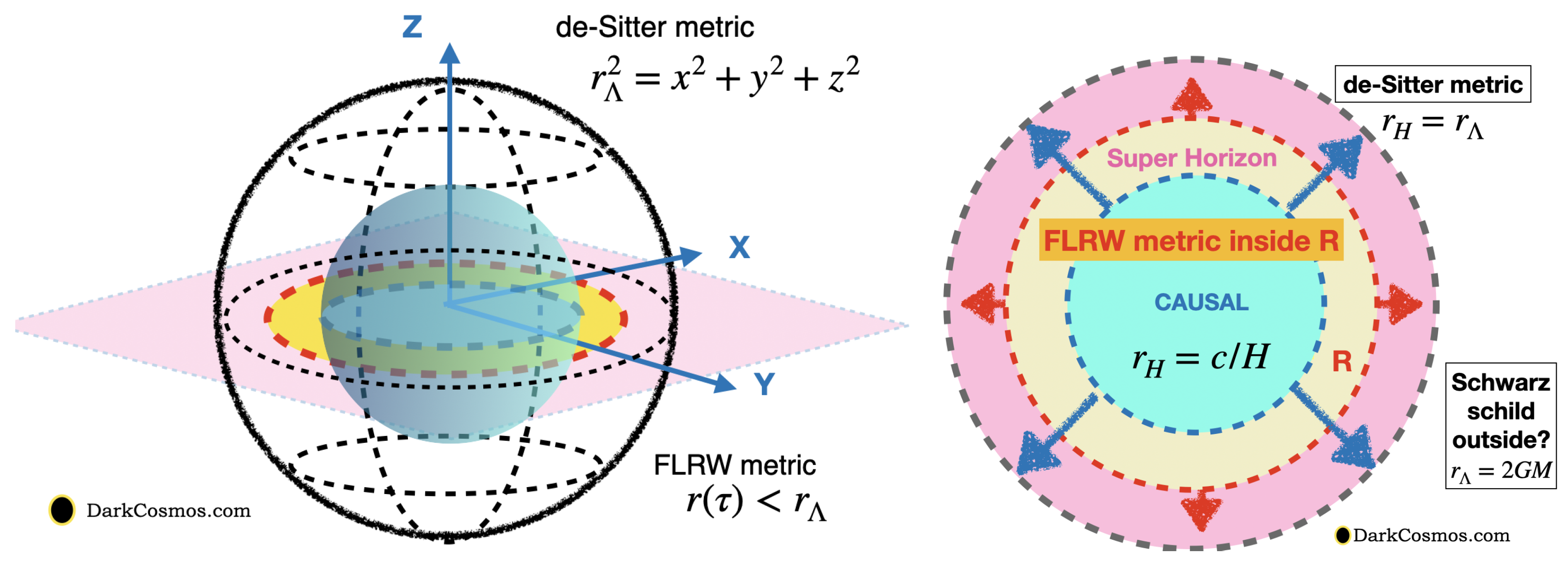
Figure 3.
Comparison of different distances in the FLRW metric of Eq.1 between an observed event (at emission) at coordinates and the corresponding null event (at reception) somewhere in its future . The space-like distance in Eq.7, along the horizontal axis, is the one commonly used to define cosmic acceleration. It expands as , but is not causally connected. The distance in Eq.8, along the vertical axis, is the time-like distance traveled by light, but is independent of cosmic expansion . The event distance R in Eq.9 corresponds to the proper distance in the light-cone between the two events and is the one we should used to properly interprete cosmic expansion.
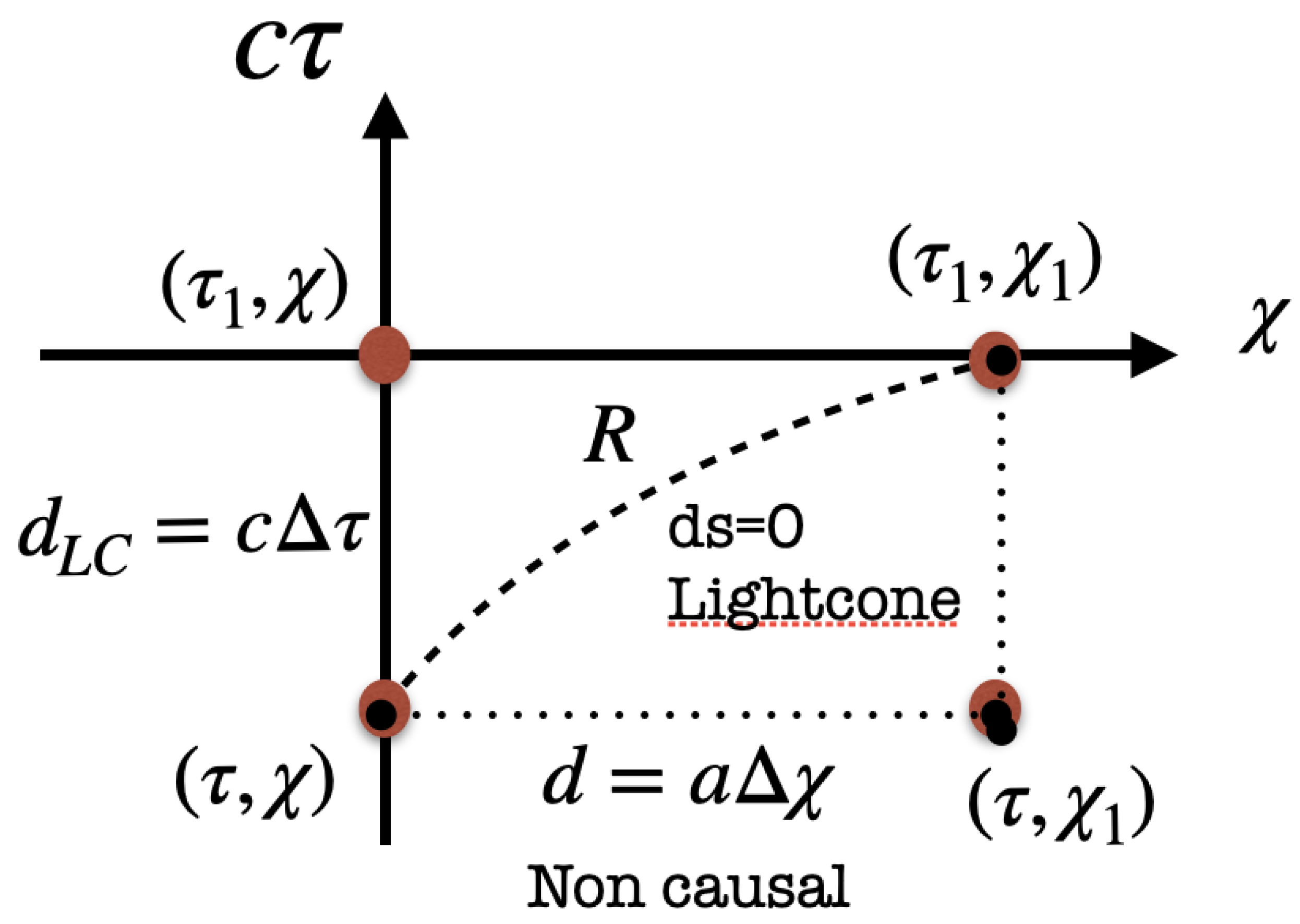
Figure 5.
Expansion rate (upper left panel), cosmic acceleration q (lower left panel) and event acceleration (right panel). Shaded areas correspond to a polynomial fit with region in a sample of SNIa (cyan) and radial BAO measurements (magenta). Dashed lines show the corresponding LCDM predictions for different values of as labeled.
Disclaimer/Publisher’s Note: The statements, opinions and data contained in all publications are solely those of the individual author(s) and contributor(s) and not of MDPI and/or the editor(s). MDPI and/or the editor(s) disclaim responsibility for any injury to people or property resulting from any ideas, methods, instructions or products referred to in the content. |
© 2024 by the authors. Licensee MDPI, Basel, Switzerland. This article is an open access article distributed under the terms and conditions of the Creative Commons Attribution (CC BY) license (http://creativecommons.org/licenses/by/4.0/).
Copyright: This open access article is published under a Creative Commons CC BY 4.0 license, which permit the free download, distribution, and reuse, provided that the author and preprint are cited in any reuse.


