Submitted:
12 September 2023
Posted:
13 September 2023
You are already at the latest version
Abstract
In the present work we consider two modified Chevallier-Polarski-Linder (CPL) models in the background of homogeneous and isotropic FLRW space-time, namely (i) the generalized CPL model (Model I) and (ii) the logarithmic form of the the equation of state for the dark energy. From the observational data sets ((Pantheon+)+BAO+HST), we find that at the present epoch (redshift $z=0$), the equation of state for the dark energy converges almost at the same value $\omega_{fld}\approx -0.86$ and the variation of $\omega_{fld}(z)$ with respect to the redshift parameter is very small for both models.
we also find that the present value of the Hubble parameter $H_0$ is almost same for both the models.
Finally, we compare the models in the light of Akaike, Bayesian Information Criterion (BIC) and Bayesian Evidence. However, we find that Model II is better compared to the Model I from the estimated value of the deceleration parameter.
Keywords:
dark energy
; CPL model
; observational analysis
1. Introduction
Several independent observations, namely Type Ia supernovae (SN Ia) [1,2], cosmic microwave background (CMB) [3,4,5,6], Baryonic Acoustic Oscillation [7,8], Wilkinson Microwave Anisotropy Probe (WMAP) [9] established for the last two decades that our universe is going through an accelerating expansion phase in the present time. This acceleration started at recent past [10,11] and this phase is known as late-time acceleration in cosmology. However, the cause of this acceleration is unknown. In order to address this issue, cosmologists trying to search in two distinct paths. Firstly, Modifying the gravity theory [12,13,14,15,16,17,18,19], and secondly, introducing some unknown kind of exotic matter, namely, dark energy, which have large negative pressure [20,21,22,23,24,25]. However, after the incredible success of Einstein gravity theory through the gravity wave detection [26,27], cosmologists are more inclined to the second option.
If one assumes our universe is filled with barotropic fluid, then the accelerating phase indicates the equation of state for dark energy is . The CDM model () is the best simplest model which supports the observation. However, it has potential drawback which is known as cosmological constant problem [28,29,30,31]. There are also several studies where the equation of state for the dark energy is considered as a function of redshift parameter z, for example, phantom fields [32,33,34], tachyons [35], quintessence[36,37,38], k-essence model [39,40], etc.
If the equation of state for the dark energy is considered to be an arbitrary function of redshift parameter z, then one needs infinite number of datasets to constrain the model parameter as an unknown function can be expand in terms of infinite Taylor (or, Laurent) series, which is practically impossible. Therefore, cosmologists attempt with considering finite number of parameters in the equation of state for the dark energy. One of the popular models is Chevallier-Polarski-Linder (CPL) model which has two parameters in the equation state having explicit form as [41,42]
where and are constant. The notable feature for the model is that it is a well behaved and bounded function at high redshift and linear in z at low redshift.
In the present work, we shall choose two possible modifications of this CPL equation of state and examined them from the observational view point. The plan of the paper is as follows: In Section 2, basic equations of non-interacting DM and DE Friedmann-Lemaitre-Robertson-Walker (FLRW) cosmology has been presented and two specific equation of state of DE has been introduced. Section 3, deals with the numerical investigation of these models with the observational data, while Section 4, a comparison study of these models has been shown on the basis of Akaike, Bayesian Information criteria and Bayesian evidence. The paper ends with a conclusion in Section 5.
2. Friedmann-Lemaitre-Robertson-Walker Cosmology
Now, considering the spatially flat Friedmann-Lemaitre-Robertson-Walker (FLRW) space-time having the line element
the Friedmann equations take the form
where is the scale factor, and is the Hubble parameter. The energy conservation equations of individual component can be expressed as
If one assumes the equation of state for matter component is , the energy density of the matter component can be obtained as
Here, we have considered matter component as dust particle , so . For the dark energy part, we have assumed equation of state parameter varies with the redshift parameter z, then the energy density can be expressed as
where is the present value of the scale factor and it is considered to be and are integration constant. Thus the Hubble parameter H cane expressed as
where and are the present value of the Hubble parameter , matter density and the dark energy density , respectively. Therefore, .
For the dark energy sector, we have considered here two variable of equation of state which are following:
2.1. Model I:
2.2. Model II:
where and are constants. We may emphasize here that the model I is nothing but a generalized form of the CPL model. For , it reduces to CPL model. At low redshift both the models are linear in z. However, at high redshift, for model I, whereas for model II, .
3. Numerical Analysis and Observational constraints
In this section, our goal here is to constrain the cosmological parameters analyzing the observational data sets. In oder to include the dark energy sector as a fluid, we have modified the public version of the CLASS Boltzmann code. The MCMC code Montepython3.5 [43] has been used to estimate the relevant cosmological model parameters.
For the statistical inference, we use the cosmological datasets (Pantheon+ [44], BAO (BOSS DR12 [7], SMALLZ - 2014 [8]) with the latest BAO dataset which spanning the redshift range [45,46,47,48,49] and HST [50]) and a PLANCK18 [51] prior has been imposed. We have made the choice of flat priors on the base cosmological parameters as follows: the baryon density ; cold dark matter density ; Hubble parameter , where . A wide range of flat prior has been chosen for , , and M is the nuisance parameter.
Using the cosmological data sets, we run MCMC until the Gelman- Rubin convergence criterion is reached and we have plotted the posterior distribution for the model I and model II in the Figure 1 and Figure 2, respectively. The corresponding best-fit and mean values are enlisted in Table 1. One can see here that for both models, the best-fit value of is almost same , the present value of the equation of state converges almost at same point. One can also observed that is close to zero for both the models. It means the variation of equation of state for the dark energy with respect to the redshift parameter z is small as shown in the sub-Figure-(a) of Figure 3. We also note that the parameter p can not be constrained for Model I. However, for Model II, it can be constrained and there is also a lower bound on p. In order to understand which model is more preferable, we discuss Akaike, Bayesian Information Criterion (BIC) and Bayesian Evidence in the next section.
One can understand the cosmological models from the different variables like Hubble parameter , deceleration parameter , jerk parameter which are all derived from the derivatives of the scale factor. Using the best fit value of the cosmological parameters of the different models inferred from the cosmological datasets, we have plotted the Hubble parameter with respect the redshift z in sub-Figure (b) of Figure 3. One can see here that is monotonically increasing with z and it is almost same for both the models. We also plotted the deceleration parameter in the sub-Figure (c) of Figure 3, which is defined as [52]
Here it is observed that the Model I has gone through from deceleration to acceleration phase at whereas Model II at . However, the present value of deceleration parameter is quite distinct, namely for Model I that implies (from Eq. 8) that which does not support observation but for Model II which supports the observation. We have also plotted the jerk parameter in the sub-Figure (d) of Figure 3, which is defined as [53,54]
Here, one can see that at higher z it converges to for both models.
4. Information Criteria and Model Comparison
In order to make a comparison between the models, here we apply the well known Akaike Information Criterion (AIC) [55] and the Bayesian Information Criterion (BIC) [56]. This allows us to analyze which model best fits the observational data. Based on the information theory, AIC is an estimator of the Kullback-Leibler information with the property of asymptotically unbiasedness. Under the standard Gaussian error assumptions, the expression of AIC reads as [57,58,59]
where is the maximum likelihood of the datasets, is the total data points and k is the number of parameters of the model. For large number of data points , it reduces to . The AIC gives goodness of fit through the maximum likelihood. However, the additional term of the AIC acts as a penalty for models which have a large number of parameters. Whereas, the BIC is defined as [60,61]
It is clearly seen that the penalty for BIC is higher than that of AIC. In general, the model having lower values of AIC and BIC corresponds to the model that best fits the data.
4.1. The Bayesian Evidence
For the given dataset D, the posterior probability distribution of a model is related by the Likelihood function and prior is related by Bayes’ theorem
where is the parameter of the model and the normalization constant E is called the Bayesian evidence which is given by
where is the parameter space under the model . The ratio of the Bayesian evidences for the two competing models is given by
which is known as the Bayes factor. In order to determine the preference for one model over another, we used Jeffrey’s scale. According to it the decisive condition is summarized in the Table 3 [62].
We have computed Bayesian evidence using the publicly available code MCEvidence [63] and the results are enlisted in the Table 2. From the table, it is seen that in the context of AIC and BIC, both models are very close to each other and from the Bayesian Evidence, the value . Therefore, on the basis of these statistical analysis we can not make any comment on which model is more preferable.
5. Conclusion
A detailed study has been done for the two modified CPL models where the dark energy is considered as a perfect fluid and the equation of state is chosen as the generalized form of CPL model(Model I) and logarithmic form (Model II). The parameters involved in these two models are estimated from the observation data data sets (Pantheon+ [44], BAO [7,8,45,46,47,48,49] and HST [50]) with prior from PLANCK18 data set [51].
From the observational analysis using the data set I, it is found that the parameter p can not be constrained for the model I. However, for model II it can be constrained and there is a lower bound on it. For both the models, the parameter converges at and is close to zero for both models which indicates that the equation of state varies very slowly. We also notice that the Hubble parameter is very close to each other.
We have also plotted the deceleration parameter which goes from deceleration to acceleartion phase near for the model I and near for model II. We have also plotted jerk parameter where one can see that at higher z it converges to for both models. Finally, we have compared the models analyzing AIC, BIC and Bayesian Evidence. Here we have seen that the value of AIC and BIC are almost same and . Therefore, it is very hard to find the best model between them. Though both the CPL modified paramatrization models are identical from the observed dataset considered in the paper but all the parameters in model II can be constrained but it is not possible for model I. Moreover, the present value of deceleration parameter for Model I which does not support observation. Therefore, we may conclude that Model II is better compared to the Model I.
Acknowledgments
The authors would like to thank Nandan Roy and Supriya Pan for helping to run Montepython. G.S. acknowledges UGC for Dr. D.S. Kothari Postdoctoral Fellowship (No.F.4-2/2006 (BSR)/PH/19-20/0104) and S.C. thanks FIST program of DST, Department of Mathematics, JU (SR/FST/MS-II/2021/101(C)).
References
- Conley et al. Supernova constraints and systematic uncertainties from the first three years of the supernova legacy survey*. The Astrophysical Journal Supplement Series, 192(1):1, dec 2010.
- James Guillochon, Jerod Parrent, Luke Zoltan Kelley, and Raffaella Margutti. An open catalog for supernova data. The Astrophysical Journal, 835(1):64, jan 2017.
- P. A. R. Ade et al. Planck 2013 results. I. Overview of products and scientific results. Astron. Astrophys., 571:A1, 2014.
- R. Adam et al. Planck 2015 results. I. Overview of products and scientific results. Astron. Astrophys., 594:A1, 2016.
- P. A. R. Ade et al. Planck 2015 results. XIII. Cosmological parameters. Astron. Astrophys., 594:A13, 2016.
- N. Aghanim et al. Planck 2015 results. XI. CMB power spectra, likelihoods, and robustness of parameters. Astron. Astrophys., 594:A11, 2016.
- Shadab Alam, Metin Ata, Stephen Bailey, Florian Beutler, Dmitry Bizyaev, Jonathan A. Blazek, Adam S. Bolton, Joel R. Brownstein, Angela Burden, and Chuang et al. The clustering of galaxies in the completed sdss-iii baryon oscillation spectroscopic survey: cosmological analysis of the dr12 galaxy sample. Monthly Notices of the Royal Astronomical Society, 470(3):2617–2652, Mar 2017.
- Ashley J. Ross, Lado Samushia, Cullan Howlett, Will J. Percival, Angela Burden, and Marc Manera. The clustering of the sdss dr7 main galaxy sample – i. a 4 per cent distance measure at z = 0.15. Monthly Notices of the Royal Astronomical Society, 449(1):835–847, Mar 2015.
- G. Hinshaw, D. Larson, E. Komatsu, D. N. Spergel, C. L. Bennett, J. Dunkley, M. R. Nolta, M. Halpern, R. S. Hill, N. Odegard, L. Page, K. M. Smith, J. L. Weiland, B. Gold, N. Jarosik, A. Kogut, M. Limon, S. S. Meyer, G. S. Tucker, E. Wollack, and E. L. Wright. Nine-year wilkinson microwave anisotropy probe (wmap) observations: Cosmological parameter results. The Astrophysical Journal Supplement Series, 208(2):19, sep 2013.
- David H. Weinberg, Michael J. Mortonson, Daniel J. Eisenstein, Christopher Hirata, Adam G. Riess, and Eduardo Rozo. Observational probes of cosmic acceleration. Physics Reports, 530(2):87–255, 2013. Observational Probes of Cosmic Acceleration.
- Olga Avsajanishvili, Lado Samushia, Natalia A. Arkhipova, and Tina Kahniashvili. Testing Dark Energy Models through Large Scale Structure.
- Timothy Clifton, Pedro G. Ferreira, Antonio Padilla, and Constantinos Skordis. Modified gravity and cosmology. Physics Reports, 513(1):1–189, 2012. Modified Gravity and Cosmology.
- Timothy Clifton, Pedro G. Ferreira, Antonio Padilla, and Constantinos Skordis. Modified Gravity and Cosmology. Phys. Rept. 2012; 513, 1–189.
- Emmanuel, N. Saridakis et al. Modified Gravity and Cosmology: An Update by the CANTATA Network. 5 2021.
- Shin’ichi Nojiri and Sergei, D. Odintsov. Modified f(R) gravity consistent with realistic cosmology: From matter dominated epoch to dark energy universe. Phys. Rev. D, 2006; 74, 086005. [Google Scholar]
- Eric V. Linder. Einstein’s Other Gravity and the Acceleration of the Universe. Phys. Rev. D, 81:127301, 2010. [Erratum: Phys.Rev.D 82, 109902 (2010)].
- Tiberiu Harko, Francisco S. N. Lobo, G. Otalora, and Emmanuel N. Saridakis. f(T,T) gravity and cosmology. JCAP, 2014; 12, 021.
- Salvatore Capozziello and Mariafelicia De Laurentis. Extended Theories of Gravity. Phys. Rept. 2011; 509, 167–321.
- Antonio De Felice and Shinji Tsujikawa. f(R) theories. Living Rev. Rel. 2010; 13, 3.
- Varun Sahni and Alexei Starobinsky. Reconstructing Dark Energy. Int. J. Mod. Phys. D, 2006; 15, 2105–2132.
- H. K. Jassal, J. S. H. K. Jassal, J. S. Bagla, and T. Padmanabhan. WMAP constraints on low redshift evolution of dark energy. Mon. Not. Roy. Astron. Soc. 2005; 356, L11–L16. [Google Scholar]
- Yun Wang, Veselin Kostov, Katherine Freese, Joshua A. Frieman, and Paolo Gondolo. Probing the evolution of the dark energy density with future supernova surveys. JCAP, 2004; 12, 003.
- Seokcheon Lee. Constraints on the dark energy equation of state from the separation of CMB peaks and the evolution of alpha. Phys. Rev. D, 2005; 71, 123528.
- Edvard Mörtsell and Suhail Dhawan. Does the Hubble constant tension call for new physics? JCAP, 2018; 09, 025.
- Weiqiang Yang, Supriya Pan, Eleonora Di Valentino, Emmanuel N. Saridakis, and Subenoy Chakraborty. Observational constraints on one-parameter dynamical dark-energy parametrizations and the H0 tension. Phys. Rev. D, 2019; 99(4), 043543.
- B. P. Abbott et al. Observation of Gravitational Waves from a Binary Black Hole Merger. Phys. Rev. Lett. 2016; 116(6), 061102.
- B. P. Abbott et al. Tests of general relativity with GW150914. Phys. Rev. Lett., 116(22):221101, 2016. [Erratum: Phys.Rev.Lett. 121, 129902 (2018)].
- P. J. E. Peebles and Bharat Ratra. The Cosmological Constant and Dark Energy. Rev. Mod. Phys. 2003; 75, 559–606.
- J. S. Farnes. A unifying theory of dark energy and dark matter: Negative masses and matter creation within a modified ΛCDM framework. Astron. Astrophys. 2018; 2018, A92.
- G. Efstathiou, W. J. Sutherland, and S. J. Maddox. The cosmological constant and cold dark matter. Nature, 1990; 348, 705–707.
- M. Membrado and A. F. Pacheco. Effects of the cosmological constant on cold dark matter clusters. Astron. Astrophys. 2014; 567, A37.
- R. R. Caldwell. A Phantom menace? Phys. Lett. B, 2002; 545, 23–29.
- Jian-gang Hao and Xin-zhou Li. Phantom with born-infeld-type lagrangian. Phys. Rev. D, 68:043501, Aug 2003.
- G. W. Gibbons. Phantom matter and the cosmological constant. 2 200.
- T. Padmanabhan. Accelerated expansion of the universe driven by tachyonic matter. Phys. Rev. D, 66:021301, 2002.
- S. Sen and T. R. Seshadri. Selfinteracting Brans-Dicke cosmology and quintessence. Int. J. Mod. Phys. D, 2003; 12, 445–460.
- Claudio Rubano and Paolo Scudellaro. On some exponential potentials for a cosmological scalar field as quintessence. Gen. Rel. Grav. 2002; 34, 307–328.
- Sidney, A. Bludman and M. Roos. Quintessence cosmology and the cosmic coincidence. Phys. Rev. D, 2002; 65, 043503. [Google Scholar]
- Luis, P. Chimento and Alexander Feinstein. Power - law expansion in k-essence cosmology. Mod. Phys. Lett. A, 2004; 19, 761–768. [Google Scholar]
- Robert, J. Scherrer. Purely kinetic k essence as unified dark matter. Phys. Rev. Lett. 2004; 93, 011301. [Google Scholar]
- Michel Chevallier and David Polarski. Accelerating universes with scaling dark matter. Int. J. Mod. Phys. D, 2001; 10, 213–224.
- Eric, V. Linder. Exploring the expansion history of the universe. Phys. Rev. Lett. 2003; 90, 091301. [Google Scholar]
- Thejs Brinckmann and Julien Lesgourgues. MontePython 3: boosted MCMC sampler and other features. Phys. Dark Univ. 2019; 24, 100260.
- et al. The Pantheon+ Analysis: The Full Data Set and Light-curve Release. Astrophys. J. 2022; 938(2), 113. [Google Scholar]
- Hector Gil-Marin et al. The Completed SDSS-IV extended Baryon Oscillation Spectroscopic Survey: measurement of the BAO and growth rate of structure of the luminous red galaxy sample from the anisotropic power spectrum between redshifts 0.6 and 1.0. Mon. Not. Roy. Astron. Soc. 2020; 498(2), 2492–2531.
- X. D. Jia, J. P. X. D. Jia, J. P. Hu, and F. Y. Wang. Evidence of a decreasing trend for the Hubble constant. Astron. Astrophys. 2023; 674, A45. [Google Scholar]
- Paul Carter, Florian Beutler, Will J Percival, Chris Blake, Jun Koda, and Ashley J Ross. Low redshift baryon acoustic oscillation measurement from the reconstructed 6-degree field galaxy survey. Monthly Notices of the Royal Astronomical Society, 2018; 481(2), 2371–2383.
- Julian, E. Bautista et al. The Completed SDSS-IV extended Baryon Oscillation Spectroscopic Survey: measurement of the BAO and growth rate of structure of the luminous red galaxy sample from the anisotropic correlation function between redshifts 0.6 and 1. Mon. Not. Roy. Astron. Soc. 2020; 500(1), 736–762. [Google Scholar]
- Richard Neveux et al. The completed SDSS-IV extended Baryon Oscillation Spectroscopic Survey: BAO and RSD measurements from the anisotropic power spectrum of the quasar sample between redshift 0.8 and 2.2. Mon. Not. Roy. Astron. Soc. 2020; 499(1), 210–229.
- Adam, G. Riess, Lucas Macri, Stefano Casertano, Hubert Lampeitl, Henry C. Ferguson, Alexei V. Filippenko, Saurabh W. Jha, Weidong Li, and Ryan Chornock. A 3% SOLUTION: DETERMINATION OF THE HUBBLE CONSTANT WITH THEHUBBLE SPACE TELESCOPEAND WIDE FIELD CAMERA 3. The Astrophysical Journal, 2011; 730(2), 119. [Google Scholar]
- N. Aghanim et al. Planck 2018 results. VI. Cosmological parameters. Astron. Astrophys., 641:A6, 2020. [Erratum: Astron.Astrophys. 652, C4 (2021)].
- Gopal Sardar, Akash Bose, and Subenoy Chakraborty. Observational constraints on f(R, T) gravity with f(R,T)=R+h(T). Eur. Phys. J. C, 2023; 83(1), 41.
- Purba Mukherjee and Narayan Banerjee. Non-parametric reconstruction of the cosmological jerk parameter. Eur. Phys. J. C, 2021; 81(1), 36.
- Abdulla Al Mamon and Kazuharu Bamba. Observational constraints on the jerk parameter with the data of the Hubble parameter. Eur. Phys. J. C, 2018; 78(10), 862.
- H. Akaike. A new look at the statistical model identification. IEEE Transactions on Automatic Control, 1974; 19(6), 716–723.
- Gideon Schwarz. Estimating the Dimension of a Model. The Annals of Statistics, 1978; 6(2), 461–464.
- K.P. Burnham and D.R. Anderson. Model Selection and Multimodel Inference: A Practical Information-Theoretic Approach. Springer New York, 2007.
- Kenneth P. Burnham and David R. Anderson. Multimodel inference: Understanding aic and bic in model selection. Sociological Methods & Research, 2004; 33(2), 261–304.
- Fotios, K. Anagnostopoulos, Spyros Basilakos, and Emmanuel N. Saridakis. First evidence that non-metricity f(Q) gravity could challenge ΛCDM. Phys. Lett. B, 2021; 822, 136634. [Google Scholar]
- Andrew R Liddle. Information criteria for astrophysical model selection. Mon. Not. Roy. Astron. Soc. 2007; 377, L74–L78.
- Fotios, K. Anagnostopoulos, Spyros Basilakos, and Emmanuel N. Saridakis. Observational constraints on Barrow holographic dark energy. Eur. Phys. J. C, 2020; 80(9), 826. [Google Scholar]
- Roberto Trotta. Applications of Bayesian model selection to cosmological parameters. Mon. Not. Roy. Astron. Soc. 2007; 378, 72–82.
- Alan Heavens, Yabebal Fantaye, Arrykrishna Mootoovaloo, Hans Eggers, Zafiirah Hosenie, Steve Kroon, and Elena Sellentin. Marginal Likelihoods from Monte Carlo Markov Chains. 4 2017.
Figure 1.
The outlying panels show the 1D posterior distributions and 2D joint contours are drawn at and CL for the cosmological parameters for the Model I using data set ((Pantheon+) +BAO + HST) and PLANCK18 prior has been considered.
Figure 1.
The outlying panels show the 1D posterior distributions and 2D joint contours are drawn at and CL for the cosmological parameters for the Model I using data set ((Pantheon+) +BAO + HST) and PLANCK18 prior has been considered.
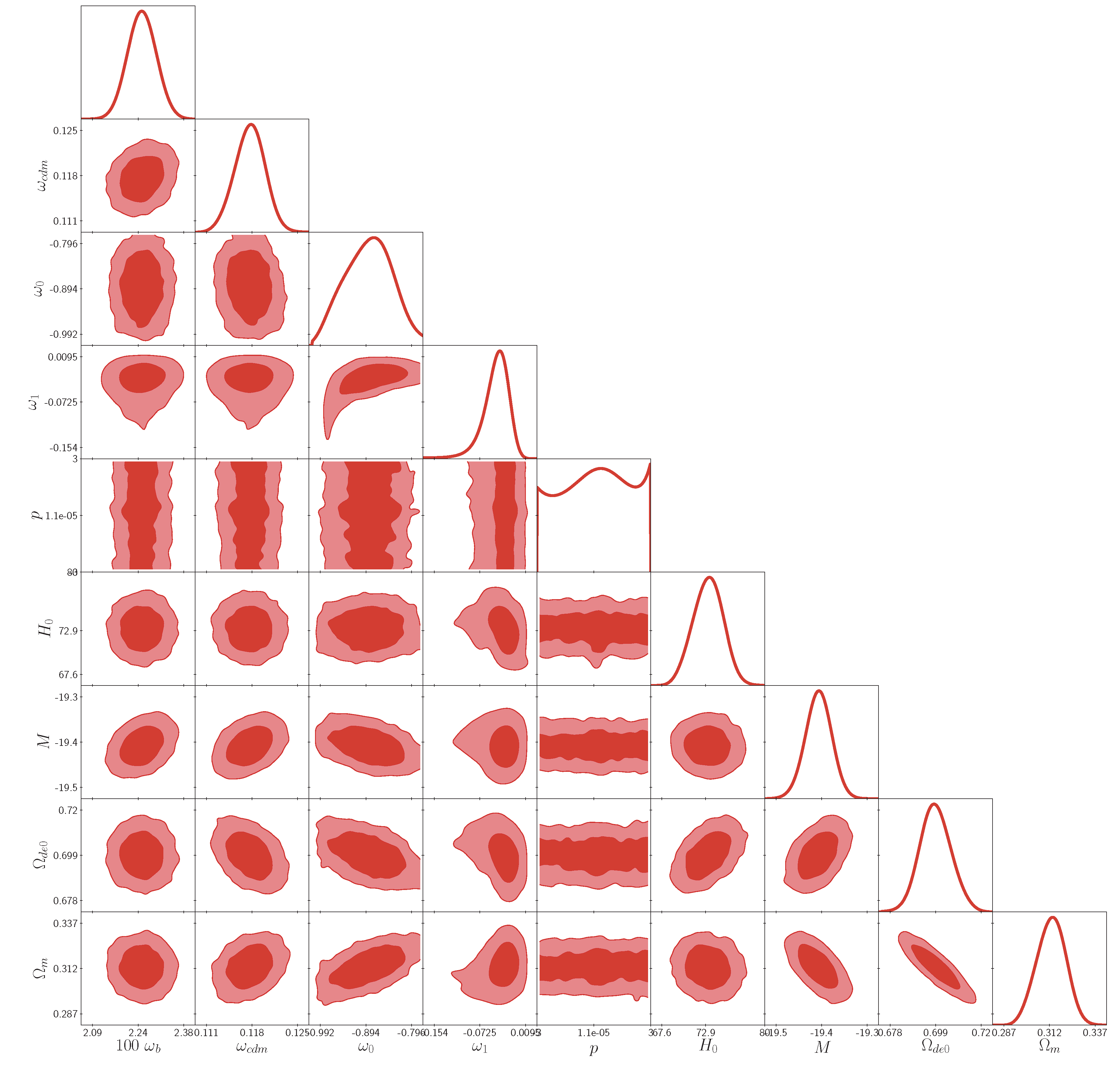
Figure 2.
The outlying panels show the 1D posterior distributions and 2D joint contours are drawn at and CL for the cosmological parameters for the Model I using data set ((Pantheon+) +BAO + HST) and PLANCK18 prior has been considered.
Figure 2.
The outlying panels show the 1D posterior distributions and 2D joint contours are drawn at and CL for the cosmological parameters for the Model I using data set ((Pantheon+) +BAO + HST) and PLANCK18 prior has been considered.
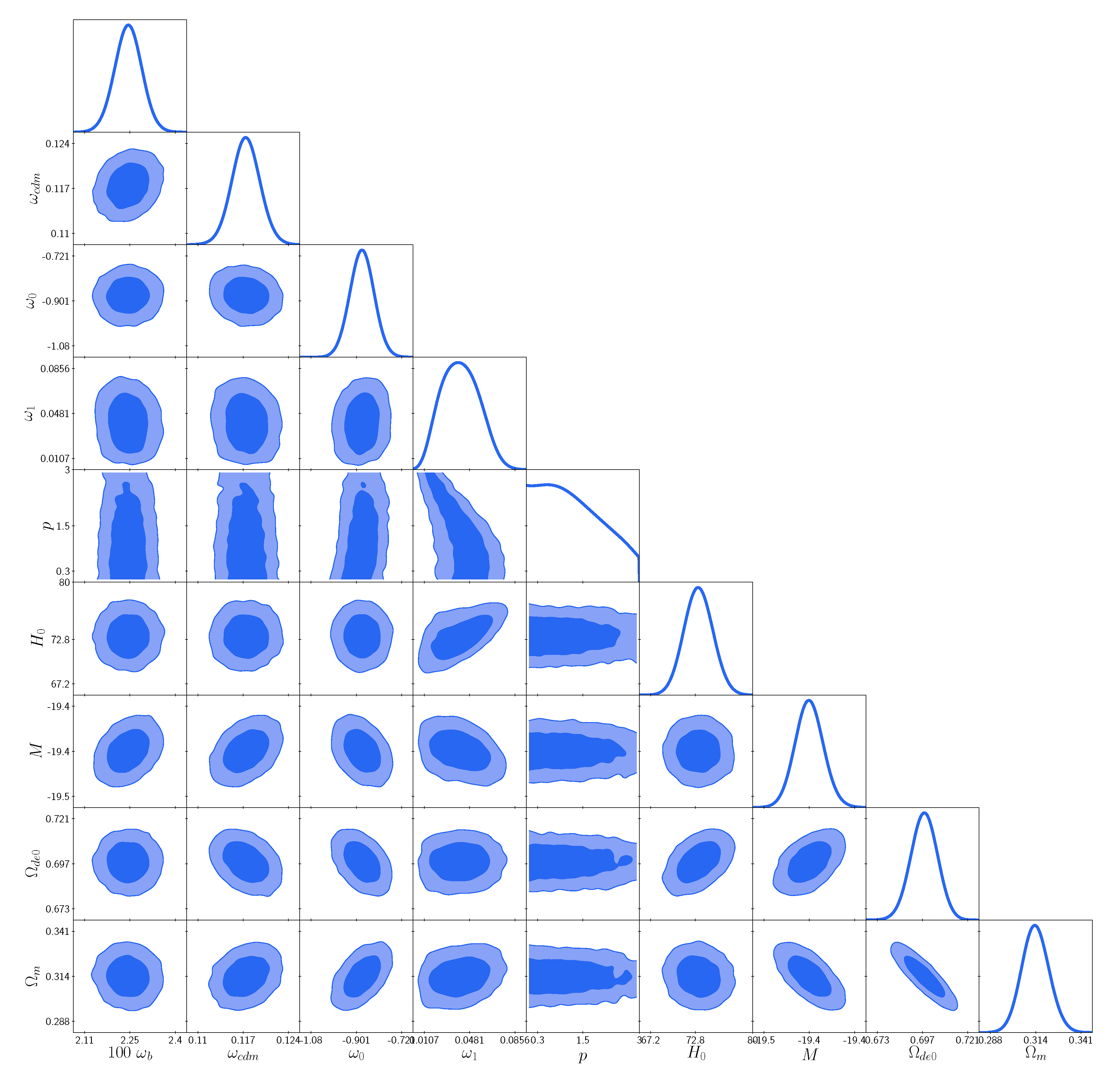
Figure 3.
Using the bestfit value inferred from the datasets (Pantheon+)+BAO+HST, the plots have been drawn for the different cosmological parameters. The solid red line and blue dashed line represent the Model I and Model II, respectively.
Figure 3.
Using the bestfit value inferred from the datasets (Pantheon+)+BAO+HST, the plots have been drawn for the different cosmological parameters. The solid red line and blue dashed line represent the Model I and Model II, respectively.
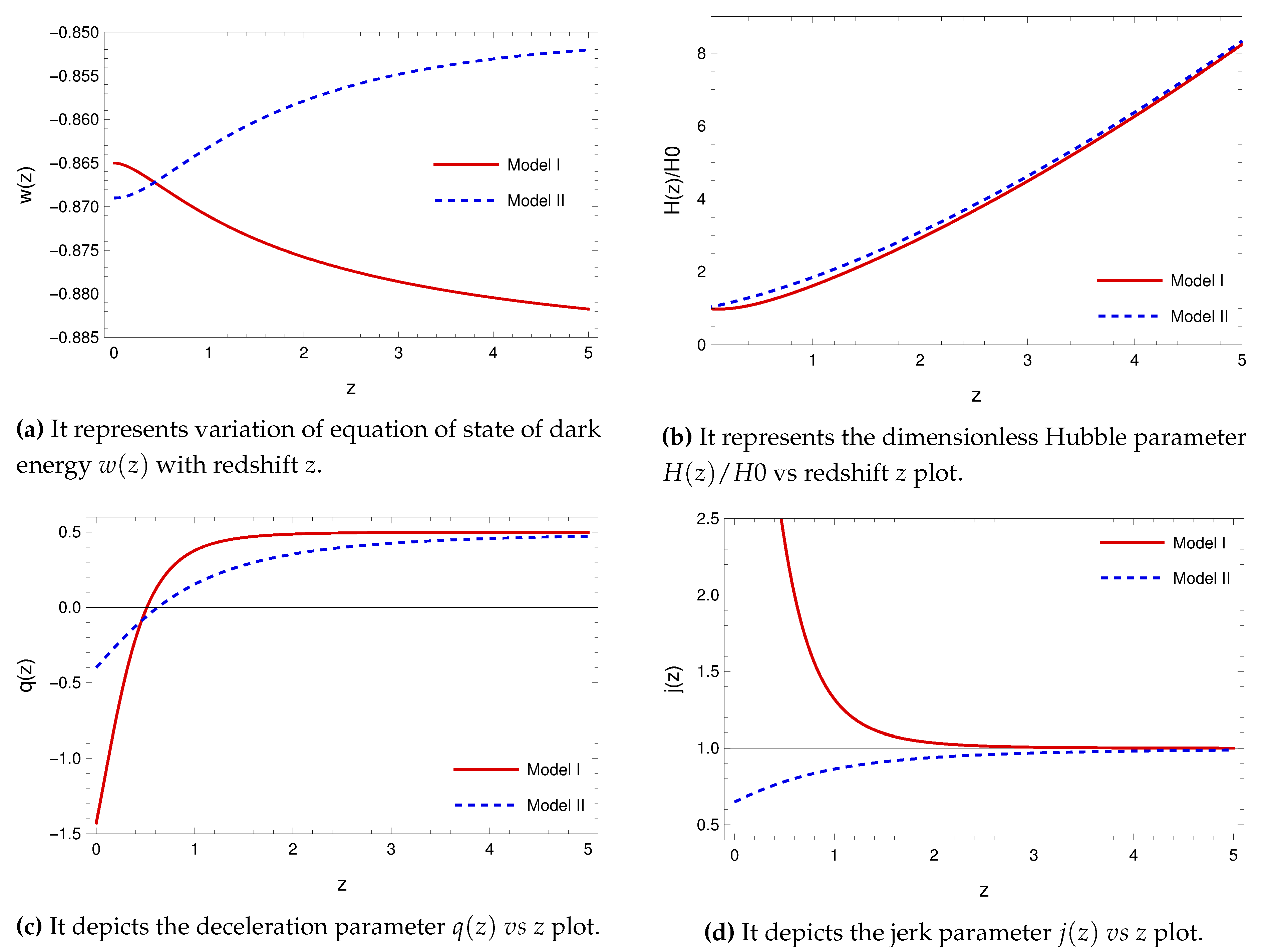

Table 1.
Best-fit values of model parameters for the different models using data sets ((Pantheon+) + BAO+HST).
Table 1.
Best-fit values of model parameters for the different models using data sets ((Pantheon+) + BAO+HST).
| Model I | Model II | |||
|---|---|---|---|---|
| Param | best-fit | mean | best-fit | mean |
| p | 1.975 | 2.283 | ||
| M | ||||
| 553.7 | 553.8 | |||
Table 2.
The values for the AIC and BIC for the different models
| (Pantheon+) +BAO+HST | ||||
|---|---|---|---|---|
| Model I | 567.79 | 605.89 | -296.282 | 0.997 |
| Model II | 567.887 | 605.98 | -297.279 | 0 |
Table 3.
| Notes | |
| Inconclusive | |
| 1.0 | Positive evidence |
| 2.5 | Moderate evidence |
| 5.0 | Strong evidence |
Disclaimer/Publisher’s Note: The statements, opinions and data contained in all publications are solely those of the individual author(s) and contributor(s) and not of MDPI and/or the editor(s). MDPI and/or the editor(s) disclaim responsibility for any injury to people or property resulting from any ideas, methods, instructions or products referred to in the content. |
© 2023 by the authors. Licensee MDPI, Basel, Switzerland. This article is an open access article distributed under the terms and conditions of the Creative Commons Attribution (CC BY) license (http://creativecommons.org/licenses/by/4.0/).
Copyright: This open access article is published under a Creative Commons CC BY 4.0 license, which permit the free download, distribution, and reuse, provided that the author and preprint are cited in any reuse.


