Submitted:
31 August 2023
Posted:
04 September 2023
You are already at the latest version
Abstract
Tracking temperature changes in certain geographic regions is a current task in modern research on Earth's climate changes. One of the global problems in solving this task is related to the large volume of measured data and the search for appropriate methods for effective determination of changes. The purpose of this research is to track climate temperature changes using a machine learning-based automated change detection method. The presented method includes training of a two-level structure of neural networks, with measured temperatures for a ten-year period of time for a certain geographical region. In the testing phase, the neural structure classifies measured temperatures for two three-year periods, before and after the ten-year time period, respectively, for the same geographic region. An algorithm was developed to visualize the studied regions by creating a map with their geographic coordinates. The classification results in the neural structure outputs are presented and analyzed as possible temperature changes. Suggestions for continuing and expanding the research in the future are discussed.
Keywords:
machine learning
; neural networks
; temperature changes
; geografical coordinates
1. Introduction
Today’s prevailing discussions and research in the field of climate change relate to the climate system today, to development of weather monitoring tools for accurate temperature measurement [1], organizing international forums about the human and ecological impacts of warming [2], etc. Data are presented and analyzed regarding the causes and consequences of global changes in Earth’s climate, including the latest climate data, a discussion of the earth’s carbon cycle, the warming hiatus of the first decade of this century, the 2017 hurricanes, advanced energy options [3]. According to an ongoing temperature analysis led by scientists at NASA’s Goddard Institute for Space Studies (GISS), the average global temperature on Earth has increased by at least 1.1° Celsius (1.9° Fahrenheit) since 1880. The majority of the warming has occurred since 1975, at a rate of roughly 0.15 to 0.20°C per decade, which is worrying about the possible consequences on a global scale [4]. Most current research in this area with the application of machine learning focuses on neural Earth system modeling by integrating artificial intelligence in Earth system science, but almost always affecting the Earth’s global temperature changes or changes in other climate parameters [5]. Researchers regularly analyze the obstacles in climate modeling, according to the current capabilities of modern technologies for processing large data sets and the extraction of features with the help of machine learning, as a subset of artificial intelligence [6].
Thus, the study of temperature changes in local geographic regions with the help of machine learning of neural networks (representing the “brain” of artificial intelligence) is relevant due to their adaptive abilities and the possibility of being trained to extract features, processing large datasets. The purpose of this research is to propose and investigate a method for tracking the climate temperature changes in a local geographic area, using a machine learning-based automated change detection method. The presented method includes training of a two-level structure of neural networks, given in Figure 1. At the first level, a preliminary clustering of measured temperature values at 30 points with three different values of Longitude and 10 values of Latitude geographic coordinates from the territory of France is performed, by means of training a neural network of Kohonen feature map type. This network is trained with measured temperatures for a ten-year period of time for these train points. In this way, a preliminary grouping of the regions into separate classes is obtained according to the degree of similarity in temperature changes over a 10-year period. Thus, the train data, grouped into classes is fed to the input of an MLP-type neural network, which represents the second level in the neural structure. An algorithm was developed, to create an interactive geographic map to find 17 cities (checkpoints/test points) geographical closest to the training points and to visualize on the map all train and test points. In the testing phase, the neural structure classifies measured temperatures for these 17 points, for two three-year periods, before and after the ten-year time period, respectively, for the same geographic region. The results indicate whether the temperature of nearby test points has changed in periods outside the ten-year period for train points.
2. Method description
The developed preprocessing software module aims to prepare the data for the experiment by: (1) determining the training points of the designed two-level neural network structure, (2) determining the test points for verifying the performance of the system (the nearby cities with monthly average temperature data), ( 3) for each test point, find the nearest training point. The software module uses two input-data files for its operation.
2.1. Interactive geographic map
The first file contains the training points. The training points file is in csv format with the following column names: longitude, latitude, January, February, March, April, May, June, July, August, September, October, November, December, Year. The columns with Month names contain the average temperature for the corresponding month, and the Year column contains the year in which the measurement was measured.
The second file is used to form the input data-set for the MLP neural network in the test phase of the two-level neural network structure. It contains the same temperature statistics for nearby selected cities. The file is in csv format with the following column names: dt, AverageTemperature, City, Country. The date of the average temperature measurement is recorded in the dt column in the format year-month-day. The measured average monthly temperature is recorded in the AverageTemperature column. The name of the city is recorded in the City column, and the name of the country - in the Country column.
The output of the described preprocessing stage is a data file for the selected cities, which includes: the name of the city, its geographic coordinates, the geographic coordinates of the nearest training point, the length of the line to it, and the average temperatures by month and year. An HTML file with an interactive geographic map is also generated. Training points are labeled in blue and control points in red. The lines connecting each city to its nearest training point are also shown on the interactive geographical map.
The software module is developed in Python using the Geopandas [7] and Folium library [8]. The coordinates of cities are determined based on their full names – city name, comma, country name. This is necessary to avoid possible duplication of city names in other countries. The coordinates are retrieved using the Geopy (a Python client for several popular geocoding web services) [9] and the Nominatim tool [10]. This approach eases the preliminary data preparation for system operation and enables users to use this system for arbitrary cities without having to locate their geographic coordinates, avoiding user errors.
Of interest is finding the closest test point to each “training” point. A function has been created to solve this task. The function takes as arguments two objects of type GeoDataFrame, describing the тест points and the training points, with the coordinates specified as objects of type Point and the names of the columns containing those coordinates. The function performs the following steps: (1) retrieves the coordinates of the training points and stores them in a list, (2) for each control point, finds the closest point from the created list and generates an object of type GeoDataFrame with 2 columns: test point, most -nearby training point. The function returns a list of the data from the second column of the generated GeoDataFrame object. This list is assigned as a new column to the object containing the test points.
HeatMap of the folium plugin and the CircleMarker and PolyLine methods were used to create the interactive geographic map.
Data on average monthly temperatures from the territory of France, downloaded from kaggle.com [11], were used to form the training point file. It contains information about the 30 chosen training points and the average monthly temperatures for each point for the years between 2000 and 2010. The first, second, and third 10 points have longitudes of -0.75 respectively; 2.25 and 5.25. For each value of longitude, 10 points with a latitude of 49.25; 48.75; 48.25; 47.75; 47.25; 47.75; 47.25; 45.75; 44.75; 44.25 are determined. Data for the 17 nearby cities with average monthly temperatures from 2011 to 2013 and from 1997 to 1999 were used to form the test points. Data are taken from the file “GlobalLandTemperaturesByCity.csv” downloaded from kaggle.com - Climate Change: Earth Surface Temperature Data [12]. It contains data on average monthly temperatures for major cities on Earth by month from 1743 to 2015. The resulting interactive map is represented in Figure 2.
2.1. Training the neural network structure
The first step of the proposed method consists in training a self-organizing feature map-type (SOM) Kohonen neural network. It was trained with the described 30 chosen training points, the average monthly temperatures for each point for years between 2000 and 2010. The goal of this training is to achieve a priori grouping of the points into a certain class/cluster of input data, according to similarity in the change of average monthly temperatures for the years 2000 to 2010. The input data for the specified time period for three of the 30 training points respectively with Longitude -0.75; 2.25 and 5.25 and Latitude 47.25 are presented in Figure 3
The trained SOM neural network has a structure of 12 input neurons, 64 neurons, in the feature map and initial learning rate of 0.06. The structure showed the best results in the clustering of the submitted total 330 input combinations [11 years (2000-2010) x 30 points]. combinations into a common file with three main classes. The obtained results in the SOM neural network feature map show achieved three distinct clusters, which leads to the subsequent clustering of the data from these 330 input training. The newly obtained file serves as input training data fed to the MLP neural network of the next level in the general neural structure of Figure 1. The MLP neural network has a 12-9-3 three-layered structure (12 input neurons corresponding to the 12 temperature values for each of the 12 months; 9 in the hidden layer and three neurons in the output layer corresponding to the three classes defined by the SOM network). In the next test phase, the defined temperature data from the pre-processing stage are fed to the input of the trained MLP neural network for classification. These are the data for the nearest cities (the 17 points), grouped in two files with different test data for time periods from 1997 to 1999 and from 2011 to 2013, respectively. SOM was trained with 4367 iterations to reduce the learning rate to 0. The MLP was trained with 56273 iterations until reaching 1% of MSE (mean square error) in the output layer, applying the classic Backpropagation training algorithm. Figure 4 shows the аpplied SOM and MLP neural network structures.
3. Results
The results of the clustering obtained in the SOM feature map for the 300 input temperature combinations (11 years (2000-2010) x 30 points) are shown in Figure 5. The three main temperature groups stand out clearly, the data of which are shown relative to the specific 30 training points indicated by their geographical coordinates. The newly obtained file serves as input training data fed to the MLP neural network of the next level. As next follows the training of the MLP neural network with the newly obtained and defined in the previous paragraph file. In the next test phase, the defined temperature data from the pre-processing stage are fed to the input of the trained MLP neural network for classification. These are the data for the nearest cities (the 17 points), grouped in two files with different test data for time periods from 1997 to 1999 and from 2011 to 2013, respectively. The results of the classification in the test phase of the temperature data for the 17 closest geographically located points, in the three classes defined by SOM, are shown in Figure 6. The total number of parametric vectors with tested temperature data for the period 1997-1999 is 51. For class 1, the temperature data for 6 input parametric vectors were tested (2 points from Figure 2 with data for 1997, 1998, 1999); for class2 - 18 input parametric vectors (6 points from Figure 2 with data for 1997, 1998, 1999) and for class 3 - 27 input parametric vectors (9 points from Figure 2 with data for 1997, 1998, 1999).
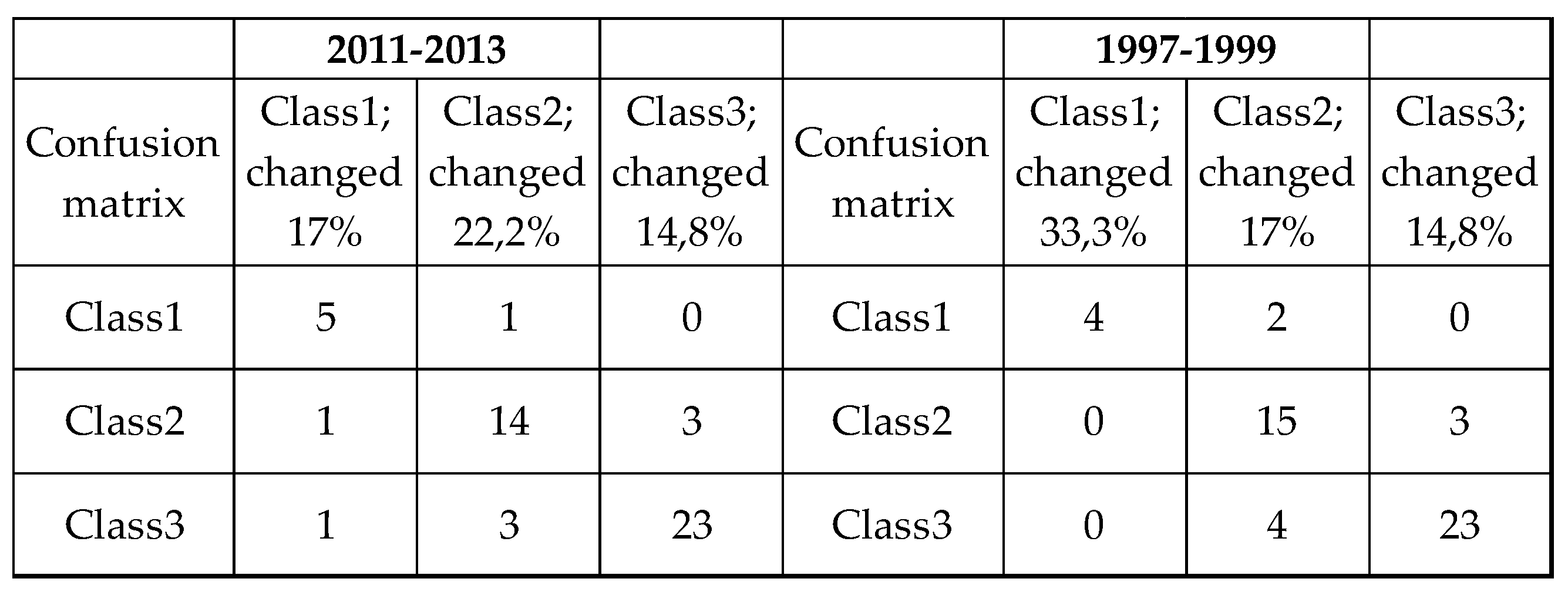
The same experiment for the same number of test points was also done for the temperature data of 2011, 2012 and 2013. The classification results of the MLP neural network, in addition to Figure 6, are also shown in Table 1 in the form of a confusion matrix.
The percentages of the classified temperature parametric vectors to classes, different according to the trained vectors, to adjacent geographical regions are indicated in Table 1 with “changed”.
4. Discussion
From the obtained Confusion matrix it is evident, that for class 1, only for one of the years 2011-2013 and only for two of the years 1997-1999, a classification of the temperature annual parametric vector to class 2 was obtained, i.e. to an adjacent territorially classified geographical area. This constitutes a 17% and 33.3% temperature zone shift, respectively.
The test data for class 2 show a preferential shift of 4 out of a total of 18 temperature annual parametric vectors preferentially to the geographical area of class3 for the annual range 2011-2013 and shift of 3 temperature annual parametric vectors preferentially to the geographical area of class 3 for the annual range 1997-1999. And for class 3 we can conclude that there is a shift of 14.8% preferentially towards the geographical area of class 2 for both annual ranges.
5. Conclusions
The presented research shows how, by combining known neural network models into a common structure, an automated analysis of trends in temperature shifts during selected annual periods of time for geographically adjacent local regions can be made. An advantage of the method is the absence of the need for complex calculations, because they are replaced only by one-time training of a large volume of data in multiple training iterations of neural networks. The length of training is not a limiting condition, when increasing the input data, since training is a one-time process. Pre-clustering the input data helps train the MLP neural network more accurately, which would aid its performance when dealing with larger datasets. In this direction, the intention of the authors is to continue the research for other geographical regions, with larger arrays of temperature data, in order to generalize the method.
References
- Available online: https://www.nist.gov/how-do-you-measure-it/how-do-you-measure-air-temperature-accurately (accessed on 21 July 2023).
- Available online: https://www.ghf-ge.org/human-impact-report.pdf (accessed on 19 July 2023).
- Kerry, E., Book, What We Know about Climate Change, Updated Edition, ISBN 9780262535915, Published: October 9, 2018, Publisher: The MIT Press. 9 October.
- Available online: https://data.giss.nasa.gov/gistemp/updates_v4/ (accessed on 19 July 2023).
- Irrgang, C. , Boers, N., Sonnewald, M. et al. Towards neural Earth system modelling by integrating artificial intelligence in Earth system science. Nat Mach Intell 3, pp. 667–674, 2021. [CrossRef]
- Available online: https://www.weforum.org/agenda/2021/08/how-is-machine-learning-helping-us-to-create-more-sophisticated-climate-change-models/ (accessed on 15 July 2023).
- 1x. GeoPandas documentation. Available online: https://geopandas.org/en/stable/docs.html (accessed on 30.08.2023).
- 2x. Folium library. Available online: https://python-visualization.github.io/folium/ (accessed on 30.08.2023).
- 3x. GeoPy’s documentation. Available online: https://geopy.readthedocs.io/en/stable/ (accessed on 30.08.2023).
- 4x. Nominatim Manual. Available online: https://nominatim.org/release-docs/develop/ (accessed on 30.08.2023).
- 5x. Available online: https://www.kaggle.com/datasets/shishu1421/global-temperature?select=air_temp (accessed on 15 June 2023).
- 6x. Climate Change: Earth Surface Temperature Data. Available online: https://www.kaggle.com/datasets/berkeleyearth/climate-change-earth-surface-temperature-data (accessed on 30 August 2023).
Figure 1.
Two-level neural network classification structure.
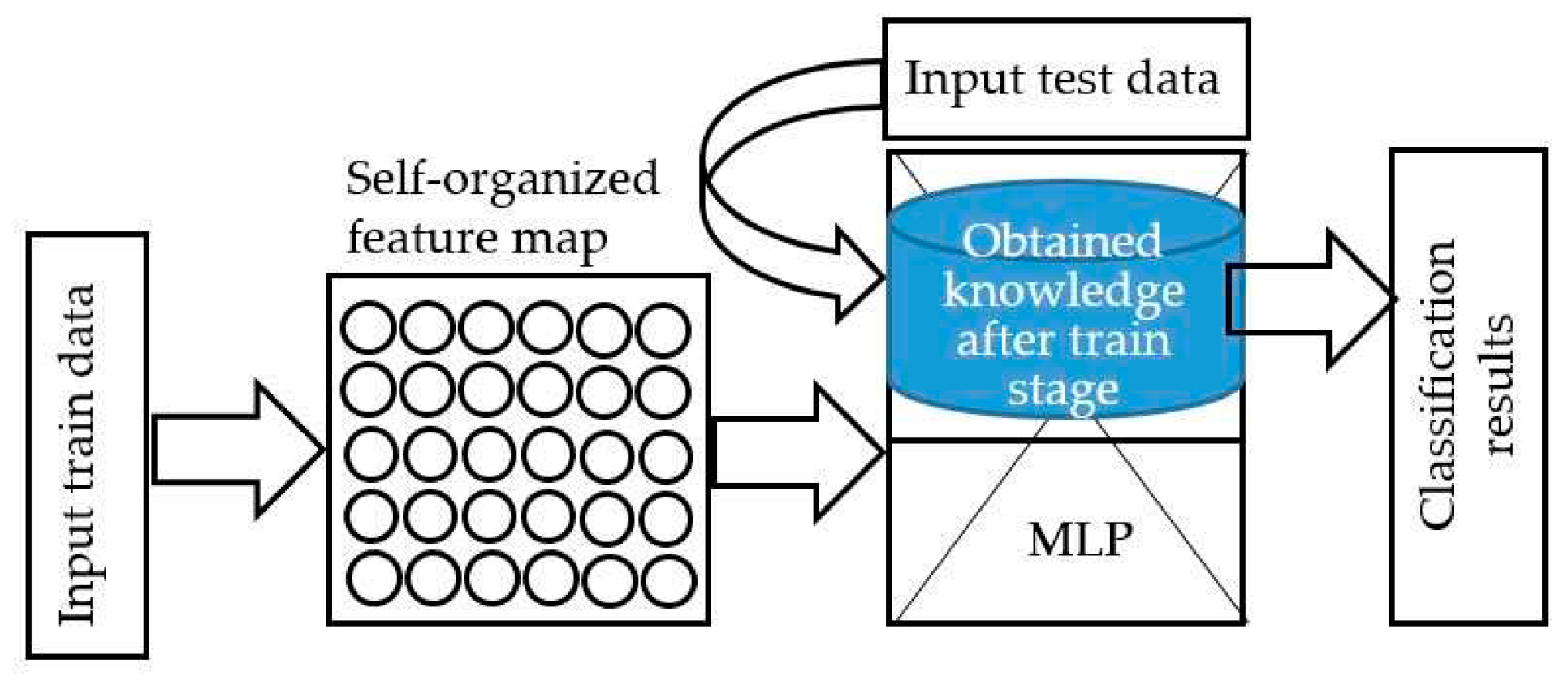
Figure 2.
Obtained interactive map with training and test point.
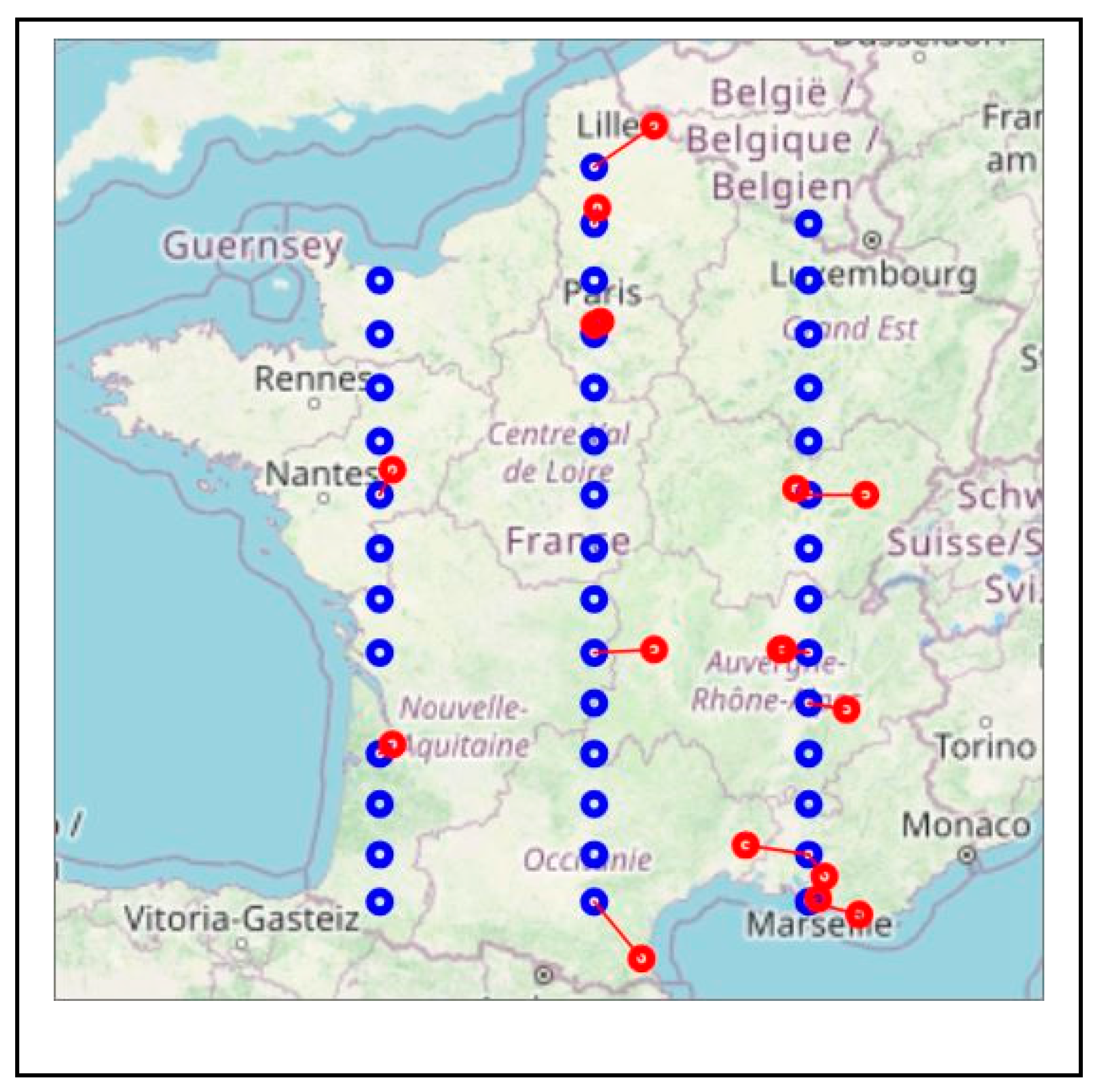
Figure 3.
Training data for 3 of 30 points as input set for SOM network
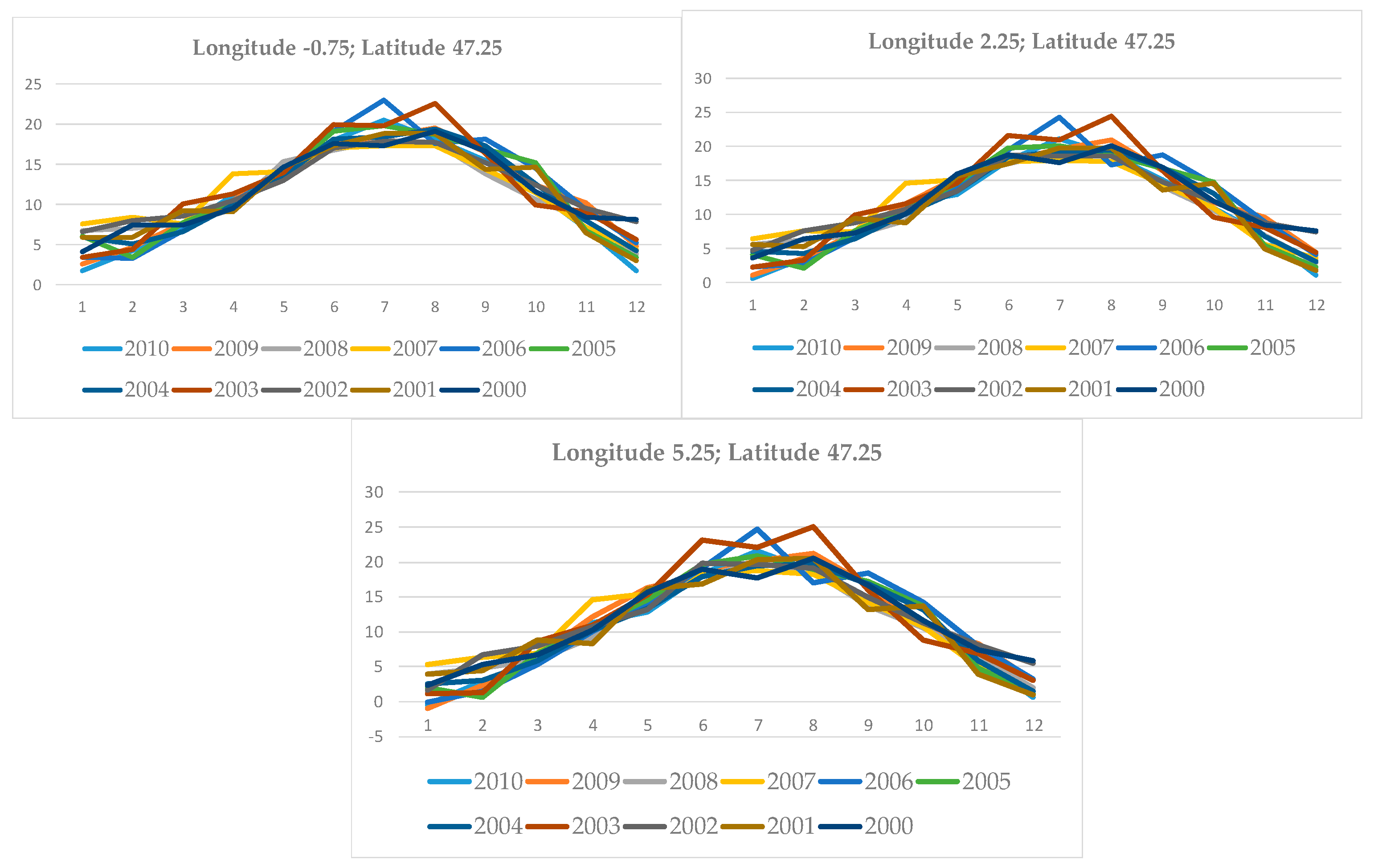
Figure 4.
The applied SOM and MLP neural network structures
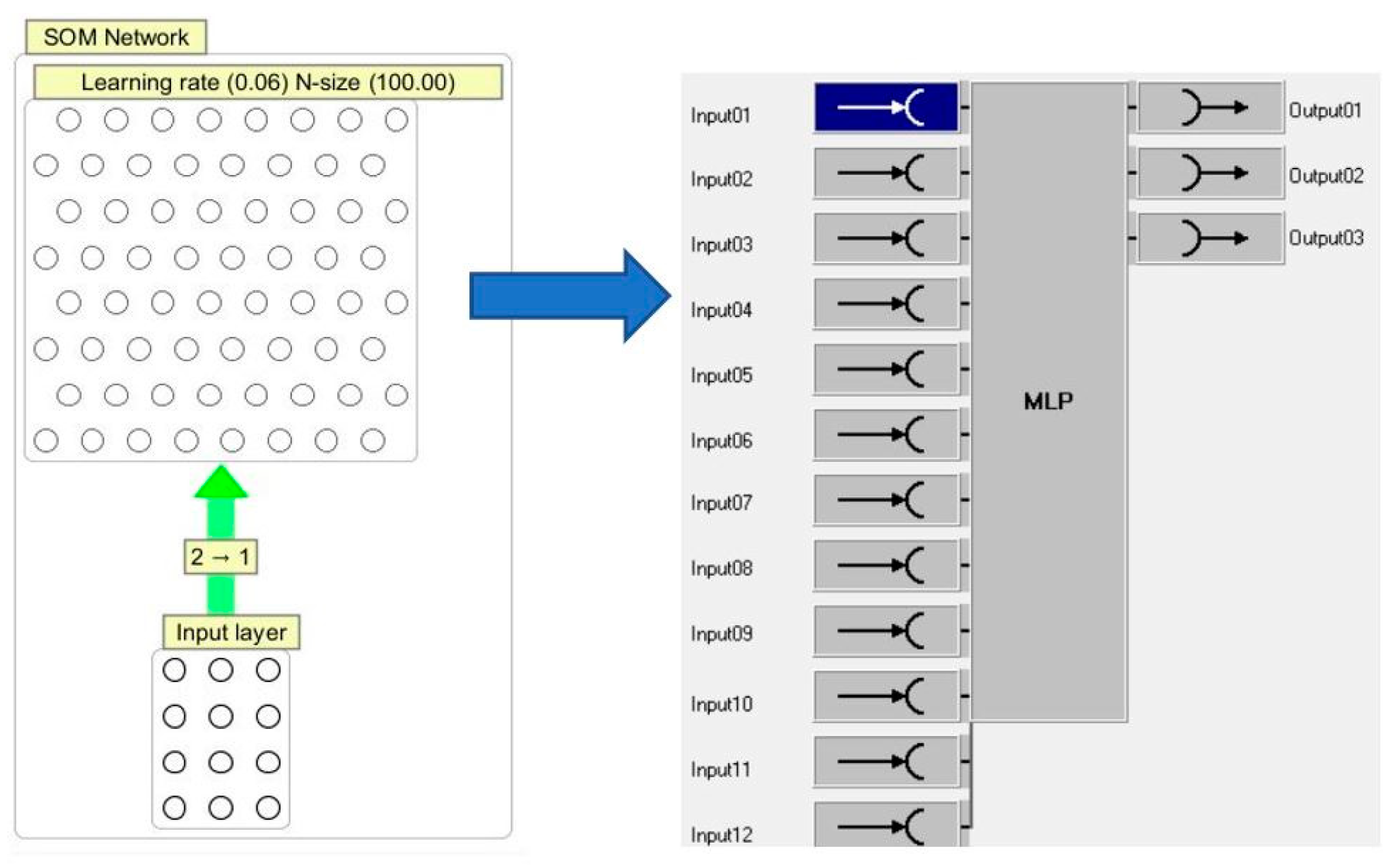
Figure 5.
The obtained clusters after training the SOM network.
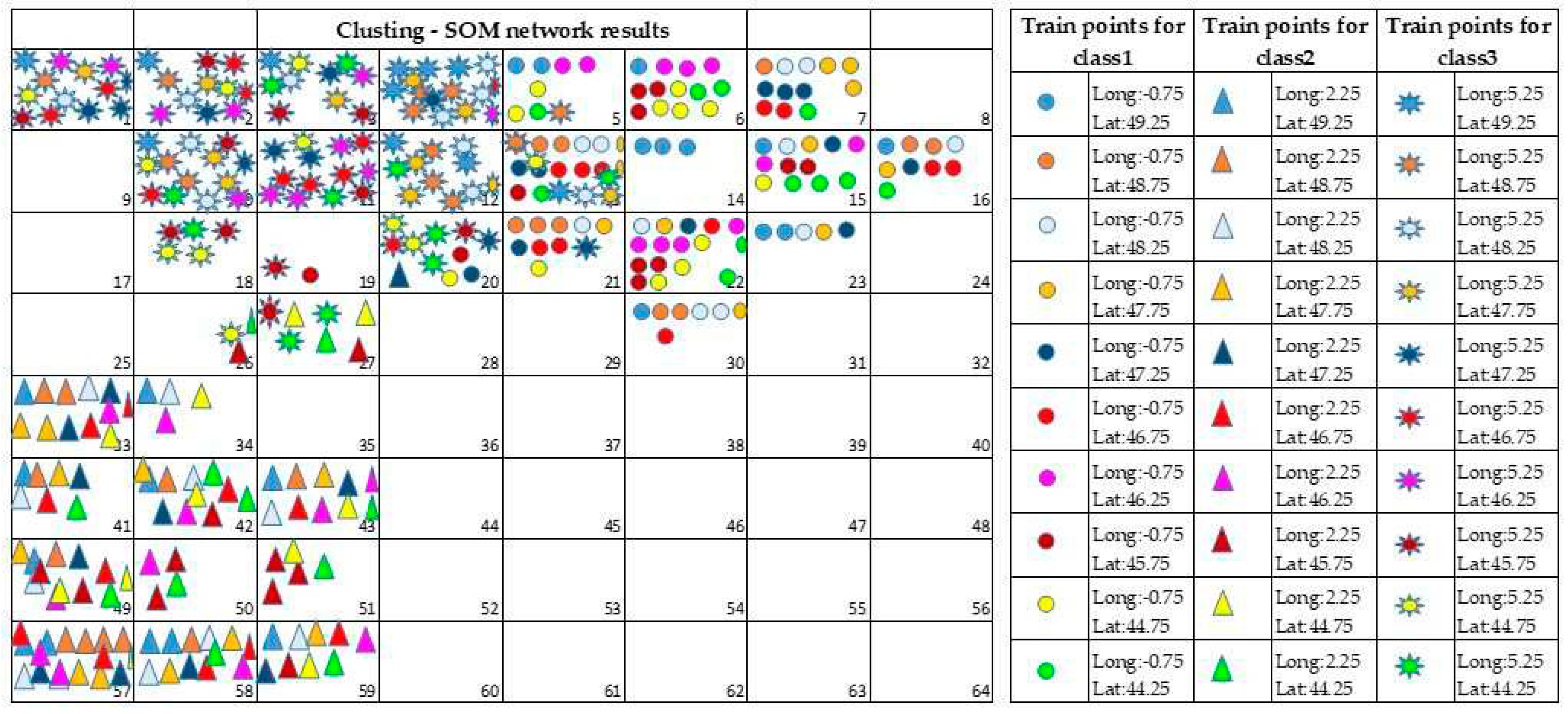
Figure 6.
The obtained test results for 51 test temperature parametric vectors for Years 1997 to 1999.
Figure 6.
The obtained test results for 51 test temperature parametric vectors for Years 1997 to 1999.
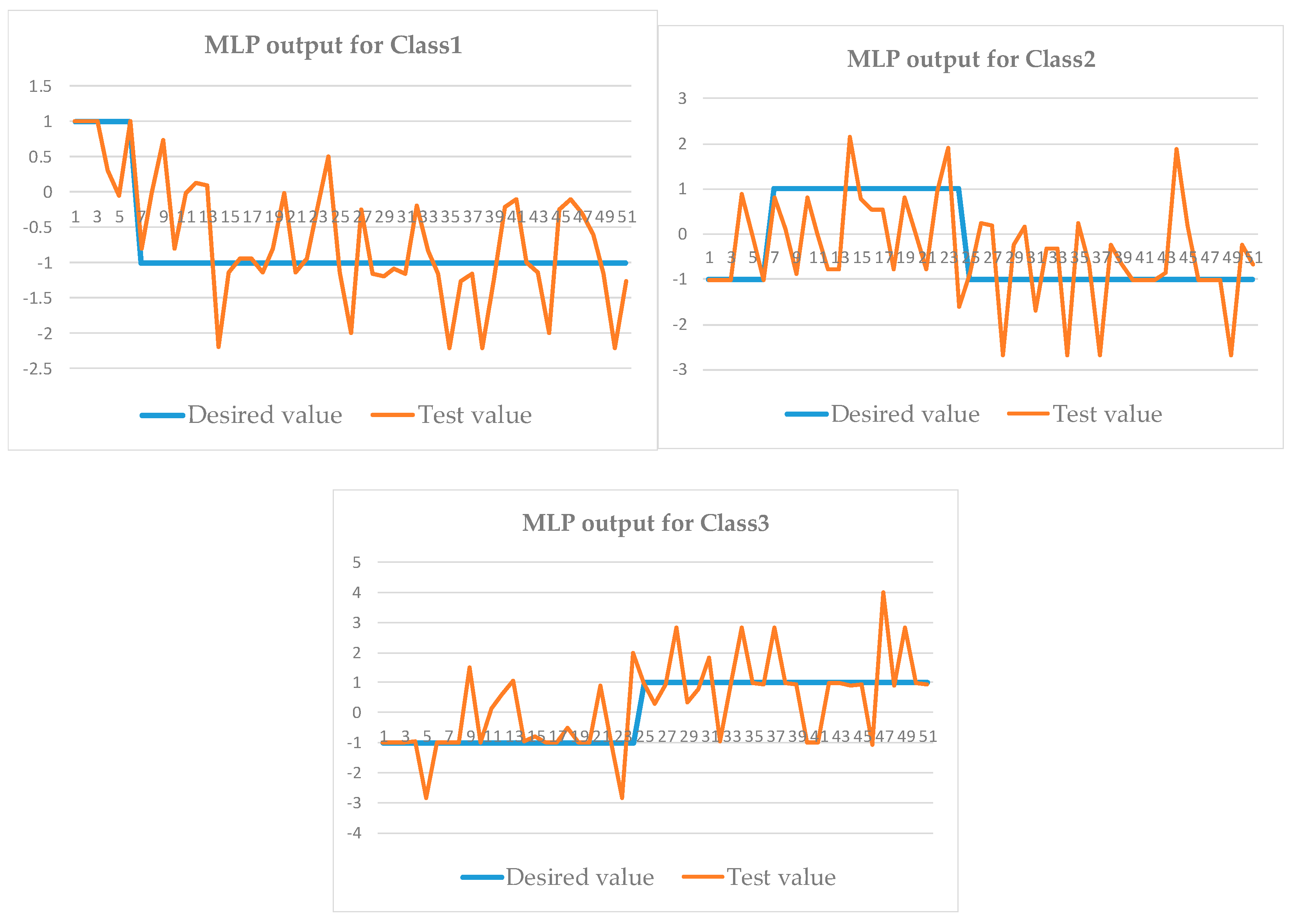

Table 1.
Confusion matrix for evaluation of classified 51 test points.
Disclaimer/Publisher’s Note: The statements, opinions and data contained in all publications are solely those of the individual author(s) and contributor(s) and not of MDPI and/or the editor(s). MDPI and/or the editor(s) disclaim responsibility for any injury to people or property resulting from any ideas, methods, instructions or products referred to in the content. |
© 2023 by the authors. Licensee MDPI, Basel, Switzerland. This article is an open access article distributed under the terms and conditions of the Creative Commons Attribution (CC BY) license (http://creativecommons.org/licenses/by/4.0/).
Copyright: This open access article is published under a Creative Commons CC BY 4.0 license, which permit the free download, distribution, and reuse, provided that the author and preprint are cited in any reuse.


