Submitted:
15 September 2023
Posted:
18 September 2023
You are already at the latest version
Abstract
We have found an infinite dimensional manifold of exact solutions of the Navier-Stokes loop equation for the Wilson loop in decaying Turbulence in arbitrary dimension $d >2$. This solution family is equivalent to a fractal curve in complex space $\mathbb C^d$ with random steps parametrized by $N$ Ising variables $\sigma_i=\pm 1$, in addition to a rational number $\frac{p}{q}$ and an integer winding number $r$, related by $\sum \sigma_i = q r$. This equivalence provides a \textbf{dual} theory describing a strong turbulent phase of the Navier-Stokes flow in $\mathbb R_d$ space as a random geometry in a different space, like ADS/CFT correspondence in gauge theory. From a mathematical point of view, this theory implements a stochastic solution of the unforced Navier-Stokes equations. For a theoretical physicist, this is a \textbf{quantum} statistical system with integer-valued parameters, satisfying some number theory constraints. Its long-range interaction leads to critical phenomena when its size $N \rightarrow \infty$ or its chemical potential $\mu \rightarrow 0$. The system with fixed $N$ has different asymptotics at odd and even $N\rightarrow \infty$, but the limit $\mu \rightarrow 0$ is well defined. The energy dissipation rate is analytically calculated as a function of $\mu$ using methods of number theory. It grows as $\nu/\mu^2$ in the continuum limit $\mu \rightarrow 0$, leading to anomalous dissipation at $\mu \propto \sqrt{\nu} \to 0$. The same method is used to compute all the local vorticity distribution, which has no continuum limit but is renormalizable in the sense that infinities can be absorbed into the redefinition of the parameters. The small perturbation of the fixed manifold satisfies the linear equation we solved in a general form. This perturbation decays as $t^{-\lambda}$, where the anomalous dimensions $\lambda$ satisfy the spectral equation \eqref{spectralEq}. The spectrum becomes a continuum in the statistical limit $N \to \infty$, presumably leading to multifractal phenomena.
Keywords:
Turbulence
; Fractal
; Anomalous dissipation
; Fixed point
; Velocity circulation
; Loop Equations
; Euler Phi
; Prime numbers
0. Introduction
In 1993, we derived [1,2] a functional equation for the so-called loop average [3,4] or Wilson loop in turbulence. The path to an exact solution by a dimensional reduction in this equation was proposed in the ’93 paper [2] but has just been explored.
At the time, we could not compare a theory with anything but crude measurements in physical and numerical experiments at modest Reynolds numbers. All these experiments agreed with the K41 scaling, so the exotic equation based on unjustified methods of quantum field theory was premature.
The specific prediction of the Loop equation, namely the Area law [2], could not be verified in DNS at the time with existing computer power.
The situation has changed over the last decades. No alternative microscopic theory based on the Navier-Stokes equation emerged, but our understanding of the strong turbulence phenomena grew significantly.
On the other hand, the loop equations technology in the gauge theory also advanced over the last decades. The correspondence between the loop space functionals and the original vector fields was better understood, and various solutions to the gauge loop equations were found.
In particular, the momentum loop equation was developed, similar to our momentum loop used below [5,6,7]. Recently, some numerical methods were found to solve loop equations beyond perturbation theory [8,9].
The loop dynamics was extended to quantum gravity, where it was used to study nonperturbative phenomena [10,11].
All these old and new developments made loop equations a major nonperturbative approach to gauge field theory.
So, it is time to revive the hibernating theory of the loop equations in turbulence, where these equations are much simpler.
The latest DNS [12,13,14,15] with Reynolds numbers of tens of thousands revealed and quantified violations of the K41 scaling laws. These numerical experiments are in agreement with so-called multifractal scaling laws [16].
Theoretically, we studied the loop equation in the confinement region (large circulation over large loop C), and we have justified the Area law, suggested back in ’93 on heuristic arguments [2].
This law says that the tails of velocity circulation PDF in the confinement region are functions of the minimal area inside this loop.
It was verified in DNS four years ago [12], which triggered the further development of the geometric theory of turbulence[14,15,17].
In particular, the Area law was justified for flat and quadratic minimal surfaces, and an exact scaling law in confinement region was derived [17]. The area law was verified with better precision in [13].
These exciting developments explain and quantitatively describe many interesting phenomena but do not provide a complete microscopic theory covering the full inertial range of turbulence without simplifying assumptions of the sparsity of vortex structures.
In the present work, we develop the theory free of these assumptions and approximations by solving the loop equations for decaying turbulence.
Our solution is irregular (local vorticity and local enstrophy limit do not exist), thus resembling the Tao conjecture [18]. There is an important difference though.
We are not studying singular solutions of the Navier-Stokes equations; rather we are solving the Hopf equations for a generating functional for the distribution of velocity circulation. We are looking for a statistical ensemble of Navier-Stokes solutions, and we arrive at the probability distribution. This distribution is singular in the sense that expectation values of powers of local vorticity diverge in a local limit.
At the same time, the correlation functions have singularities at coinciding points.
The correlation functions of vorticity at separated points are studied in the forthcoming paper [19] by numerical simulation of our theory. These correlations have power singularities at coinciding points, showing new fractal dimensions.
1. Loop equation
1.1. Loop operators
We introduced the loop equation in the Lecture Series at Cargese and Chernogolovka Summer Schools [2].
Here is a summary for the new generation.
We write the Navier-Stokes equation as follows
The Wilson loop average for the turbulence
treated as a function of time and a functional of the periodic function (not necessarily a single closed loop), satisfies the following functional equation
We added a dimensionless factor in the exponential compared to some previous definitions as an extra parameter of the Wilson loop. Without loss of generality, we shall assume that . The negative corresponds to a complex conjugation of the Wilson loop.
In Abelian gauge theory, this parameter would be the continuous electric charge.
The statistical averaging corresponds to initial randomized data, to be specified later.
The area derivative is related to the variation of the functional when the little closed loop is added
In the review, [2,17], we present the explicit limiting procedure needed to define these functional derivatives in terms of finite variations of the loop while keeping it closed.
All the operators are expressed in terms of the spike operator
The area derivative operator can be regularized as
and velocity operator (with )
In addition to the loop equation, every valid loop functional must satisfy the Bianchi constraint [3,4]
In three dimensions, it follows from identity ; in general dimension , the dual vorticity is an antisymmetric tensor with components. The divergence of this tensor equals zero identically.
However, for the loop functional, this restriction is not an identity; it reflects that this functional is a function of a circulation of some vector field, averaged by some set of parameters.
This constraint was analyzed in [17] in the confinement region of large loops, where it was used to predict the Area law. The area derivative of the area of some smooth surface inside a large loop reduces to a local normal vector. The Bianchi constraint is equivalent to the Plateau equation for a minimal surface (mean external curvature equals zero).
In the Navier-Stokes equation, we did NOT add artificial random forces, choosing instead to randomize the initial data for the velocity field.
These ad hoc random forces would lead to the potential term [17] in the loop Hamiltonian , breaking certain symmetries needed for the dimensional reduction we study below.
With random initial data instead of time-dependent delta-correlated random forcing, we no longer describe the steady state (i.e., statistical equilibrium) but decaying turbulence, which is also an interesting process, manifesting the same critical phenomena.
The energy is pumped in at the initial moment and slowly dissipates over time, provided the viscosity is small enough, corresponding to the large Reynolds number we are studying.
1.2. Dimensional reduction
The crucial observation in [2] was that the right side of the Loop equation, without random forcing, dramatically simplifies in functional Fourier space. The dynamics of the loop field can be reproduced in an Ansatz
The difference with the original definition of is that our new vector function depends directly on rather then through the vector field in projected at .
This transformation is the dimensional reduction we mentioned above.
From the point of view of the quantum analogy, this Anzatz is a plane wave in the Loop space, solving the Schrödinger equation in the absence of forces (potential terms in the Hamiltonian, depending on our position C in the loop space).
The reduced dynamics must be equivalent to the Navier-Stokes dynamics of the original field. With the loop calculus developed above, we have all the necessary tools to ensure this equivalence.
Let us stress an important point: the function is independent of the loop C. As we shall see later, it is a random variable with a universal distribution in functional space.
This independence removes our objection (see the Introduction) to the Kelvinon theory [20] and any other Navier-Stokes stationary solutions with a singularity at fixed loop C in space.
The functional derivative, acting on the exponential in (11), could be replaced by the derivative as follows
The loop equation for as a function of and also a function of time, reads:
where the operators should be regarded as ordinary numbers, with the following definitions.
The spike derivative D in the above equation
The first observation about this equation is that the viscosity factor cancels after the substitution (14).
As we shall see, the viscosity enters initial data so that at any finite time t, the solution for P still depends on viscosity.
Another observation is that the spike derivative turns to the discontinuity in the limit
The relation of the operators in the QCD loop equation to the discontinuities of the momentum loop was noticed, justified, and investigated in [6,7].
The momentum loop could be piecewise constant with an arbitrary number of such discontinuities.
In the Navier-Stokes theory, this relation provides the key to the exact solution.
In the same way, we find the limit for vorticity
and velocity (skipping the common argument )
The Bianchi constraint is identically satisfied as it should
We arrive at a singular loop equation for
This equation is complex due to the irreversible dissipation effects in the Navier-Stokes equation.
The viscosity dropped from the right side of this equation; it can be absorbed in units of time. Viscosity also enters the initial data, as we shall see in the next section on the example of the random rotation.
However, the large-time asymptotic behavior of the solution would be universal, as it should be in the Turbulent flow.
We are looking for a degenerate fixed point [17], a fixed manifold with some internal degrees of freedom. The spontaneous stochastization corresponds to random values of these hidden internal parameters.
Starting with different initial data, the trajectory would approach this fixed manifold at some arbitrary point and then keep moving around it, covering it with some probability measure.
The Turbulence problem is to find this manifold and determine this probability measure.
1.3. Random global vorticity
Possible initial data for the reduced dynamics were suggested in the original papers [2,17]. The initial velocity field’s simplest meaningful distribution is the Gaussian one, with energy concentrated in the macroscopic motions. The corresponding loop field reads (we set for simplicity in this section)
where is the velocity correlation function
The potential part drops out in the closed loop integral.
The correlation function varies at the macroscopic scale, which means that one could expand it in the Taylor series
The first term is proportional to initial energy density,
and the second one is proportional to initial energy dissipation rate
where is the dimension of space.
The constant term in (24) as well as terms drop from the closed loop integral, so we are left with the cross-term , which reduces to a full square
This distribution is almost Gaussian: it reduces to Gaussian one by extra integration
The integration here involves all independent components of the antisymmetric tensor . Note that this is ordinary integration, not the functional one.
The physical meaning of this is the random uniform vorticity at the initial moment.
However, as we see it now, this initial data represents a spurious fixed point unrelated to the turbulence problem.
It was discussed in our review paper [17]. The uniform global rotation represents a fixed point of the Navier-Stokes equation for arbitrary uniform vorticity tensor.
Gaussian integration by keeps it as a fixed point of the Loop equation.
The right side of the Navier-Stokes equation vanishes at this special initial data so that the exact solution of the loop equation with this initial data equals its initial value (27).
Naturally, the time derivative of the momentum loop with the corresponding initial data will vanish as well.
It is instructive to look at the momentum trajectory for this fixed point.
The functional Fourier transform [2,17] leads to the following simple result for the initial values of .
In terms of Fourier harmonics, this initial data read
The constant part of is not defined, but it drops from equations by translational invariance.
Note that this initial data is not real, as . Positive and negative harmonics are real but unequal, leading to a complex Fourier transform. At fixed tensor the correlations are
This correlation function immediately leads to the uniform expectation value of the vorticity
The uniform constant vorticity kills the linear term of the Navier-Stokes equation in the original loop space, involving .
The nonlinear term vanishes in the coordinate loop space only after integration around the loop.
Here are the steps involved
The tensor area was defined in (6). It is an antisymmetric tensor; therefore its trace with a symmetric tensor vanishes.
This calculation demonstrates how an arbitrary uniform vorticity tensor satisfies the loop equation in coordinate loop space.
We expect the turbulent solution of the loop equation to be more general, with the local vorticity tensor at the loop becoming a random variable with a non-Gaussian distribution for every point on the loop.
1.4. Decay or fixed point
The absolute value of loop average stays below 1 at any time, which leaves two possible scenarios for its behavior at a large time.
The Decay scenario in the nonlinear ODE (21) corresponds to the decrease of .
Omitting the common argument , we get the following exact time-dependent solution (not just asymptotically, at ).
The Fixed Point would correspond to the vanishing right side of the momentum loop equation (21). Multiplying by and reducing the terms, we find a singular algebraic equation
The fixed point could mean self-sustained turbulence, which would be too good to be true, violating the second law of Thermodynamics. Indeed, it is easy to see that this fixed point cannot exist.
The fixed point equation (43) is a linear relation between two vectors with coefficients depending on various scalar products. The generic solution is simply
with the complex parameter to be determined from the equation (43).
This solution is degenerate: the fixed point equation is satisfied for arbitrary complex .
The discontinuity vector aligned with the principal value corresponds to vanishing vorticity in (16), leading to a trivial solution of the loop equation .
We are left with the decaying turbulence scenario (42) as the only remaining physical solution.
2. Fractal curve in complex space
2.1. Random walk
One may try the solution where the discontinuity vector is proportional to the principal value. However, in this case, such a solution does not exist.
There is, however, another solution where the vectors are not aligned. This solution requires the following relations
These relations are very interesting. The complex numbers reflect irreversibility, and lack of alignment leads to vorticity distributed along the loop.
Note that this relation is parametrically invariant (being local and independent of ).
Also, note that this complex vector is dimensionless, and the fixed point equation (47) is completely universal, up to a single dimensionless parameter . The viscosity dropped from this equation, and the dimension of vorticity is inverse time, which explains the factor .
These equations do not allow , so discontinuities must be present at every . In other words, our solution cannot be smooth: it is a fractal curve rather than a piecewise smooth curve with discontinuities at several points.
We approximate this fractal curve by a polygon, with piecewise constant and N gaps at equidistant angles . If the limit exists, we get the desired fractal curve with a discontinuity at every .
One can build such a solution as a limit of the Markov process by the following method. Start with a complex vector .
We compute the next values from the discontinuity equations (47).
2.2. Constraints imposed on a random step
A solution to these equations can be represented using a complex vector subject to two complex constraints
after which we can find the next value
We assume N steps, each with the angle shift .
This recurrent sequence is a Markov process because each step only depends on the current position . The closure requirement makes it a periodic Markov process, with the period N.
This requirement represents a nonlinear restriction on all the variables , which we discuss below.
With this discretization, the circulation can be expressed in terms of these steps
Note that the complex unit vector is not defined with the Euclidean metric in dimensions . Instead, we have a complex condition
which leads to two conditions between real and imaginary parts
In d dimensions, there are complex parameters of the unit vector; with an extra constraint in (50b), there are now free complex parameters at every step of our iteration, plus the discrete choice of the sign of the root in the solution of the quadratic equation (50b) for the projection .
2.3. Closure condition
At the last step, , we need to get a closed loop . This is one more constraint on the complex vectors
We use this complex vector constraint to fix some of the remaining parameters.
Due to the closure of the space loop , the global translation of the momentum loop leaves invariant the Wilson loop; this leads to certain gauge invariance (see below).
The circulation must correspond to a real number, though the Wilson loop is not real, as there is an asymmetry in the distribution of signs of circulation.
We discuss this issue in the following sections.
2.4. Mirror pairs of solutions
Return to the general study of the discrete loop equations (50).
There is a trivial solution to these equations at any even N
We reject this solution as unphysical: the corresponding vorticity equals zero, as all the vectors are aligned.
Our set of equations has certain mirror reflection symmetry
Thus, the complex solutions come in mirror pairs . The real solutions are only a particular case of the above trivial solution with real .
Each nontrivial solution represents a periodic random walk in complex vector space . The complex unit step depends on the current position , or, equivalently, on the initial position plus the sum of the preceding steps.
We are interested in the limit of infinitely many steps , corresponding to a closed fractal curve with a discontinuity at every point.
2.5. The degenerate fixed point and its statistical meaning
This solution’s degeneracy (fewer restrictions than the number of free parameters) is a welcome feature. One would expect this from a fixed point of the Hopf equation for the probability distribution.
This degeneracy leads to stochastization of the Navier-Stokes flow at large Reynolds numbers. The solution comes as a manifold, and the flow covers this manifold with some invariant measure.
In the best-known example, the microcanonical Gibbs distribution for Newton’s mechanics covers the energy surface with a uniform measure (ergodic hypothesis, widely accepted in Physics, though still unproven in Mathematics).
The parameters describing a point on this energy surface are not specified– in the case of an ideal Maxwell gas, these are arbitrary velocities of particles.
Likewise, the fixed manifold, corresponding to our fractal curve, is parametrized by sign variables, like an Ising model, plus an arbitrary global rotation matrix and a global parameter , as discussed in the next section.
This rich internal random structure of our fixed manifold, combined with its rotation and translation invariance in loop space C, makes it an acceptable candidate for extreme isotropic turbulence.
3. Exact analytic solution
3.1. Random walk on a circle
How could a complex curve describe real circulation? This magic trick is possible if the imaginary part of does not depend on .
Such an imaginary term will drop after integration over closed loop .
We have found a family of such solutions [21] of our recurrent equation (49) for arbitrary N
Here is a unit vector.
The angles must satisfy recurrent relation
This sequence with arbitrary signs solves recurrent equation (49) independently of .
The closure condition requires certain relations between these numbers.
The main condition is that must be a rational fraction of :
The case is eliminated. It corresponds to .
In that case, the periodic solution for will have correspond to the following set of
This array has positive values and negative values where
The symbol stands for a random permutation of the array, which preserves its sum
This sum must be a multiple of q for periodicity, which leads to another restriction
In other words, must have the same parity as N.
These properties lead to periodicity
At fixed denominator q, the winding number r can take the values
The sequence with all spins flipped: also solves the loop equation. This sequence is a reflected solution we mentioned, so we include it in the statistical samples with equal probability. It corresponds to the winding number’s reflection .
The number of states with given is a partition of positive and negative spins into N boxes. The probabilities are given by binomial distribution with
The next section discusses this ensemble of rational numbers and its statistics at .
Given the rational number , we can generate the sequence of angles , adding to a multiple.
The random walk step is a real unit vector in this solution
The direction of this vector is not random, though; in addition to the random sign and random unit vector in dimensions, its direction depends on the previous position on a circle.
So, this is a perfect example of a periodic Markov chain, with the periodicity condition analytically solved by quantizing the angular step to a rational number .
This solution corresponds to the real value of velocity circulation on each of these two solutions; however, the reflection changes this value.
Thus, the arithmetic average of two Wilson loops with two reflected solutions is reflection-symmetric, but it is still a complex number.
Our solution has a peculiar gauge invariance. The circulation and, therefore, all observables are invariant under the shift of all by a constant vector:
This gauge invariance follows from the closure of the loop C: any constant term in yields zero after integration , or summation .
Using this invariance, we can drop the last component of so that they become real vectors
The vorticity operator in this gauge will become a purely imaginary vector in the z direction:
As we shall see, this does not lead to complex numbers for the correlation functions of vorticity in physical space.
The correlation function of two vorticities, separated by a finite distance in an "inertial interval," is finite and real after integration over the global rotation matrix. Its limit at may be singular so that the anomalous dissipation may emerge.
This discrete set describes a particular solution of the loop equation for the Wilson loop in decaying turbulence.
Here is an important point to keep in mind. Unlike the Navier-Stokes equation, the loop equation is linear.
Therefore, any superposition of its solutions parametrized by also solves the loop equation. We need to find a particular superposition that has the correct physical properties.
In particular, this superposition must describe a continuum limit of our fractal curve when . In the next two sections, we study an ensemble of such solutions, the Euler ensemble. This ensemble corresponds to adding every solution with equal weight.
Naturally, the question arises: Why equal weight? Why not give the even N more weight or exclude prime numbers?
This is our ergodic hypothesis.
Equal weight is the most symmetric option from the mathematical point of view, plus the properties of such an ensemble can be studied by a number theory methods.
One argument favoring the equal weight hypothesis is that weight distribution may become irrelevant in the local limit.
This limit, as we shall see in the rest of the paper, is determined by the statistical weight of the configurations of the ensemble. Therefore, the singular behavior of the ensemble when the mean number of vertices in the fractal curve goes to infinity may be universal.
In other words, the continuum fractal curve corresponding to the limit of this solution may be a unique mathematical object independent of the method used to approximate it by a polygon.
In that case, there may be an alternative way to describe this fractal curve without taking a limit of a large polygon. This description would require more sophisticated mathematical methods than those we use in this paper.
The advantage of our polygonal approach to the fractal curve is that it is well-defined and is solvable (the ensemble averages are calculable) at every finite N and can be analytically extrapolated to the ensemble with .
In terms of modern QFT, the continuum limit of this statistical ensemble is dual to the statistical theory of the velocity field.
3.2. The Euler ensemble
The discrete set of fractions with denominator is well known in the number theory [24], starting with Euler.
However, our extra restriction ties the set of fractions to the set of N Ising variables. We will study the statistics of the corresponding ensemble, which we call the Euler ensemble, honoring my idol, Leonard Euler.
He never thought that his functions and his equation for ideal fluid would meet in theoretical physics, but a genius creates subconsciously.
We distinguish between big Euler ensembles and small Euler ensembles.
The big ensemble assigns equal weight for each element of the large set
The small ensemble results from averaging the big ensemble over the variables
The binomial coefficients count the number of states with among all states of the set of .
We divided the statistical weights (the number of allowed configurations) by the total number of spin configurations. This normalization makes the probability of finding the values in the big Euler ensemble with random .
Let us count all fractions with denominator and proper parity, same as N. All the integers between 2 and N are allowed for q, and each such number would enter with the weight .
At given the allowed numbers of p are all integers such that . The famous Euler’s totient [24] counts such numbers.
Thus, we can relate the big Euler ensemble average of some function to the small ensemble average as follows
The advantage of this representation is that we can first average by the variables, which is a rather simple arithmetic mean. After that, we have to average over the small Euler ensemble, which involves only three variables. Resulting triple sums are calculable numerically with Mathematica®and also can be studied in the local limit by the methods of number theory.
The odd and even ensembles have different asymptotic behavior with N.
Here are the allowed parity of for odd/even N
The ratios
were computed for (see Figure 1). These ratios are finite, up to some value of q, after which they quickly go to zero (faster than exponentially).
This fast decrease suppresses these terms in the sum over q, which otherwise diverges at the upper limit and grows as .
At large N the weight tends to the q- independent limit
which does not restrict the sum of Euler totients .
Therefore, for even N
For odd N, the leading term is missing, so we have to sum the terms with .
This term converges at where is not exponentially small. The asymptotic formulas for summators of the Euler totients do not apply here, so we can compute this sum numerically and extrapolate to .
It is a challenge to the number theory to produce exact asymptotic behavior, replacing my fitted "law."
Recently, the number theory answered this challenge [25]. The result of their computation confirms the factor but rejects the correction factor as an overfit due to insufficiently large N.
The actual pre-exponential coefficient is required for the full theory of the Euler ensemble. Still, it does not contribute to the leading term of the grand canonical ensemble we use in the rest of the paper.
The results of [25] correspond to without any factors of . This reminds us that mathematical laws must be derived theoretically rather than fitted to numerical data.
3.3. Grand canonical ensemble
The original Euler ensemble with fixed N can be regarded as a microcanonical ensemble of statistical mechanics.
The grand canonical ensemble is more appropriate if the number of states can fluctuate, as in our case, where probabilities drastically change when N is shifted by 1.
The weights for varying numbers N of degrees of freedom are multiplied by , then N is treated as the rest of the variables. The chemical potential will have to tend to zero in the thermodynamic limit, and the resulting singularity becomes a thermodynamic singularity corresponding to the critical phenomena.
Note that we changed the sign of compared to the historical definition: our so that the opposite sign would be inconvenient.
The partition function and the ensemble averages in the grand canonical ensemble are
With the grand canonical ensemble, the ambiguity of the local limit disappears. At the critical point , the even N dominate, with the following result
The extra factor of came from skipping all the odd values of N. The remaining sum over even N tends to be half the asymptotic expression’s integral for these even N.
In the rest of the paper, we shall use the grand canonical ensembles in the thermodynamic limit , where we find the critical phenomena.
With the grand canonical ensemble, the ergodic hypothesis becomes a weaker restriction: any smooth weight function in the distribution will cancel in expectation values in the limit . For example, the saddle point calculation yields
This phenomenon is "self-organized criticality," unlike conventional second-order phase transitions in statistical physics, which require tuning of thermodynamical potentials (temperature, pressure, chemical potential, etc.). The critical point does not require fine-tuning.
The self-organized criticality, or spontaneous stochastization of turbulence, is an expected property that was never proven theoretically but observed in numerical and real experiments.
In our theory, this spontaneous stochastization naturally emerges in the solution of the loop equations in the local limit.
4. Correlation functions
In this section and the rest of the paper, we only consider the three-dimensional space we inhabit. There are interesting mathematical problems related to decaying turbulence in higher dimensions, which we leave to future researchers. In less than three dimensions, our solutions do not exist.
4.1. General formulas
The simplest observable quantities we can extract from the loop functional are the vorticity correlation functions [17], corresponding to the loop C backtracking between two points in space , see Figure 3. The vorticity operators are inserted at these two points.
The correlation function reduces to the following average over the ensemble of our random curves in complex space.
The averaging in these formulas involves group integration with .
Let us explain the origin of summation over two positions of the points on the discreet loop .
There is a degree of freedom we did not specify until now, namely, the reparametrization of the momentum loop .
The loop equations (21) are invariant under the one-dimensional diffeomorphisms ( or reparametrizations)
Thus, the general solution involves an arbitrary monotonous function , and averaging over the fixed manifold of the solutions of the Navier-Stokes equations involves functional integration over all such functions.
This integration includes summation over the positions of the vorticity insertion points on a curve . In the continuum theory, this would be an ordered Lebesgue integration (diffeomorphisms preserve the ordering of points on a curve)
and in our case of piecewise constant curve with discontinuities , it becomes an ordered sum
The discontinuity stays finite in the continuum limit . The continuum limit can be taken only after integrating(summing) the internal degrees of freedom of the fixed manifold of the Loop equations.
The imaginary part of our solution (60) does not depend on the point on a circle. Therefore, it contributes a constant term into which cancels in the difference in the exponential, as it should.
Let us look at the correlation function (106).
First, we expand and simplify the dot product involved
4.2. Critical phenomena in statistical limit
Now we are prepared to average over spin variables .
This expression singles out the variables so we can sum over these two variables, leaving the rest of free, except for a constraint . This constraint can be implemented as a discrete Fourier integral:
We start with
Then we take the integral out of the sum:
This expression can be readily averaged over two variables , which reduces to the sum of four terms with . Keeping only the factors depending on
The next step would be averaging over the remaining variables . These variables are split into two sets: one is used in the , and the other is used in .
The variables have a certain distribution in the statistical limit when both . We also have in that limit.
We are now considering the unconstrained distribution over , as the constraint is implemented via the discrete Fourier integral.
Let us compute the mean and variance of
In the relevant critical region , the ratio of the variance of to the square of its mean tends to a finite limit
This function looks singular, but it is positive and finite in the allowed region ( see Figure 4).
Therefore, the CLT does not apply to the distribution of , and all the moments of this distribution must be computed to obtain the probability distribution as a Mellin transform.
This computation represents another challenge to the number theorists.
This complication is bad news for attempted direct computation but good news for our theory: we have critical phenomena with a non-Gaussian distribution in the statistical limit.
Still, in the next section, we derive an exact formula for the mean value of the enstrophy as a function of the chemical potential , relating it to the functions of the number theory.
4.3. Analytic solution for the enstrophy
Let us find analytic formulas for observables of this remarkable statistical distribution, which is isomorphic to the Ising model tied to the ensemble of fractions.
The one-dimensional Ising models are usually solvable, and this one is no exception.
The simplest quantity is the enstrophy related to our random variables in the previous section.
Setting in (106) (which is possible at finite N) we find the following relation
where the big Euler ensemble average denotes averaging over and the Ising variables subject to the global constraint .
The general theory in Section 3.2 expressed the big Euler ensemble average in terms of the small Euler ensemble average of the average over spins.
So, we start the computation of the enstrophy by averaging over spins , which is rather simple.
Let us use the explicit expression (114) for the dot product .
Now, using the one-dimensional Fourier integral for the global constraint on , we get the unconstrained average:
Averaging it over we find
Now, averaging over the remaining is straightforward.
We arrive at the integral
This integral is calculable (see [26]):
Summing over yields , leading to our final answer
We investigated this new function in [19], and represented it in terms of so-called multitotients [27]. For the reader’s convenience, we present the computations leading to this representation in Appendix A.
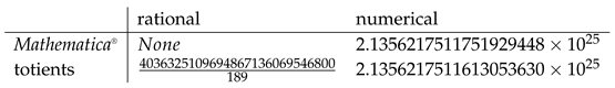
Here are prime factors of q. This remarkable identity can be directly verified using Mathematica®[28]. It takes over a minute of CPU to compute and simplify . The same result using the multitotient formula takes 140 microseconds.
Here is the table of for
This is an even integer for , and here is a simple proof.
Proof.
The second term in is an even integer, and the first term can be rewritten as
where is a multiplicity of the prime factor p. The remaining factors . The sequence of three integers has a factor divisible by three, and it cannot be p as it is a prime number, with the only exception being . Starting with there is always a factor of 3 either in or in or in any other prime factors analyzed above. The divisibility by 2 is similar: both factors for any prime are even, and any power with is divisible by 4. Therefore is divisible by 12, so that is divisible by 4. Thus is an even integer for . □
The plot of the first 100000 values of looks as follows (see Figure 5).
The appearance of prime numbers in the fluid dynamics problem is exciting; it reveals hidden relations between these different branches of modern mathematics. It reminds me of similar unexpected relations between matrix models, orthogonal polynomials, and 2D quantum gravity.
This formula is our exact solution for enstrophy, expressing it as a calculable average over the small Euler ensemble. In the next section, we compute it in the local limit .
4.4. The local limit of the energy dissipation
In the limit , the term with zero winding dominates the sum , which is only possible for even N. Its asymptotic limit is
The remaining terms, with can be replaced by an integral of the asymptotic expansion of the exact expression
The leading term cancels after integration, so the contribution dominates the sum.
The next term of expansion in cancels as well
We do not need this term , as the dominant term grows as . As seen in the Section 3.2, the remaining terms decrease faster than exponential with q, making it a nontrivial exercise in number theory to find an analytic formula for the partition function and the enstrophy in the odd Euler ensemble.
Let us concentrate on even N, as this term dominates the grand canonical ensemble we study.
The extra factor of came from skipping all the odd values of N. The remaining sum over even N tends to be half the asymptotic expression’s integral for these even N.
The asymptotic behavior of multitotient summators has been known for a century [27]
where is the Riemann’s zeta function.
We obtain the following local limit of the energy decay in the grand canonical Euler ensemble
This energy dissipation stays finite in a turbulent limit provided
Let us now estimate the odd N contribution to the enstrophy. Here, the sum of the spin average is dominated by , where we cannot use the asymptotic formula of the number theory for totients.
Thus, we used numerical results of direct computations of the small Euler ensemble contribution from odd N to the enstrophy
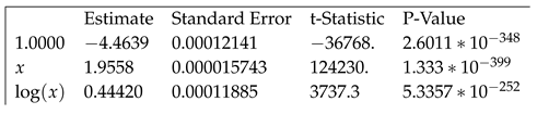
This contribution comes out negative. We fitted these results as (see Figure 6).
Here are the fit statistics
We have the following estimate for the odd N contribution to the enstrophy in the grand canonical Euler ensemble in the local limit:
The leading term grows ; therefore, this correction is negligible.
The enstrophy divergence corresponds to anomalous dissipation in our theory.
This divergence is the dual version of the original anomalous dissipation in the Navier-Stokes velocity field, coming from singular vorticity regions [17,20](Burgers vortexes).
Here, it comes from large fluctuations of the fractal curve in the grand canonical Euler ensemble. These are quantum effects related to the prime factorization of large integers.
4.5. The higher moments of the enstrophy
The higher moments of the distribution of enstrophy are also calculable [29].
We take the point correlation function in the limit of the vanishing loop
With all different , the averaging over the Ising variables is straightforward. It leads to the integral over
This integral is reduced to the hypergeometric function in [26]:
In particular,
This term does not depend on q; it dominates in the local limit at fixed n.
The general formula for the numerator of the moments at fixed N reads
This cotangent sum is reduced to the superposition of multi-totients in Appendix.A
The rational coefficients are given by recurrent relations
The specific cases are considered in Appendix A. We are interested in the local limit, even .
In this limit, the highest totient dominates the sum, and we find for the sum
Finally, in the limit , replacing the sum over even N by of the integral of the asymptotic of this product of gamma functions, we find
These coefficients are all positive. Here are the first five values
4.6. The vorticity distribution
Using the analytic formulas for the moments of the enstrophy, we can study nonperturbative effects in our solution, such as the PDf of the vorticity[29].
Let us consider the Fourier transform of the PDF corresponding to the vorticity moments,
The averaging over the global rotation matrix yields
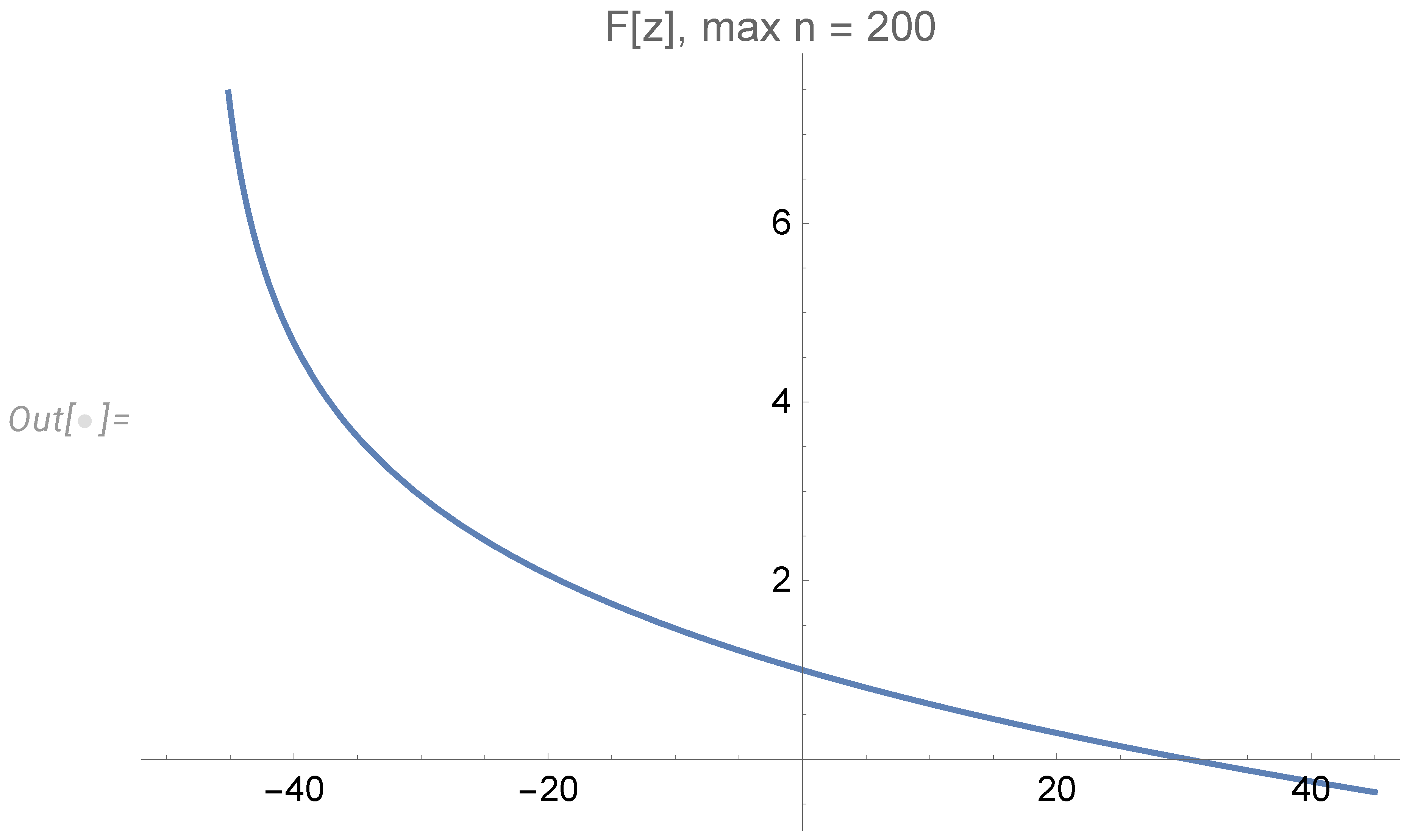
Using our solution for the moments, we get a universal scaling function
This expansion for the scaling function has a finite radius of convergence, as it follows from the asymptotic
The singularity is located at negative . The expansion can be truncated inside the convergence region . Here is the corresponding plot for expansion truncated at (see Figure 7).
At large positive z, it behaves as
This singularity of the Fourier transform at the imaginary axis corresponds to the exponential decrease of the PDF
There is no continuum limit for the distribution of vorticity.
However, this statistical system is renormalizable in the sense that the redefinition of the source
eliminates the singularity in the same way as the redefinition of viscosity
eliminated the singularity in the energy dissipation.
5. The decay index spectrum
The vicinity of the fixed point in nonlinear dynamic systems provides the most interesting physical phenomena, such as anomalous dimensions of various local operators in the theory of renormalization group.
Our system is no exception. Let us perturb the momentum loop equation(21) and study the general properties of this perturbation .
5.1. Linearized loop equation
We get a linearized equation for of the form
These matrices for the decaying solution (41) have an explicit time dependence
which follows from the fact that the RHS of the original loop equation (21) represents the third-degree homogeneous functional of .
We find the linear equation of the form
with being some tensors in . There is no explicit dependence other than through the fixed point solution . We shall write explicit equations in a minute.
This equation has power-like solutions
with the index determined from the eigenvalue problem
We can go one step forward before specifying the parameters of this equation. Let us use our polygonal approximation for . This equation becomes a recurrent equation
We can solve it as a matrix product (in reverse order)
The periodicity requires which leads to the eigenvalue equation (this is already matrix equation)
As a result, we arrive at the spectral equation for the fractal dimensions of decaying turbulence
Here is the explicit form of these two matrices ( with , see [30])
Note that these two matrices are functions of , unlike the fixed point solution (60),(61), where the dependence dropped.
This fact will be important for the distribution of the velocity circulation.
Another important fact. The vector is determined up to total normalization
where the eigenvector is a unit vector, and g is an arbitrary parameter, having dimension
This parameter g is not universal and depends on the initial data specific to the flow, like the energy dissipation in the K41 model.
This issue deserves further numerical and analytical study, which is outside our scope.
5.2. The circulation distribution
The Wilson loop (3) doubles as a Fourier transform of the PDF for the velocity circulation. This PDF can be obtained by inverse Fourier transform
However, substituting the leading term of the solution of the loop equation into this general formula leads to a paradox: this leading term does not depend on . Formally, we get the delta function , which means that this leading term is not sufficient to get the PDF; we need the next correction.
We have found the linear correction to the fixed point, and now we can fix these formulas. Expanding the correction and keeping the leading linear term, we find:
5.3. The spectral identity and Wilson loop asymptotics
The distribution of the eigenvalues can be studied using the resolvent
By construction, at finite N this is a rational function of with simple poles at the spectrum.
In the continuum limit, it becomes a holomorphic function in a complex plane cut along the spectrum.
Consider the clockwise contour surrounding the spectrum of in a complex plane (not necessarily a real axis).
Then, we can use the residue at infinity to compute the contour integral
The left side of this identity can be inserted inside the statistical average, such as the circulation PDF integral (198):
By taking residues in the poles of the resolvent, we can relate this integral to the sum over the spectrum of poles. However, it is better to deform the integration contour to the steepest descent from the saddle point. This contour will allow us an analytic investigation of the large-time asymptotic.
The asymptotic behavior of at a large time t is determined by the saddle point equations for two variables
The stability of our fixed-point solution requires the condition of the saddle point
We plan to study the spectrum of fractal dimensions and asymptotic distribution of the circulation in the forthcoming paper [19], using the NYU AD supercomputer cluster.
6. Discussion
6.1. Singular solutions of the Navier-Stokes equation?
The issue of "finite time singularity" of the Navier-Stokes equation, particularly that without random forcing, has attracted much interest from mathematicians.
The Millennium Prize Problem of proving or disproving the smoothness in the solution of the Navier-Stokes equation remains unsolved.
In our view, the most advanced research in this field so far has been performed by Tao (see his recent review [31]). Based on a simplified model of the averaged Navier-Stokes, Tao conjectured [18] that irregular behavior occurs in finite time.
One of his arguments is based on anomalous dissipation, coming from divergent enstrophy due to singular velocity gradients. The anomalous dissipation occurs only in the vanishing viscosity limit in the Navier-Stokes equation.
We investigated anomalous dissipation in the previous papers [17,20], where we have found the anomalous terms in the Euler Hamiltonian related to the Burgers vortex. This vortex corresponds to a singular Euler solution, with vorticity becoming the delta function at the infinitely thin vortex line in the limit of the Navier-Stokes equation.
In the dual theory developed in this paper, the anomalous dissipation comes from large fluctuations of our fractal curve, leading to divergent enstrophy.
Surprisingly, we have more than anomalous dissipation: the singularity we have found exists at finite viscosity, in a spirit of Tao’s conjecture, though we are not studying a particular solution with a finite time blow-up.
Again, let us stress it: we are not claiming any theorems about finite time singularities of the Navier-Stokes equation. We are studying a different phenomenon: turbulent flow, a stochastic solution of the Navier-Stokes equation, covering a certain manifold.
6.2. Stochastic solution of the Navier-Stokes equation and ergodic hypothesis
We find this manifold (Euler ensemble) by solving the loop equation (a subset of the Hopf functional equation for the generating functional of velocity field probability). None of the particular solutions in this manifold has a finite time blow-up. The singularity emerges from the averaging over the distribution of these solutions over the Euler ensemble.
We take the most natural invariant measure from the point of the number theory: each element of the Euler ensemble enters with equal weight. We call it our ergodic hypothesis.
This hypothesis is not necessary to solve the loop (i.e., Hopf) equation, as any linear superposition of the found solutions would satisfy the loop equation.
The singularities of our Euler grand canonical ensemble at remain in local variables such as enstrophy and its PDF, indicating an intrinsic problem of the Navier-Stokes equation. It has to be regularized at small distances, and viscosity does not provide enough regularization in our solution.
The situation reminds that of the QED in the mid-twentieth century. The continuum limit of the theory showed unexpected divergent integrals due to an infinite number of local degrees of freedom of a continuous electromagnetic field.
In both cases, the continuum theory was an idealization of the real physical system: in the case of QED, there were other forces at small distances, eventually merging QED into the Standard Model, which is still inconsistent at Planck’s ultra-small distances where the quantum gravity enters the game.
In the case of the Navier-Stokes equation, it ignores the molecular structure of fluid. The incompressibility is also an idealization: at large gradients of velocity, the sound waves related to compressibility enter the game, leading to some physical cutoff of infinite vorticity.
In other words, the Navier-Stokes equation has limited applicability in the physical world and needs to be modified at large gradients. After all, this is a phenomenological equation resulting from the truncated expansion of friction forces in velocity gradients.
The common presumption that "viscosity regularizes the velocity field" must be tested beyond the perturbation expansion, which we did in this work.
We present a singular decay solution of the Navier-Stokes loop equations in arbitrary dimension . However, we did not prove that the solution of the Navier-Stokes equation as a PDE with smooth initial data would eventually approach our stochastic solution as an asymptotic regime.
6.3. The physical meaning of the loop equation and dimensional reduction
The long-term evolution of Newton’s dynamical system with many particles eventually covers the energy surface (microcanonical ensemble). The ergodic hypothesis (accepted in Physics but still not proven mathematically) states that this energy surface is covered uniformly.
The Turbulence theory aims to find a replacement of the microcanonical ensemble for the Navier-Stokes equation. This surface would also take part in the decay in the pure Navier-Stokes equation without artificial forcing.
In both cases, Newton and Navier-Stokes, the probability distribution must satisfy the Hopf equation, which follows from the dynamics without specification of the mechanism of the stochastization.
Indeed, the Gibbs, as well as the microcanonical distributions in Newton’s dynamics, satisfy the Hopf equation in a rather trivial way: It reduces to the conservation of the probability measure (Liouville theorem), which suggests the energy surface as the only additive integral of motion to use as a fixed point manifold.
In the case of the decaying turbulence, the loop equations represent a closed subset of the Hopf equations, which are still sufficient to generate the dynamics of vorticity.
In this case, the exact solution we have found for the Hopf functional also follows from the integrals of motion, this time, the conservation laws in the loop space.
The loop space Hamiltonian we have derived from the unforced Navier-Stokes equation does not have any potential terms ( those with explicit dependence upon the shape of the loop).
The Schrödinger equation with only kinetic energy in the Hamiltonian conserves the momentum. The corresponding wave function is the plane wave .
This is the solution we have found, except the dot product becomes a symplectic form in the loop space.
Our momentum is not an integral of motion, but simple scaling properties of the pure Navier-Stokes equation lead to the solution with , with being the integral of motion.
The rest is a purely technical task: substituting this scaling solution into the Navier-Stokes equation and solving the resulting universal equation for a fixed point .
Our solution expresses the probability distribution and expected value for the Wilson loop at any given moment t in terms of an ensemble of fractal loops in complex momentum space. The loop is represented by a polygon with sides.
This statistical system is similar to a one-dimensional Ising ring in an imaginary magnetic field and zero coupling constant. Some global observables, such as the moments of enstrophy, are calculable for arbitrary N as an analytic function of , relating it to the Euler totients and similar functions of the number theory.
The continuum limit differs for odd and even N, which means this limit does not exist. This ambiguity disappears in the grand canonical ensemble.
In this ensemble, the number N of degrees of freedom is not fixed but can also fluctuate, with the weight . These fluctuations smooth out the difference between odd and even ensembles so that the grand canonical ensemble is unambiguous in the continuum limit.
The continuum limit in the grand canonical ensemble corresponds to . In this limit, we compute the partition function (104) and the expectation value of the energy dissipation (147). As discussed in the previous section, the singularities at indicate inconsistencies in the Navier-Stokes equation as an idealization of molecular dynamics.
6.4. Classical flow and quantum geometry
Our computations heavily rely on the number theory, particularly Lehmer’s multitotients , (137), generalizing [27] the Euler totient function.
What could the number theory have in common with the turbulent flow?
The quantization of parameters of the fixed manifold of decaying turbulence stems from the deep quantum correspondence we have discovered. The statistical distribution of a nonlinear classical Navier-Stokes PDE is exactly related to the wave functional of a linear Schrödinger equation in the loop space. The quantization mechanism is the same as in ordinary quantum mechanics: this is a requirement of the periodicity of the solution.
The equivalence of a strong coupling phase of the fluctuating vector field to quantum geometry is a well-known duality phenomenon in gauge theory (the ADS/CFT duality), ringing a bell to the modern theoretical physicist.
In our case, this is a simpler quantum geometry: a fractal curve in complex space.
An expert in the traditional approach to turbulence may wonder why the loop equation’s solutions have any relation to the velocity field’s statistics in a decaying turbulent flow.
Such questions were raised and answered in the last few decades in the gauge theories, including QCD[5,7,8,9] where the loop equations were derived first [3,4]. The short answer is that duality only applies to the correlation functions of two theories with different dynamical variables; there is no correspondence between these variables, but the correlation functions are identical.
Mathematical physics sometimes has alternative languages for the same phenomena; examples are the duality between Schrödinger’s wave equation and Heisenberg’s matrix mechanics, between dynamical triangulation and Liouville theory in 2D quantum gravity.
Extra complications in the gauge theory are the short-distance singularities related to the infinite number of fluctuating degrees of freedom in quantum field theory. The Wilson loop functionals in coordinate space are singular in the gauge field theory and cannot be multiplicatively renormalized.
Perturbatively, there is no short-distance divergence in the Navier-Stokes equations nor the Navier-Stokes loop dynamics. The Euler equations represent the singular limit, which, as we argued, should be resolved using singular topological solitons regularized by the Burgers vortex.
In the present theory, we keep viscosity constant and do not encounter any singularities in coordinate space. The anomalous dissipation is achieved in our solution via a completely different mechanism: large fluctuations of the fractal curve at .
However, we have found the singularity from large vorticity fluctuations at any finite viscosity value. It cannot be attributed to the Euler singularities such as line vortexes. Those vortexes are regularized by finite viscosity, unlike our singularities.
This singularity resembles the conjecture by Tao [18]; however, it has a different meaning. Our singularity is a divergence of correlation functions of vorticity, not the local vorticity as a function of coordinates.
Our vorticity is not a smooth field, developing finite-time singularity at some region of physical space, like a vortex line or a vortex sheet; it is a stochastic field with the singularities (discontinuities) distributed all over the physical space with some multi-dimensional distribution. We compute the correlation functions for this distribution from the dual theory of momentum loop dynamics.
We have divergencies in these correlation functions, like QED, though these divergencies emerge in the exact solution beyond perturbation theory.
6.5. Stokes-type functionals and vorticity correlations
The loop equation describes the gauge invariant sector of the gauge field theory. Therefore, the gauge degrees of freedom are lost in the loop functional. However, the gauge-invariant correlations of the field strength are recoverable from the solutions of the loop equation[3,4].
There is no gauge invariance regarding the velocity field in fluid dynamics (though there is such invariance in the Clebsch variables [17]). The longitudinal, i.e., a potential part of the velocity, has a physical meaning – it is responsible for pressure and energy pumping. This part is lost in the loop functional but is recoverable from the rotational part (the vorticity) using the Biot-Savart integral.
In the Fourier space, the correlation functions of the velocity field are algebraically related to those of vorticity . Thus, the general solution for the Wilson loop functional allows computing both vorticity and velocity correlation functions.
We demonstrated that in the last two sections by computing the moments of the enstrophy and resulting anomalous dissipation. This computation is nonperturbative: it corresponds to the extreme turbulent limit and cannot be expanded in inverse powers of viscosity.
6.6. Relation of our solution to the weak turbulence
The solution of the loop equation with finite area derivative, satisfying Bianchi constraint, belongs to the so-called Stokes-type functionals [3], the same as the Wilson loop for Gauge theory and fluid dynamics.
The Navier-Stokes Wilson loop is a case of the Abelian loop functional, with commuting components of the vector field .
As we discussed in detail in [3,4,17], any Stokes-type functional satisfying boundary condition at shrunk loop , and solving the loop equation can be iterated in the nonlinear term in the Navier-Stokes equations (which iterations would apply at large viscosity).
The resulting expansion in inverse powers of viscosity (weak turbulence) exactly coincides with the ordinary perturbation expansion of the Navier-Stokes equations for the velocity field, averaged over the distribution of initial data or boundary conditions at infinity.
We have demonstrated in [2,17] (and also here, in Section 1.3) how the velocity distribution for the random uniform vorticity in the fluid was reproduced by a singular momentum loop .
The solution for in this special fixed point of the loop equation was random complex and had slowly decreasing Fourier coefficients, leading to a discontinuity in a pair correlation function (35). The corresponding Wilson loop was equal to the Stokes-type functional (27).
Using this example, we demonstrated how a discontinuous momentum loop describes the vorticity distribution in the stochastic Navier-Stokes flow. In this example, the vorticity is a global random variable corresponding to a random uniform fluid rotation: a well-known exact solution of the Navier-Stokes equation.
This example corresponds to a special fixed point for the loop equation, not general enough to describe the turbulent flow but mathematically ideal as a toy model for the loop technology. It demonstrates how the momentum loop solution sums up all the terms of the expansion in the Navier-Stokes equation.
In our general solution, with the Euler ensemble, the summation of a divergent perturbation expansion occurs at an extreme level, leading to a universal fixed point independent of viscosity. At a given initial condition, after a finite time, the solution will still depend on viscosity and initial condition.
At large time, though, it will approach our universal fixed manifold and (supposedly, for random initial data) cover it uniformly, according to the Euler ensemble measure.
The vorticity will become a random variable with a singular distribution in the local limit, suggesting intrinsic inconsistency of the Navier-Stokes equation.
6.7. Continuum spectrum of anomalous dimensions and multifractality
We studied the linear perturbations of our fixed manifold, which decay with time as , with a calculable spectrum of decay indexes . At fixed parameters of the Euler ensemble, this spectrum is discrete, but with random values of these parameters, in the local limit , the spectrum becomes continuous.
The explicit equation (192) for the spectrum of anomalous dimensions in decaying turbulence is a nice surprise. Future investigation will likely relate it to some multifractal properties.
We derived the representation for the averages over this continuum spectrum for the Wilson loop PDF (204).
This kind of saddle point integral is used to justify the multifractal models. In our case, the weight in that integral is calculable in terms of the Euler ensemble. The analytic result for the large-time asymptotic would require more work, however.
The most urgent task is to study the stability of our spectrum of decay indexes . We do not see any alternative to numerical study of this spectrum [19].
6.8. Conclusion
The exact solution for in decaying turbulence, which we have found in this paper, leads to the Stokes functional satisfying the boundary value at the shrunk loop.
Therefore, it describes a stochastic Navier-Stokes flow, corresponding to the degenerate fixed point of the Hopf equation for the generating functional of velocity circulation.
It sums up all the Wylde diagrams in the limit of vanishing random forces plus nonperturbative effects, which are missed in the Wylde functional integral, particularly the quantization of parameters of the solution.
These quantum effects follow from the exact equivalence of the Navier-Stokes statistics to the quantum mechanics in loop space [2].
The most striking nonperturbative effect is the singularity of vorticity distribution in the local limit for a finite viscosity.
Compared to the other critical phenomena, this theory is amazingly simple: It is not a field theory but a discrete statistical system similar to the one-dimensional Ising ring in the presence of the imaginary quantized magnetic field.
Still, the solution is far from trivial and reveals unexpected relations between turbulence and number theory. In particular, the anomalous energy dissipation constant (148) is related to the prime factorization of large integers used in so-called multi-totients [27].
Whether this quantum solution to the classical problem is realized in Nature remains to be seen.
Data Availability Statement
Acknowledgments
I benefited from discussions of this theory with Sasha Polyakov, K.R. Sreenivasan, Peter Sarnak, Tristan Buckmaster, Greg Eyink, Luca Moriconi, Vladimir Kazakov, Kartik Iyer, and Maxim Bulatov. Maxim helped me compute the number theory function , used in the enstrophy’s local limit (to be published in [19]).
This research was supported by a Simons Foundation award ID 686282 at NYU Abu Dhabi.
Appendix A. Euler averages as multitotient functions
The Euler ensemble expectation value of can be reduced to the prime numbers as follows. We start with an unconstrained sum, which is elementary [26].
Let us consider a sum of arbitrary function constrained to the coprime . In our case
Such sum satisfies the following equation (with denoting S ordered prime factors of m and denoting coprime ).
Let us go into detail. Consider the first term for particular
We observe that the second term removes from the total sum in the first term all the terms with . In the same way, the other terms in the sum remove all the terms in the first sum with .
However, there are terms in like , which are proportional to two prime factors , and we removed these terms twice, once in the term and the second time in .
So, we have to add them back, with sign for each pair . This addition provides the next term with double sum .
In general, this formula is a particular case of the inclusion-exclusion principle [35].
As the basic equation (A6) is a linear functional of H, we can solve this equation separately for , and then by adding these solutions with proper coefficients, we get the solution for our particular .
Let us start with the simplest case, . The solution is the Euler . Here is how the equation is satisfied:
The next case, is processed the same way, with the result
Finally, the function
Putting all together
These multitotients were introduced by Lehmer in 1900 [27].
The asymptotic behavior of the multitotient summators was computed in that paper:
We also need similar sum rules for higher powers of .
This sum belongs to the general category of the sums with
Repeating the above arguments, we only need to know the polynomial expansion of the unconstrained sum of the power of cotangent. This sum was computed in [36]. The expression in that paper contained a n-fold sum and thus was hard to use in any analytic or numerical computation.
We reduced this multiple sum to the following linear recurrent equation (with being the Bernoulli coefficients)
The coefficients of the cotangent sum are related to these coefficients BernSum as follows
This recurrent equation is easily solved for any finite n and, being linear, can also be analyzed in the limit of large n. Here are the first four sums
The last step is to replace the powers of m with corresponding multitotients, according to the above theory
Note that the term without a power of m dropped as . Here are the first four sums
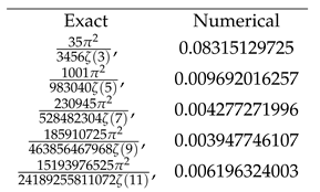
The Mathematica®does not know how to simplify the sums like for , but we can use it to numerically compute these sums and compare them with our totient solution. Here is an example for
 Only the first 10 digits out of the requested 20 came out correct with numerical evaluation.
The real advantage of the exact solution is that its computational complexity grows only logarithmically with m, at least for the achievable values where the prime factorization does not present a problem.
The original definition with the sum over comprime has a linear complexity.
References
- Migdal, A.A. Random Surfaces and Turbulence. In Proceedings of the International Workshop on Plasma Theory and Nonlinear and Turbulent Processes in Physics, Kiev, April 1987; Bar’yakhtar, V.G., Ed. World Scientific, 1988, p. 460.
- Migdal, A. Loop Equation and Area Law in Turbulence. In Quantum Field Theory and String Theory; Baulieu, L.; Dotsenko, V.; Kazakov, V.; Windey, P., Eds.; Springer US, 1995; pp. 193–231. [CrossRef]
- Makeenko, Y.; Migdal, A. Exact equation for the loop average in multicolor QCD. Physics Letters B 1979, 88, 135–137. [Google Scholar] [CrossRef]
- Migdal, A. Loop equations and 1N expansion. Physics Reports 1983, 201. [Google Scholar] [CrossRef]
- Migdal, A. Momentum loop dynamics and random surfaces in QCD. Nuclear Physics B 1986, 265, 594–614. [Google Scholar] [CrossRef]
- Migdal, A. Second quantization of the Wilson loop. Nuclear Physics B - Proceedings Supplements 1995, 41, 151–183. [Google Scholar] [CrossRef]
- Migdal, A.A. Hidden symmetries of large N QCD. Prog. Theor. Phys. Suppl. 1998, 131, 269–307. [Google Scholar] [CrossRef]
- Anderson, P.D.; Kruczenski, M. Loop equations and bootstrap methods in the lattice. Nuclear Physics B 2017, 921, 702–726. [Google Scholar] [CrossRef]
- Kazakov, V.; Zheng, Z. Bootstrap for lattice Yang-Mills theory. Phys. Rev. D 2023, arXiv:hep-th/2203.11360]107, L051501. [Google Scholar] [CrossRef]
- Ashtekar, A. New variables for classical and quantum gravity. Physical Review Letters 1986, 57, 2244–2247. [Google Scholar] [CrossRef]
- Rovelli, C.; Smolin, L. Knot Theory and Quantum Gravity. Phys. Rev. Lett. 1988, 61, 1155–1158. [Google Scholar] [CrossRef] [PubMed]
- Iyer, K.P.; Sreenivasan, K.R.; Yeung, P.K. Circulation in High Reynolds Number Isotropic Turbulence is a Bifractal. Phys. Rev. X 2019, 9, 041006. [Google Scholar] [CrossRef]
- Iyer, K.P.; Bharadwaj, S.S.; Sreenivasan, K.R. The area rule for circulation in three-dimensional turbulence. Proceedings of the National Academy of Sciences of the United States of America 2021, 118, e2114679118. [Google Scholar] [CrossRef]
- Apolinario, G.; Moriconi, L.; Pereira, R.; valadão, V. Vortex Gas Modeling of Turbulent Circulation Statistics. PHYSICAL REVIEW E 2020, 102, 041102. [Google Scholar] [CrossRef]
- Müller, N.P.; Polanco, J.I.; Krstulovic, G. Intermittency of Velocity Circulation in Quantum Turbulence. Phys. Rev. X 2021, 11, 011053. [Google Scholar] [CrossRef]
- Parisi, G.; Frisch, U. On the singularity structure of fully developed turbulence Turbulence and Predictability. In Proceedings of the Geophysical Fluid Dynamics: Proc. Intl School of Physics E. Fermi; M Ghil, R.B.; Parisi, G., Eds. Amsterdam: North-Holland, 1985, pp. 84–88.
- Migdal, A. Statistical Equilibrium of Circulating Fluids. Physics Reports 2023, arXiv:physics.flu-dyn/2209.12312]1011C, 1–117. [Google Scholar] [CrossRef]
- Tao, T. Finite time blowup for an averaged three-dimensional Navier-Stokes equation. Journal of the American Mathematical Society 2016, 29, 601–674. [Google Scholar] [CrossRef]
- Maxim Bulatov, A.M. Numerical Simulations of Fractal Curve in Decalying Turbulence Theory. to be submitted to Fractal and Fractions.
- Migdal, A. Topological Vortexes, Asymptotic Freedom, and Multifractals. MDPI Fractals and Fractional, Special Issue 2023, [arXiv:physics.flu-dyn/2212.13356]. arXiv:physics.flu-dyn/2212.13356]. [CrossRef]
- Migdal, A. Symmetric Fixed Point. https://www.wolframcloud.com/obj/sasha.migdal/Published/SymmetricFixedPoint.nb, 2023.
- Gross, D.J.; Migdal, A.A. Nonperturbative two-dimensional quantum gravity. Phys. Rev. Lett. 1990, 64, 127–130. [Google Scholar] [CrossRef]
- AGISHTEIN, M.; MIGDAL, A. SIMULATIONS OF FOUR-DIMENSIONAL SIMPLICIAL QUANTUM GRAVITY AS DYNAMICAL TRIANGULATION. Modern Physics Letters A 1992, 07, 1039–1061. [Google Scholar] [CrossRef]
- Wikipedia contributors. Euler’s totient function — Wikipedia, The Free Encyclopedia. https://en.wikipedia.org/w/index.php?title=Euler%27s_totient_function&oldid=1163400966, 2023. [Online; accessed 6-August-2023].
- Basak, D.; Zaharesku, A. Euler ensemble for the odd case. private communication, to be published.
- Migdal, A. Enstrophy Computations. https://www.wolframcloud.com/obj/sasha.migdal/Published/Enstrophy.
- Lehmer, D.N. Asymptotic Evaluation of Certain Totient Sums. American Journal of Mathematics 1900, 22, 293–335. [Google Scholar] [CrossRef]
- Migdal, A. Sum Cotangent Squared. https://www.wolframcloud.com/obj/sasha.migdal/Published/TestMultitotients.nb, 2023.
- Migdal, A. Moments of Vorticity. https://www.wolframcloud.com/obj/sasha.migdal/Published/Momets.
- Migdal, A. Multifractal Spectrum. https://www.wolframcloud.com/obj/sasha.migdal/Published/MultifractalSpectrum.nb, 2023.
- Tao, T. Searching for singularities in the Navier–Stokes equations. Nature Reviews Physics 2019, 1, 418–419. [Google Scholar] [CrossRef]
- Migdal, A. Corr Function Integrals. https://www.wolframcloud.com/obj/sasha.migdal/Published/CorrFunctionIntegrals.nb, 2023.
- Migdal, A. Analytic Solution for Enstrophy. https://www.wolframcloud.com/obj/sasha.migdal/Published/AnalyticSolutionEnstrophy.nb, 2023.
- Migdal, A. Euler Partition Function. https://www.wolframcloud.com/obj/sasha.migdal/Published/EnstrophyEuler.nb, 2023.
- Wikipedia contributors. Inclusion–exclusion principle — Wikipedia, The Free Encyclopedia. https://en.wikipedia.org/w/index.php?title=Inclusion%E2%80%93exclusion_principle&oldid=1170123427, 2023. [Online; accessed 22-August-2023].
- Franke, J. Rational functions, cotangent sums and Eichler integrals. Research in Number Theory 2021, 7, 23. [Google Scholar] [CrossRef]
Figure 1.
Log-log plots of four ratios for even/odd , even/odd . The larger N led to astronomically small ratios, so we did not use them.
Figure 1.
Log-log plots of four ratios for even/odd , even/odd . The larger N led to astronomically small ratios, so we did not use them.
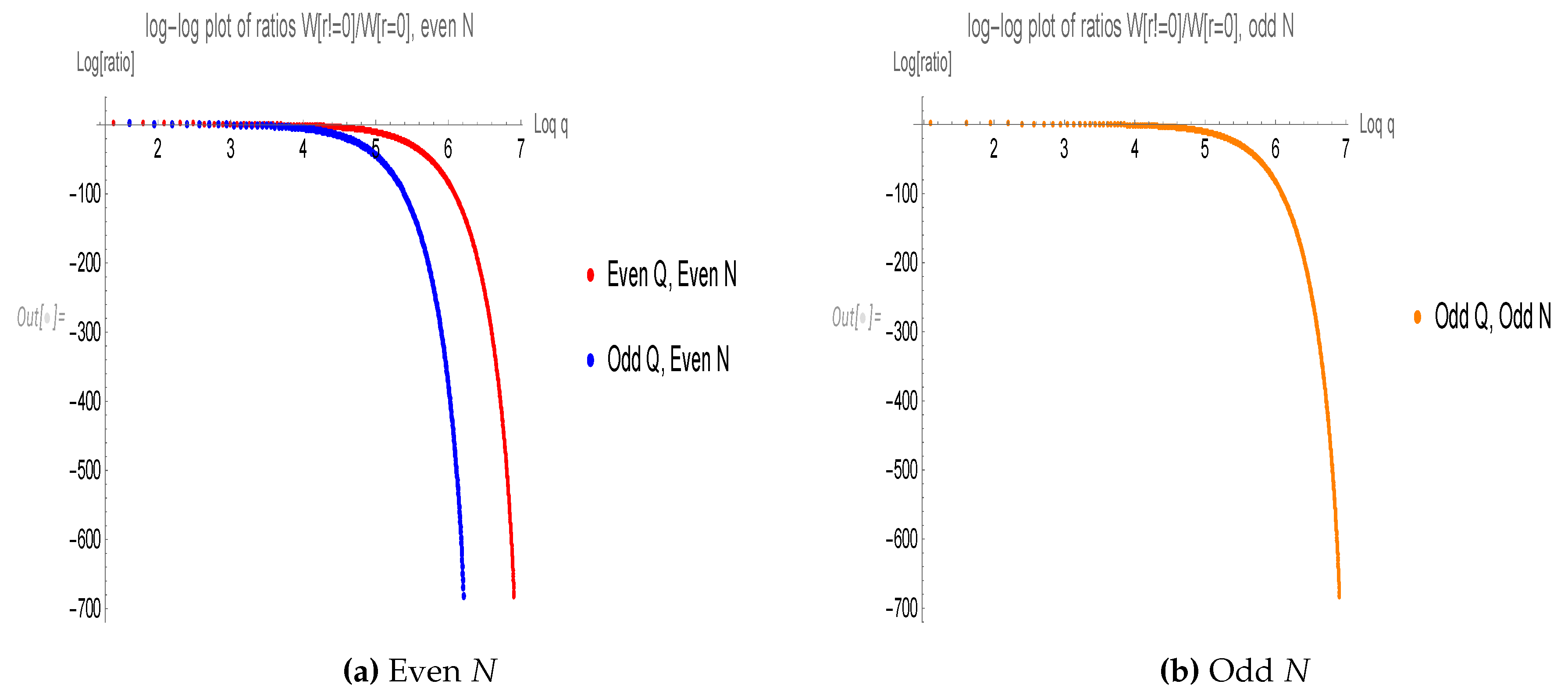
Figure 2.
Partition function for odd N, fitted as
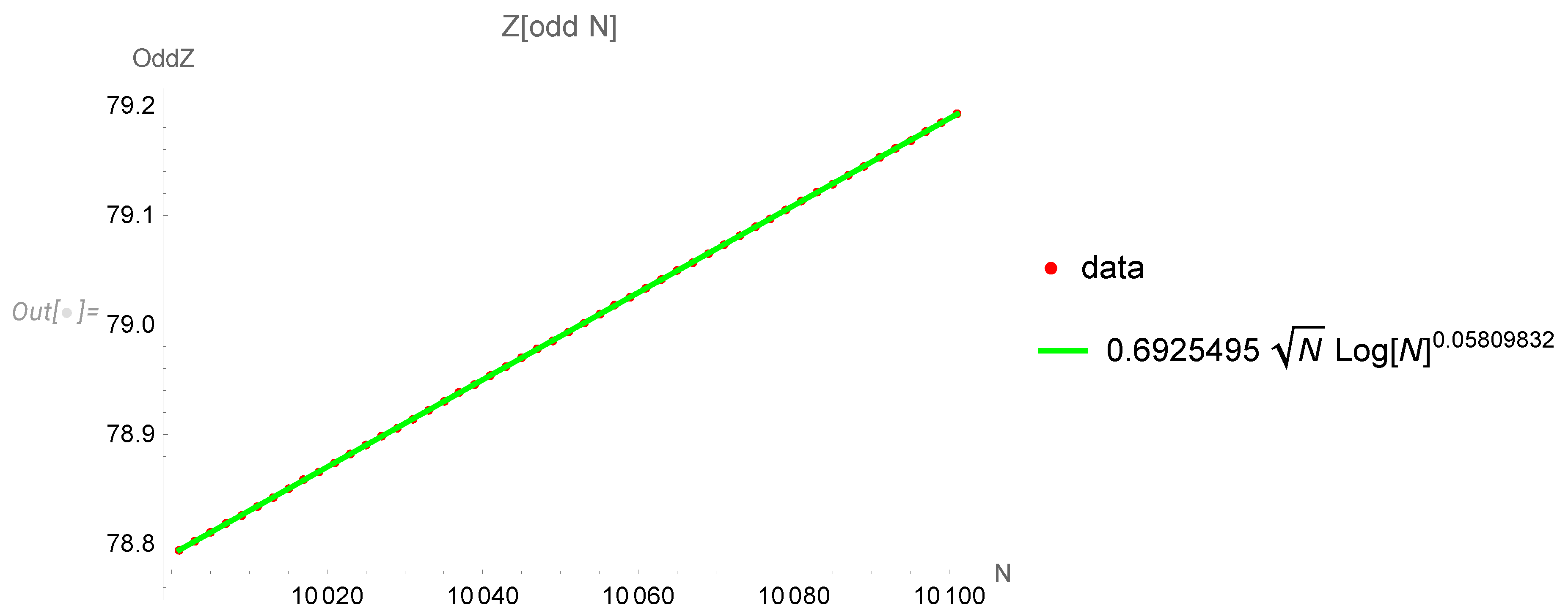
Figure 3.
Backtracking wires corresponding to vorticity correlation function.
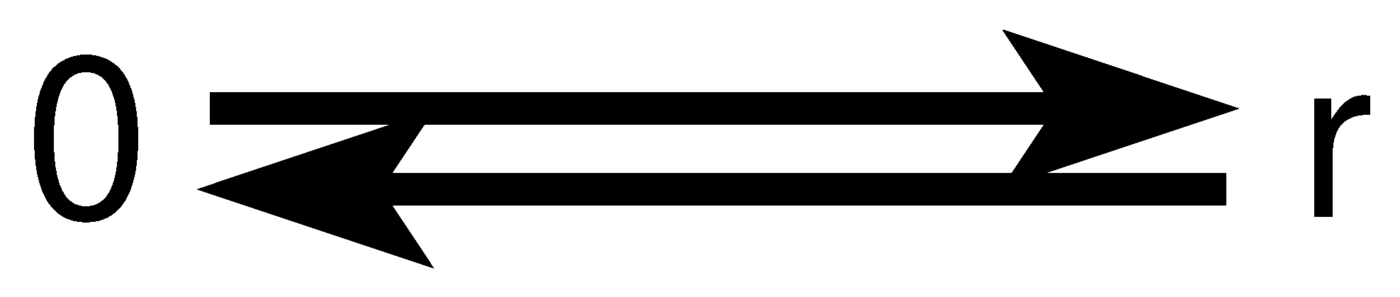
Figure 4.
The relative variance computed in the text in the statistical limit.
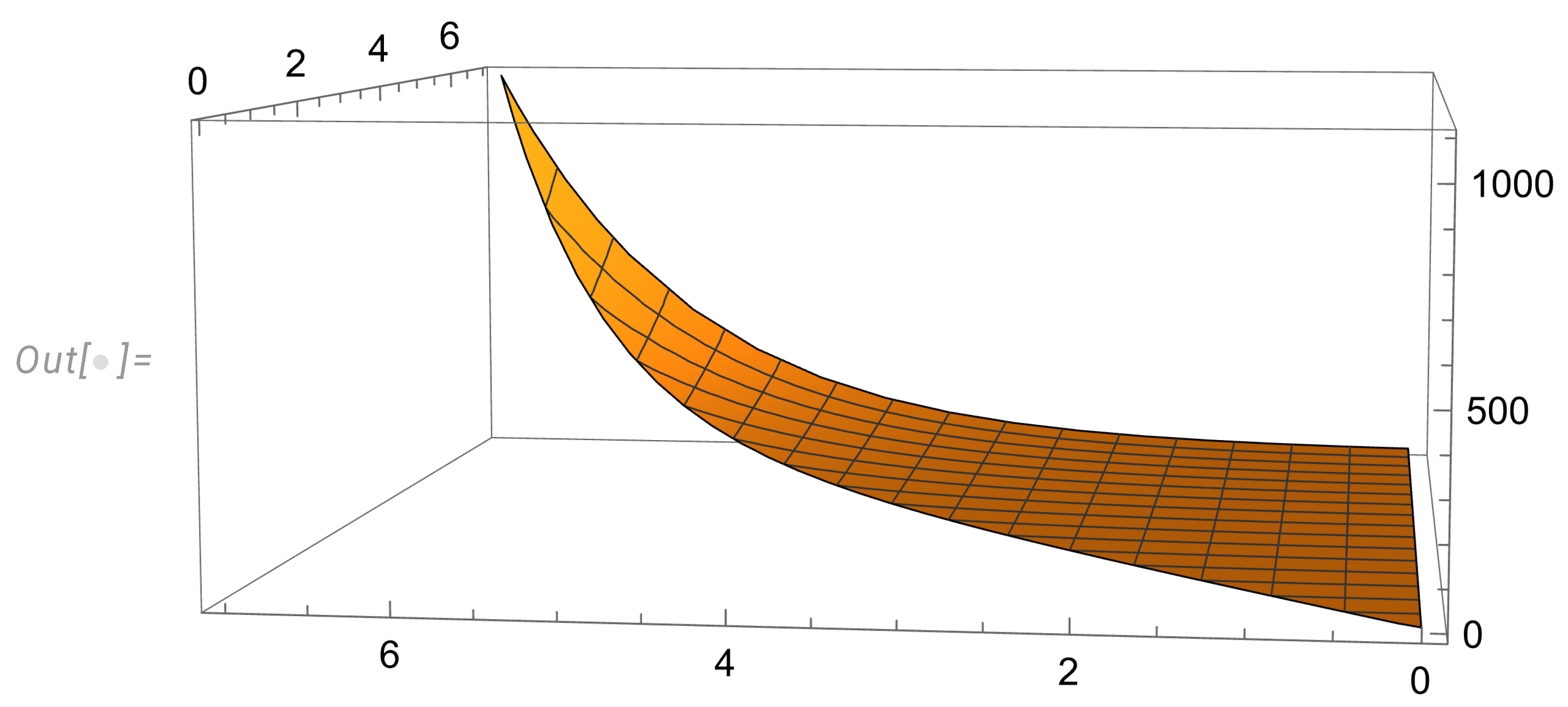
Figure 5.
S(q) for . It does not reach any smooth limit; several bands persist up to infinity, similar to the Euler totient .
Figure 5.
S(q) for . It does not reach any smooth limit; several bands persist up to infinity, similar to the Euler totient .
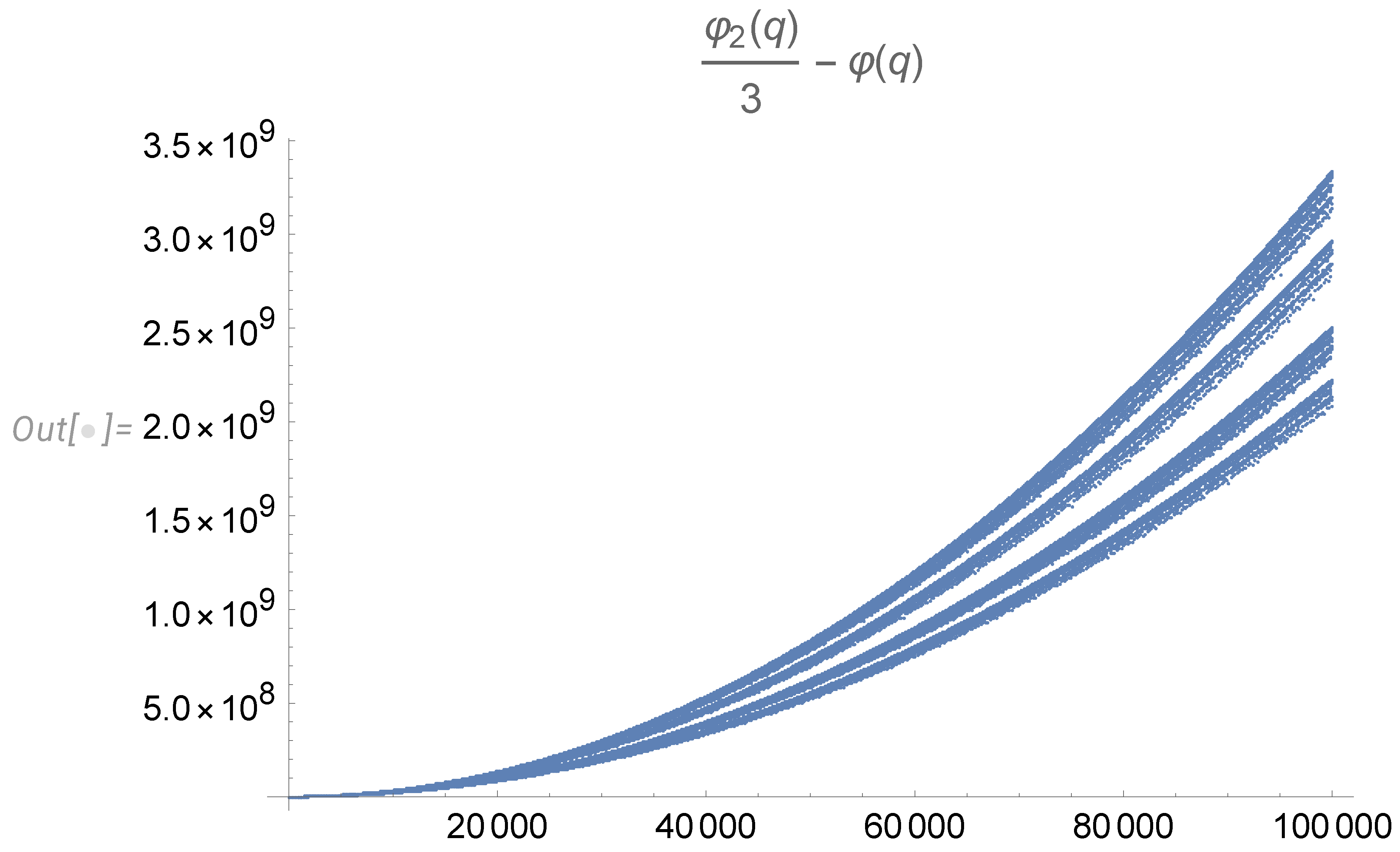
Figure 6.
The direct computation of the odd N contribution to the enstrophy with 20 digits fitted as .
Figure 6.
The direct computation of the odd N contribution to the enstrophy with 20 digits fitted as .
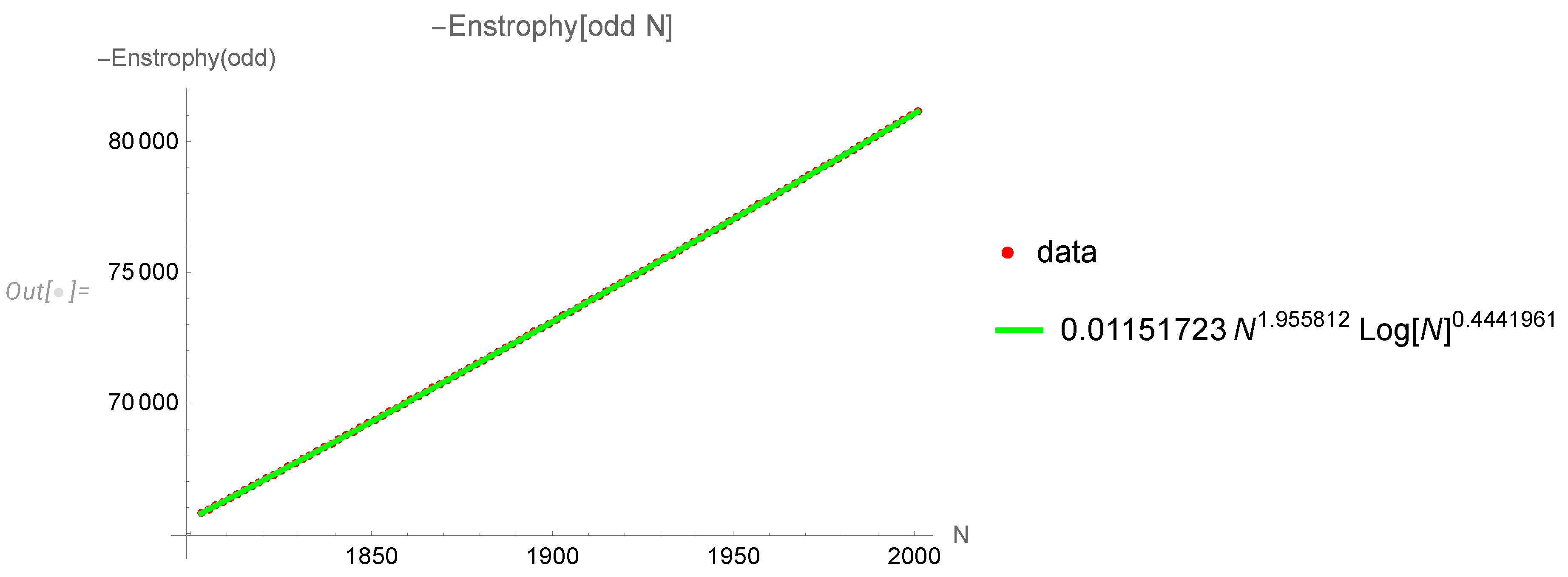
Figure 7.
The scaling function , truncated at .
Disclaimer/Publisher’s Note: The statements, opinions and data contained in all publications are solely those of the individual author(s) and contributor(s) and not of MDPI and/or the editor(s). MDPI and/or the editor(s) disclaim responsibility for any injury to people or property resulting from any ideas, methods, instructions or products referred to in the content. |
© 2023 by the authors. Licensee MDPI, Basel, Switzerland. This article is an open access article distributed under the terms and conditions of the Creative Commons Attribution (CC BY) license (http://creativecommons.org/licenses/by/4.0/).
Copyright: This open access article is published under a Creative Commons CC BY 4.0 license, which permit the free download, distribution, and reuse, provided that the author and preprint are cited in any reuse.


