Submitted:
23 August 2023
Posted:
25 August 2023
You are already at the latest version
Abstract
Diabetes mellitus is a widespread chronic metabolic disorder demanding regular blood glucose level surveillance (BGLs). Current invasive techniques, such as finger-prick tests, often result in discomfort for patients, leading to infrequent monitoring and potential health complications. The primary objective of this study was to design a novel, portable, non-invasive system for diabetes detection using breath samples, named as DiabeticSense, an affordable digital health device for early detection, encouraging immediate intervention. The device employed MOSFET-based electrochemical sensors to assess volatile organic compounds in breath samples, whose concentrations differ between diabetic and non-diabetic individuals. The system merged body vital signs with sensor voltages obtained by processing breath sample data to predict diabetic conditions. Our research used readings from 100 patients at a nationally recognised hospital to form the dataset. Data was then processed 10 using a Gradient Boosting Classifier model, and performance was cross-validated. The proposed system attained a promising accuracy of 86.6%, marking an improvement of 20.72% over an existing regression technique. The developed device introduces a non-invasive, cost-effective, and user-friendly solution for preliminary diabetes detection. It has the potential to increase patient adherence to regular monitoring.
Keywords:
digital health devices
; diabetes test
; bio-markers
; blood glucose monitoring
; diabetes
; exhaled breath analysis
; non-invasive
; volatile organic compounds
1. Introduction
Type-2 Diabetes Mellitus (T2DM) is a chronic metabolic disorder with high blood sugar levels (hyperglycemia). It is caused by either inadequate insulin production by the pancreas or the body’s inability to effectively use the insulin produced, a condition known as insulin resistance [1]. The International Diabetes Federation (IDF) and World Health Organization (WHO) report approximately 500 million T2DM cases worldwide and estimate it to rise to around 800 million by 2045 [2,3]. T2DM, if left untreated or ignored, can lead to serious health complications, including damage to the eyes, blood vessels, kidneys, nerves, heart, and feet. These complications can lead to long-term disability and premature death. According to the World Health Organization (WHO), an estimated 1.6 million deaths were directly attributed to diabetes in 2019, making it the seventh leading cause of mortality worldwide. Moreover, the burden of undiagnosed cases (46.1%) remains alarmingly high, with many individuals being diagnosed only at advanced stages. In India, for instance, approximately 101 million people are already diagnosed with diabetes, and 136 million are in the pre-diabetic stages, highlighting the urgent need for early detection and intervention.
Electronic noses comprising electronic sensors capable of smell or odour detection have found their application in various areas such as food, wine, material, tea, environment, and healthcare. In particular, their ability to discern subtle variations in scent profiles has opened up exciting possibilities for improving diagnostics and disease monitoring. For example, research has shown that the concentration of certain VOCs differs significantly in diabetic individuals compared to non-diabetic individuals [4]. This is because VOCs are produced by the body as a byproduct of metabolism, and their levels can be affected by a variety of factors, including disease.
Electronic sensors that are sensitive to specific VOCs can be used to detect these changes in breath and potentially provide early warning of disease. For example, a study showed that an electronic nose could be used to distinguish between diabetic and non-diabetic individuals with an accuracy of 90% [5]. This is a promising development, as current methods for diagnosing diabetes, such as finger-prick tests, can be invasive and uncomfortable for patients, leading to infrequent monitoring and potential health complications [6,7]. Electronic noses could provide a more non-invasive and convenient way to monitor blood sugar levels and detect diabetes early, which could lead to better health outcomes. Also, the existing non-invasive methods are mainly based on breath simulation data [8] and probabilistic estimation techniques [9]. To the best of our knowledge, there exist few (or none) non-invasive diabetes detection systems that are capable of detecting diabetes from breath using electronic sensors.
Therefore, to bridge the current gap in literature, we propose a portable, non-invasive device for diabetes detection using breath, named as DiabeticSense, incorporating cutting-edge MOSFET-based electrochemical sensors capable of detecting VOCs in a patient’s breath. Leveraging this unique biomarker pattern of a diabetic person, our non-invasive diabetes detection system offers an excellent pre-diagnostic tool for identifying diabetes at its early stage. The portability and affordability of our device make it particularly suitable for deployment in remote health centres, where access to comprehensive medical facilities may be limited. By providing a convenient and user-friendly alternative to traditional invasive tests, our non-invasive diabetes detection device empowers healthcare professionals in resource-constrained settings to perform timely and accurate diabetes screenings.
In this paper, we present the development and methodology of our non-invasive diabetes detection device, along with its promising performance in detecting diabetes. Additionally, we discuss the potential implications of this breakthrough technology in enhancing diabetes management and improving overall health outcomes, particularly in regions where early detection can significantly impact disease progression and reduce diabetes-related complications.
2. Background
The idea of non-invasive glucose monitoring has been a focal point in diabetes care, aiming to replace or reduce the traditional invasive methods. Breath-based analysis, which detects volatile organic compounds (VOCs) indicative of glucose metabolism, stands out due to its promise. Machine learning (ML) algorithms enhance this approach as computational methods advance, offering precise pattern recognition from complex breath samples.
The correlation between specific VOCs in human breath and blood glucose levels has been known for a while. For instance, breath acetone has been identified as a pivotal biomarker for Type 2 diabetes, directly linked with blood glucose concentrations [10,11]. However, more is needed to know how the complete breath, which includes a combination of VOCs, can represent glucose levels.
With the proliferation of smartphone technology, digital interventions have become instrumental in diabetic care. Applications providing diabetes coaching have been introduced to prevent the onset of complications and bolster diabetes self-management. A notable study exemplified how a smartphone application can substantially aid diabetes intervention [12]. Similarly, the impact of a smartphone application is assessed on the self-management of adults with type 1 diabetes, emphasising the integral role such applications play in contemporary diabetes care [13]. However, both studies were limited by the small sample size and the short duration of the intervention.
Furthermore, advancements in sensor technology, particularly the development of Electronic Nose (E-Nose) systems, have significantly enhanced the specificity and sensitivity of VOC detection. Such systems have been crucial in medical domains and have even found applications in identifying cigarette brands, emphasising their versatility and wide-ranging potential [4,9,14,15] and emphasising the feasibility of non-invasive blood glucose monitoring through breath signal analysis. However, there is a need to test these systems for blood glucose monitoring via breath thoroughly. For example, authors in [8] highlighted the development of a human breath analysis system employing solid-state electrochemical sensors based on a digital nose framework. In addition to that, it is evident from the study that the diverse variety of breath components necessitates the utilisation of an artificial intelligence-driven predictive methodology. However, the approaches for optimal power management to handle thermal aspects of the device for high-efficiency performance were yet to be explored for specific use cases. Similarly, authors in [16] showed the significance of power efficiency in output voltage regulation provided by switching regulators. However, the study highlighted the concern regarding undesirable ripples in switching regulators that might hinder the high-performance operation of embedded systems.
ML models have been employed to harness breath data for diabetes detection. Their application demonstrates a high degree of accuracy and underscores the expansive potential of computational methods in medical diagnostics [8]. The versatility of these models is further evidenced by their applicability to diverse datasets, as seen with the Chinese diabetes datasets [17].
Despite these advancements, there remains an observable gap. While there’s growing research on breath-based glucose monitoring and ML for medical diagnostics, literature remains sparse regarding synthesising a comprehensive array of sensors for breath sampling with auxiliary physiological parameters, such as blood pressure, age, gender, and SpO levels. Integrating these would potentially refine predictive accuracy, signifying an area yet to be extensively explored.
DiabeticSense proposed in this research overcomes several limitations in the existing literature. Specifically, it considers a plurality of VOCs the device with proper filter and power management along with ensemble ML algorithms for the classification of diabetes.
3. Materials and Methods
3.1. Study Aim
To develop and evaluate a low-cost portable, non-invasive multi-sensor diabetes detection device (named as DiabeticSense) that uses breath samples and body vitals as input and generates diabetes predictions based on ML models.
3.2. Design
DiabeticSense (Figure 1a) comprises a sensor array of various MOSFET-based electrochemical sensors arranged in a cylindrical manner integrated into a soda sipper cup with a tightly closing cap (Figure 1b). We use birthday balloons to collect breath samples, and a drip pipe (Figure 1c) to infuse the breath sample slowly into our device.
The specifics of the sensors employed are outlined in Table 1. These sensors were meticulously linked to a microcontroller via a 16-bit analogue-to-digital converter (ADC), specifically the ADS1115. The interfacing between the microcontroller and the ADS1115 was facilitated by utilising the I2C communication protocol. To facilitate network interaction, a WIFI-enabled ESP32 microcontroller is used in this experiment. Communication between the microcontroller and external entities was effectuated by utilising the MQTT protocol, establishing a link with a remote MQTT server within the network. The streaming of MQTT-derived data was channeled into an InfluxDB1 time series database. For the visualisation and comprehensive examination of the device’s response, the InfluxDB was managed and visually represented using the Grafana tool2. This enabled insightful analysis of the device’s performance.
3.3. Details of Sensors Used
- TGS 826: The sensing element of TGS826 is a metal oxide semiconductor that has low conductivity in clean air. In the presence of a detectable gas, the sensor’s conductivity increases depending on the gas concentration in the air. A simple electrical circuit can convert the change in conductivity to an output signal corresponding to the gas concentration. The TGS826 has a high sensitivity to ammonia gas. The sensor can detect concentrations as low as 30 ppm in the air and is ideally suited to critical safety-related applications such as the detection of ammonia leaks in refrigeration systems and ammonia detection in the agricultural field [18].
- TGS 2610: TGS2610 is a semiconductor-type gas sensor that combines very high sensitivity to LP gas with low power consumption and long life. Due to the miniaturisation of its sensing chip, TGS2610 requires a heater current of only 56mA and the device is housed in a standard TO-5 package. The TGS2610 is available in two different models with different external housings but identical sensitivity to LP gas. Both models can satisfy the requirements of performance standards such as UL1484 and EN50194. TGS2610-C00 possesses a small size and quick gas response, making it suitable for gas leakage checkers. TGS2610-D00 uses filter material in its housing, eliminating the influence of interference gasses such as alcohol, resulting in a highly selective response to LP gas. This feature makes the sensor ideal for residential gas leakage detectors, which require durability and resistance against interference gas [19].
- TGS 822: The sensing element of 822 Figaro gas sensors is a tin dioxide (SnO2) semiconductor with low conductivity in clean air. In the presence of a detectable gas, the sensor’s conductivity increases depending on the gas concentration in the air. A simple electrical circuit can convert the change in conductivity to an output signal corresponding to the gas concentration. The TGS 822 is highly sensitive to the vapours of organic solvents and other volatile vapours. It also sensitive to combustible gasses such as carbon monoxide, making it an excellent general-purpose sensor. Also available with a ceramic base that is highly resistant to severe environments as high as 200°C (in TGS 823) [20].
- TGS 2602: The sensing element consists of a metal oxide semiconductor layer formed on the alumina substrate of a sensing chip together with an integrated heater. The TGS 2602 is highly sensitive to low concentrations of odourous gasses such as ammonia and HS generated from waste materials in office and home environments. The sensor also susceptible to low concentrations of VOCs, such as toluene emitted from wood finishing and construction products. Due to the miniaturisation of the sensing chip, TGS 2602 requires a heater current of only 56mA and the device is housed in a standard TO-5 package [21].
- TGS 2600: The sensing element consists of a metal oxide semiconductor layer formed on an alumina substrate of a sensing chip together with an integrated heater. In the presence of a detectable gas, the sensor’s conductivity increases depending on the gas concentration in the air. The TGS 2600 is highly sensitive to low concentrations of gaseous air contaminants in cigarette smoke, such as hydrogen and carbon monoxide. The sensor can detect hydrogen at a level of several ppm. Due to the miniaturisation of the sensing chip, TGS 2600 requires a heater current of only 42mA and the device is housed in a standard TO-5 package [22].
- TGS 2603: The sensing element consists of a metal oxide semiconductor layer formed on an alumina substrate of a sensing chip together with an integrated heater. In the presence of a detectable gas, the sensor’s conductivity increases depending on the gas concentration in the air. The TGS 2603 is highly sensitive to low concentrations of odourous gasses such as anime-series and sulfurous odour generated from waste materials or spoiled foods such as fish. By utilising the change ratio of sensor resistance from the resistance in clean air as the relative response, human perception of air contaminants can be simulated and practical air quality control can be achieved [23].
- TGS 2620: The sensing element consists of a metal oxide semiconductor layer formed on an alumina substrate of a sensing chip together with an integrated heater. In the presence of a detectable gas, the sensor’s conductivity increases depending on the gas concentration in the air. The TGS 2620 is highly sensitive to the vapours of organic solvents and other volatile vapours, making it suitable for organic vapour detectors/alarms. Due to the miniaturisation of the sensing chip, TGS 2620 requires a heater current of only 42mA and the device is housed in a standard TO-5 package [24].
- MQ138: The sensor measures the change in conductivity of a tin dioxide SnO semiconductor when exposed to VOCs. In clean air, SnO has low conductivity. However, when VOCs are present, they react with the SnO and increase its conductivity. The change in conductivity can be measured as a voltage change, which can then be used to determine the concentration of VOCs in the air. The MQ138 sensor is sensitive to various of VOCs, including formaldehyde, benzene, toluene, and acetone. It has a working range of 1 to 100 ppm for benzene [25].
- DHT 22: DHT22 is a commonly used temperature and humidity sensor. The sensor comes with a dedicated NTC to measure temperature and an 8-bit microcontroller to output temperature and humidity values as serial data. The sensor can measure temperature from -40°C to 80°C and humidity from 0% to 100% with an accuracy of ±1°C and ±1% [26].
3.4. Methodology
Figure 2 illustrates the methodology behind the breath analysis process performed using our device and can be described as follows:
- Providing input details using a web-based interface: The procedure starts by entering the user’s demographic and body vitals information using a web-based interface (Figure 3a,b). The demographics include name, age, gender, height, and weight. To record the body vitals of a user, we make him sit in a stable position, rest for five minutes (to make his vitals stable if he has done some physical activity), and then record his blood pressure, heart rate, and blood oxygen level using standard digital health devices available in the market. These measures can also be self-recorded by a user using digital health devices or a smartwatch and can be entered into the web-based interface.
- Calibrating the sensors: To ensure accurate sensor readings, we calibrate the sensors to establish stable baselines by validating their readings under reference conditions using fresh air. This means that we expose the sensors to a known concentration of VOCs and measure their output. We can then use this data to create a calibration curve, which can be used to correct the sensor readings for any variations. To obtain a stable baseline from the sensor output, sensors need to be preheated with a microheater of the gas sensor. Once the sensor’s output stabilizes under fresh air condition breath samples signatures are obtained from the sensor array.
- Preheat the sensors: The temperature of the sensors goes up to a relatively stable level during use, which results in a change in baseline response of the sensors. Therefore, the device should be switched on for about 20 minutes until the baseline response shown on the host computer is stable.
- Regular weekly calibration of the sensors: In addition to the initial calibration, we also perform regular calibrations every two weeks to reduce the time drift. This is done by exposing the sensors to a set of 10 different standard gas samples, which include VOCs, H, CO, NH, and healthy breath samples, with two different concentrations respectively. The results of the regular calibrations are used to update the calibration curve, which ensures that the sensor readings remain accurate over time.
- Collecting the breath sample and infusing it into the device: A breath sample collected in a balloon is infused into the sensor-based setup with the help of a drip pipe mounted on top of the soda cup cap. The drip pipe one end is attached to the mouth of the inflated balloon, housing the breath sample, while the other end is connected to the soda cup cap containing the embedded sensors.
- Processing the breath sample and recording the data: Upon interaction with the VOCs present in the breath sample, the sensors show deflection from their baseline readings (as Figure 3c). The recorded deflection data conveyed through the MQTT protocol is directed into an InfluxDB time series database. The Grafana visualisation dashboard facilitates the visualisation of real-time sensor responses. The experimental setup comprises a Raspberry Pi hosting the MQTT server, Grafana, Node-RED, and Influx DB running as docker containers. The sensor voltage readings act as sample characteristics as they depend on the concentration of VOCs in the breath sample.
- Getting the setup ready for the following sample: After a reaction time of two seconds, we remove the cup’s cap and mount it with a fan assembly to expel the breath sample in the device. Once the voltage readings are restored to their baselines, we stop recording them for the present sample. The setup is ready to process the following breath sample.
Such a collection of sensor-based voltage data and the body vitals data obtained by processing various breath samples collectively forms our dataset. We use our dataset to train and validate various ML models and obtain the best-performing ML model, which is used to generate a diabetes prediction report for a new test breath sample, as shown in Figure 4. As shown in the Figure 3c, the sensor voltages are irregular before point A and after point D; segment AB represents the switching state where the sensor starts reacting with the VOCs present in the breath; segment BC represents a stable ON state when the sensor voltages become stable, and the segment CD represents the switching phase when the effect of VOCs starts diminishing. The sensors start coming close to their baseline voltages.
3.5. Experimental Setting
To validate our study, we collected 110 breath samples (36 females and 74 males) in a controlled environment at a reputed national medical hospital. However, 100 out of 110 breath samples were finalised after data cleaning and preprocessing. The rejected ten samples had some sensor values missing due to lag in reaching the InfluxDB cloud interface. Of these 100 breath samples, 62 were diabetic, and 38 were non-diabetic. The breath samples were processed by obtaining sensor voltages corresponding to them using our device, and then extracting features from the characteristic curve obtained for the sensor voltages of a sample (Figure 3c). The details of breath sample processing, feature extraction, and ML model development are described in this section.
3.6. Preprocessing the sensor voltages
Preprocessing the sensor voltages is performed to remove noisy voltage points, and select the relevant ones for feature extraction and ML model development. As Figure 3c, the sensor voltages at the onset and end of the sample processing, i.e., at points A and D, are irregular (thus are noise) and must be removed. Therefore, for feature extraction and ML model development, we sort the sensor voltages in descending order and take the top-5 sensor voltages, which act as true representatives of the breath sample analysis between points A and D. The objective here is to capture the sensor voltages for on state represented by the segment AB in Figure 3c. The dataset formed after obtaining the body vitals information and recording the sensor voltages for breath samples collected from 100 finalized breath samples is available at https://doi.org/10.5281/zenodo.8274426. Note: We do not use the sensor voltages directly for ML model training, instead the features extracted from these sensor voltages and the body vitals data are collectively provided as input for ML mode training and testing.
3.7. Feature Extraction
For each of the breath samples and its top-5 sensor voltages, we extract various spatial and frequency features such as curve magnitude, slope, first and second derivatives, etc., as mentioned in [4]. The complete list of features used are listed in Table 2. The features extracted for each breath sample are concatenated as a single feature vector. The complete set of feature vectors obtained by feature extraction from breath samples forms our feature matrix for ML model development. To balance our feature set, we experimented with SMOTE3 and ADASYN 4 techniques, with ADASYN generating the best performance results (discussed in Section 4). Further, we scaled our feature set using the MinMaxScalar 5 function of Scikit learn 6 to remove the bias towards individual features.
3.8. ML model development
To perform the diabetes prediction task, we experimented with the following ten state-of-the-art ML algorithms by training and testing the feature matrix obtained by processing the breath samples, as discussed in the previous subsection. A random 80:20 split of the feature set was performed, whereby 80% of the feature set was deployed for training and 5-fold cross-validation, while the remaining 20% of the feature set was used for testing.
- Gradient Boosting (GBoost): GBoost a model stage-wise and generalises the model by allowing optimisation of an arbitrary differentiable loss function. Gradient boosting combines weak learners into a single strong learner in an iterative fashion. As each weak learner is added, a new model is fitted to provide a more accurate estimate of the response variable [44,45].
- Decision Tree (DT): A DT is developed by recursively splitting data based on feature values to develop subsets that are as pure as feasible, which means that each subset mainly comprises instances of a single class [46].
- K Nearest Neighbours (KNN): KNN does not make any underlying assumptions about data distribution. Given some prior data (training data), KNN classifies coordinates identified by an attribute [46].
- Ridge: Ridge Regression enhances regular linear regression by slightly changing its cost function, which results in less overfit models [47].
- Lasso: Lasso is a regression analysis method that performs both variable selection and regularisation to enhance the prediction accuracy and interpretability of the resulting statistical model. For Lasso, the coefficient estimates do not need to be unique if covariates are collinear. Lasso’s ability to perform subset selection relies on the form of the constraint and has a variety of interpretations, including in terms of geometry, Bayesian statistics and convex analysis [48,49].
- ElasticNet (ENet): ENet combines the two most popular regularised variants of linear regression: Ridge and Lasso. Ridge utilises an L2 penalty, and Lasso uses an L1 penalty. ENet uses both the L2 and the L1 penalty [50].
- Logistic Regression: It is used for predicting the categorical dependent variable using a given set of independent variables. Logistic regression predicts the output of a categorical dependent variable. Therefore the outcome must be a categorical or discrete value. It can be either Yes or No, 0 or 1, true or False, etc., but instead of giving the exact value as 0 and 1, it gives the probabilistic values between 0 and 1 [51].
- Support Vector Machine (SVM): SVM operates by determining the appropriate hyperplane for separating various classes in the data space. The hyperplane is chosen to maximise the margin, which is the distance between the hyperplane and the nearest data points of each class, also known as support vectors [52].
- eXtreme Gradient Boosting (XGBoost): XGBoost is an open-source software library with a regularising gradient boosting framework for C++, Java, Python, R, Julia, Perl, and Scala. It works on Linux, Windows, and macOS. From the project description, it aims to provide a Scalable, Portable and Distributed Gradient Boosting (GBM, GBRT, GBDT) Library. It runs on a single machine, as well as the distributed processing frameworks Apache Hadoop, Apache Spark, Apache Flink, and Dask [8].
- Random Forest (RF): The RF algorithm generates multiple DTs during training by selecting random subsets of the original dataset and random subsets of characteristics for each tree. Each DT in the RF is developed using a technique known as recursive partitioning, which involves repeatedly splitting the data into subsets depending on the most discriminatory attributes, resulting in a tree-like structure [52].
Each ML model built using these techniques acts as a binary classifier. For instance, when testing for diabetes with a particular breath sample as input, an ML model marks it as likely to be diabetic or likely to be non-diabetic. To obtain the best-performing ML models, we performed hyper-tuning of these ML classifiers using various parameter combinations listed in Table 3. Also, to ensure the reliability of our results, we perform k-fold cross-validation. Higher values of k limit the number of data points in a validation set, and a lower value would increase the risk of bias in the dataset. We, therefore, selected a threshold value of k=5 for our experiments.
3.9. Evaluation Metrics
To obtain the best-performing ML model for our diabetes prediction device, we compare the performance of various ML models trained on our dataset using the evaluation metrics described as follows: We selected Accuracy7, F1 score8 and ROC curve area9 metrics as the evaluation metrics of our work, defined as follows:
where
and
Since F1 score captures both the effect of Precision and Recall, we compute F1 score values and its respective standard deviation values (or error values) only. The higher the F1 score better the prediction accuracy of the model.
ROC Area Under the Curve (AUC) metric evaluates the output quality. A ROC curve is a plot that features the true positive rate (marked as Y-axis) vs the false positive rate (marked as X-axis) for an experiment. The point at the top-left corner of the plot depicts the point of most `ideal’ behaviour having the {false-positive-rate, true-positive-rate} pair value as {0, 1}. Thus, a larger area under the curve signifies a better quality output. We, therefore, select the ROC curve area as our second evaluation metric.
Since the highest Accuracy score value, F1 score value, and ROC AUC value may differ across the models, we take the average of these metrics as the final accuracy measure of a model (MeanAcc defined in Equation 5).
3.10. Selecting the best-performing model for Diabetes Prediction
Since we use multiple evaluation metrics to compare the performance of these ML models, we select the best-performing model by taking an average (or mean) of the performance metrics for each of the ML models, described in detail in as follows:
We define the best-performing ML model as the one with the highest MeanAcc measure value, where MeanAcc is represented by Equation 5. There A represents the set of ML algorithms and as the tuning parameter combinations set, such that, represents the ML model built using the ML algorithm with the parameter combination , such that . The complete list of ML algorithms (A) and the hyper tuning parameters used () are listed in Table 3.
As shown in Equation 5 above, MeanAcc is computed simply by performing an average of F1 Score, Accuracy, and ROC AUC metrics values obtained by using the best hyper tuned parameter values. We have defined these evaluation metrics in Section 3.9. Thus, the problem of finding the best-performing model trained on our dataset (containing sensor and body vital readings) to perform the diabetes prediction for a test breath sample can be defined as follows:
As represented by Equation 6, the best-performing model is defined as the model yielding the highest MeanAcc when trained using the optimal parameters obtained using the hyper tuning procedure. The hyper tuning procedure was run for each of the ML algorithms using 20000 iterations and the parameter combinations listed in Table 3.
3.11. Ethical consideration
The study has received ethical approval from the institutional review board. Informed consent was obtained from all participants before their involvement.
4. Results
As discussed in Section 3.8, we split our feature set in training and testing set using 80:20 ratio, whereby, the 80% of the records are used in training (with hyper tuning) and k-fold cross-validation (k=5), and the rest 20% are used for testing with the best hyper tuned ML models. Table 4a shows the five-fold cross-validation results for the performance comparison of various ML models (using their hyper-tuned parameter values listed in Table 6 and reduced features listed in Table 5) based on the evaluation metrics described in Section 3.9. As our dataset contained features obtained from breath samples of 62 diabetic and 38 non-diabetic participants, we experimented using SMOTE and ADASYN techniques for balancing the feature set (both training and test splits). Table 4a shows the performance improvement obtained by balancing the feature set using SMOTE and ADASYN techniques, with the ADASYN-balanced GradientBoost ML model yielding the best results. SMOTE has also been used previously to balance feature sets before performing ML model training [49]. Table 4b shows the test result performance evaluation metrics values obtained by using the ADASYN-balanced feature set and hyper tuned best k-fold models of the considered ML algorithms on the 20% feature set. We performed various ML model training experiments with the complete feature set listed in Table 2, and obtained a reduced feature set in Table 5 that resulting in the best performance results (i.e., yielding the highest MeanAcc given in Equation 5). Figure 5 shows the SHapley Additive exPlanations (SHAP) plot10 of a subset of features used in our dataset, showing the impact of features on the classification decision, i.e., Diabetic or non-Diabetic predicted by an ML model. The features shown in this plot are the most positively contributing features towards the classification decision of predicting if a person is diabetic or not.
5. Discussion
As shown in Table 4, Gradient Boosting (GBoost) algorithm performs the best when an ADASYN balanced feature is used, with the Mean Accuracy of 86.6%. XGBoost Algorithm has been proven to perform best in detecting acetone concentrations in breath [8]. However, as our dataset comprises sensor voltage readings for different VOCs and is not limited to acetone, we experimented with various state-of-the-art ML algorithms, including Gradient Boosting and XGBoost ML algorithms, with GBoost performing the best in our case. Also, since this existing work is performed by training XGBoost on simulation-based data with different acetone concentrations and not real-time breath-based data, we cannot directly compare the accuracy of their work with ours. Some of the reasons for GBoost performing the best in our case could be its capability to a) capture intrinsic relationships between body vital features and sensor-based features, b) capture feature importance scores and apply them in prediction, c) combine multiple weak learners to form a robust predictive model, d) capture and handle non-linearity, e) robustness to outliers, f) ensemble diversity, g) prevent overfitting and enhance generalisation using regularisation, h) handle the missing data and reduce the need for extensive data preprocessing.
Another exciting work on real-time breath-based data reports the use of the Support Vector Ordinal Regression technique to classify a breath sample into four ordinal groups, viz., well-controlled, somewhat controlled, poorly controlled, and not controlled, with an accuracy of 68.66% [9]. Our work differs from this work on the type of sensors used, and the approach used, i.e., classification on real-time data vs. probabilistic approach. Our work gives an accuracy improvement of 20.72% over this work. We could not find any work that performs a similar ML classification on real-time breath samples collected from diabetes patients. Further, using the body vitals data in our feature set in addition to the sensor-based features is one of the major novelties of our work.
Figure 5 shows the SHAP plot obtained for our feature set using the best performing model i.e., GradientBoost with optimally hyper tuned parameters. SHAP plots are a visualization technique used in ML to identify the features contributing the most individually to the prediction task. It is interesting to note from the SHAP plot that the body’s vital features such as Age, BP, Heart Beat, SPO, and most of the FFT features contribute the most to the classification process of diabetes detection. Further, the sensor voltages most contributing to the diabetes prediction process are TGS826, TGS2603, TGS2610, and TGS2620, which validates the observations from the results in [4]. However, our work has different best-contributing features, as shown in Figure 5. The complete set of features used listed in Table 5 instead of the wavelet and magnitude features is listed in the literature [4]. These sensors are sensitive to VOCs such as ammonia, LP gas, propane, butane, alcohol, organic solvent vapours, amine series, and sulfurous gasses.
6. Conclusion, Limitations, and Future Work
T2DM, a prevalent chronic metabolic disorder, requires continuous monitoring of blood glucose levels. With 95% of T2DM cases reported worldwide and 46.1% reported as undiagnosed (or diagnosed late) by IDF and WHO, there exists a need for novel non-invasive pre-diagnostic methods that help in early detection and control. To counter the above problem, we propose a non-invasive multi-sensor IoT-based Diabetes detection system (DiabeticSense), which, given a patient’s breath sample and body vitals, generates an ML prediction on whether the patient is likely to be diabetic or not. Our multi-sensor system comprises various MOSFET-based sensors sensitive to various VOCs, which help differentiate the breath sample of a diabetic patient from a non-diabetic. After processing 100+ breath samples using our device, and training various ML models on the sensor data collected, we conclude that Gradient Boosting Algorithm gives the best accuracy of 86.6% and a mean accuracy of 86.6%. However, an immense scope exists to improve the accuracy by performing various feature engineering techniques, improving the sample size, and including more sensors to support the decision. Also, currently DiabeticSense is only capable of detecting whether a person is diabetic or not, and cannot predict the exact blood sugar level of a person. However, we are working on adding the instantaneous blood sugar monitoring capability into DiabeticSense by increasing the feature set size, and thus improving the ML model predictions’ accuracy for this task.
We plan to add more VOCs’ sensitive sensors to our device, such as TGS1820 and MQ3, as reported in the literature, to contribute positively towards diabetes detection by contributing to acetone detection. Though our current diabetes detection system provides a low-cost and portable solution, we are continuously improving our system design by making it more portable and compact, so that it’s easy to use by many. We are also working on moving the entire computation to the cloud, thereby providing access to the device using a light-mobile interface.
Our diabetes detection device can be easily implanted in areas devoid of proper medical conditions, such as rural and remote locations of our country. Our device can act as an excellent pre-diagnostic tool for diabetes detection and help in the early detection of diabetes and its treatment. We are also working on improving the design of our device and making it capable of instantaneous blood sugar monitoring using breath. Once we successfully reduce the size of our device and make it more compact, it can easily be used as a handy device for diabetes detection and blood sugar monitoring without the inconvenience of prick-testing. Finally, we also plan to extend our Diabetes detection breath analysis approach for heart disease prediction using the VOCs associated with breath biomarkers of heart patients.
Author Contributions
Conceptualization, V.D. and V.K.; methodology, V.D., V.K., R.K., and Y.K.; software, R.K., V.R.; validation, R.K. and Y.K.; formal analysis, R.K.; investigation, S. and S.S.; resources, S.S., R.K., Y.K.; data curation, Y.K., S.S. and S.; writing—original draft preparation, R.K.; writing—review and editing, V.D., V.K., and R.K.; visualization, V.R.; supervision, V.D., V.K., T.S.; project administration, V.D.; funding acquisition, V.D.; All authors have read and agreed to the published version of the manuscript.
Funding
This research was funded by IIT Mandi iHub and Human Computer Interaction (HCI) Foundation grant number IITM/iHub and HCIF-IIT Mandi/VD/412.
Institutional Review Board Statement
The study was conducted in accordance with the Declaration of Helsinki, and approved by the Institutional Review Board (or Ethics Committee) of IIT Mandi (REF: IITM/IEC(H)/2023/VD/P5 on 25th May 2023).
Informed Consent Statement
Informed consent was obtained from all subjects involved in the study.
Acknowledgments
We are thankful to IIT Mandi iHub and HCIF for their funding support that helped us perform this study. We are also thankful to AIIMS Bilaspur for allowing us permission for breath sample collection from their patients.
Conflicts of Interest
The authors declare no conflict of interest.
References
- DeFronzo, R.A.; Ferrannini, E.; Groop, L.; Henry, R.R.; Herman, W.H.; Holst, J.J.; Hu, F.B.; Kahn, C.R.; Raz, I.; Shulman, G.I.; others. Type 2 diabetes mellitus. Nature reviews Disease primers 2015, 1, 1–22. [Google Scholar] [CrossRef] [PubMed]
- Sun, H.; Saeedi, P.; Karuranga, S.; Pinkepank, M.; Ogurtsova, K.; Duncan, B.B.; Stein, C.; Basit, A.; Chan, J.C.; Mbanya, J.C.; others. IDF Diabetes Atlas: Global, regional and country-level diabetes prevalence estimates for 2021 and projections for 2045. Diabetes research and clinical practice 2022, 183, 109119. [Google Scholar] [CrossRef] [PubMed]
- Roglic, G. WHO Global report on diabetes: A summary. International Journal of Noncommunicable Diseases 2016, 1, 3–8. [Google Scholar] [CrossRef]
- Kou, L.; Zhang, D.; Liu, D. A novel medical e-nose signal analysis system. Sensors 2017, 17, 402. [Google Scholar] [CrossRef] [PubMed]
- Dixit, K.; Fardindoost, S.; Ravishankara, A.; Tasnim, N.; Hoorfar, M. Exhaled breath analysis for diabetes diagnosis and monitoring: relevance, challenges and possibilities. Biosensors 2021, 11, 476. [Google Scholar] [CrossRef]
- Hoenes, J.; Müller, P.; Surridge, N. The technology behind glucose meters: test strips. Diabetes Technology & Therapeutics 2008, 10, S–10. [Google Scholar]
- for Drugs, C.A.; in Health (CADTH, T.; others. Systematic review of use of blood glucose test strips for the management of diabetes mellitus. CADTH Technology Overviews 2010, 1. [Google Scholar]
- Paleczek, A.; Grochala, D.; Rydosz, A. Artificial breath classification using XGBoost algorithm for diabetes detection. Sensors 2021, 21, 4187. [Google Scholar] [CrossRef]
- Guo, D.; Zhang, D.; Zhang, L.; Lu, G. Non-invasive blood glucose monitoring for diabetics by means of breath signal analysis. Sensors and Actuators B: Chemical 2012, 173, 106–113. [Google Scholar] [CrossRef]
- Anderson, J.C. Measuring breath acetone for monitoring fat loss. Obesity 2015, 23, 2327–2334. [Google Scholar] [CrossRef]
- Sun, M.; Chen, Z.; Gong, Z.; Zhao, X.; Jiang, C.; Yuan, Y.; Wang, Z.; Li, Y.; Wang, C. Determination of breath acetone in 149 Type 2 diabetic patients using a ringdown breath-acetone analyzer. Analytical and bioanalytical chemistry 2015, 407, 1641–1650. [Google Scholar] [CrossRef] [PubMed]
- Pamungkas, R.A.; Usman, A.M.; Chamroonsawasdi, K.; others. A smartphone application of diabetes coaching intervention to prevent the onset of complications and to improve diabetes self-management: A randomized control trial. Diabetes & Metabolic Syndrome: Clinical Research & Reviews 2022, 16, 102537. [Google Scholar]
- Kirwan, M.; Vandelanotte, C.; Fenning, A.; Duncan, M.J. Diabetes self-management smartphone application for adults with type 1 diabetes: randomized controlled trial. Journal of medical Internet research 2013, 15, e235. [Google Scholar] [CrossRef] [PubMed]
- Španěl, P.; Smith, D. Progress in SIFT-MS: Breath analysis and other applications. Mass spectrometry reviews 2011, 30, 236–267. [Google Scholar] [CrossRef]
- Wu, Z.; Zhang, H.; Sun, W.; Lu, N.; Yan, M.; Wu, Y.; Hua, Z.; Fan, S. Development of a low-cost portable electronic nose for cigarette brands identification. Sensors 2020, 20, 4239. [Google Scholar] [CrossRef] [PubMed]
- Silva-Martinez, J.; Liu, X.; Zhou, D. Recent advances on linear low-dropout regulators. IEEE Transactions on Circuits and Systems II: Express Briefs 2020, 68, 568–573. [Google Scholar] [CrossRef]
- Zhao, Q.; Zhu, J.; Shen, X.; Lin, C.; Zhang, Y.; Liang, Y.; Cao, B.; Li, J.; Liu, X.; Rao, W.; others. Chinese diabetes datasets for data-driven machine learning. Scientific Data 2023, 10, 35. [Google Scholar] [CrossRef]
- Figaro Inc., Osaka, Japan. TGS 826 - for the detection of Ammonia, 2023.
- Figaro Inc., Osaka, Japan. TGS 2603 - for the detection of LP Gas, 2023.
- Figaro Inc., Osaka, Japan. TGS 2600 - for the detection of Air Contaminants, 2023.
- Figaro Inc., Osaka, Japan. TGS 2603 - for the detection of Air Contaminants, 2023.
- Figaro Inc., Osaka, Japan. TGS 2600 - for the detection of Air Contaminants, 2023.
- Figaro Inc., Osaka, Japan. TGS 2603 - for the detection of Odour and Air Contaminants, 2023.
- Figaro Inc., Osaka, Japan. TGS 2603 - for the detection of Solvent Vapors, 2023.
- Zhengzhou Winsen Electronics Technology Co., Ltd. MQ 138 - Gas Sensor for VOC gas, 2023.
- Aosong Electronics Co., Ltd. DHT 22 - Digital-output relative humidity & temperature sensor/module, 2023.
- numpy.absolute - SciPy v1.11.2 Manual.
- numpy.max - SciPy v1.11.2 Manual.
- numpy.min - SciPy v1.11.2 Manual.
- numpy.mean - SciPy v1.11.2 Manual.
- numpy.std - SciPy v1.11.2 Manual.
- numpy.gradient - SciPy v1.11.2 Manual.
- Integration (scipy.integrate) - SciPy v1.11.2 Manual.
- Hierlemann, A.; Gutierrez-Osuna, R. Higher-order chemical sensing. Chemical reviews 2008, 108, 563–613. [Google Scholar] [CrossRef]
- Fourier Transforms (scipy.fft) - SciPy v1.11.2.
- Discrete Fourier Transform (numpy.fft) - NumPy v1.25 Manual.
- Wasilewski, F. Wavelet transforms in python, 2023.
- scipy.signal.find_peaks - SciPy v1.11.2 Manual.
- scipy.stats.skew - SciPy v1.11.2 Manual.
- scipy.stats.kurtosis - SciPy v1.11.2 Manual.
- scipy.stats.entropy - SciPy v1.11.2 Manual.
- statsmodels.tsa.ar_model.AutoReg - statsmodels 0.15.0 (+49) Stable release Manual.
- librosa.stft - librosa 0.10.1 documentation.
- Friedman, J.H. Stochastic gradient boosting. Computational statistics & data analysis 2002, 38, 367–378. [Google Scholar]
- Ahamed, B.S.; Arya, M.S.; Sangeetha, S.; Auxilia Osvin, N.V.; others. Diabetes Mellitus Disease Prediction and Type Classification Involving Predictive Modeling Using Machine Learning Techniques and Classifiers. Applied Computational Intelligence and Soft Computing 2022, 2022. [Google Scholar] [CrossRef]
- Sharaff, A.; Gupta, H. Extra-tree classifier with metaheuristics approach for email classification. Advances in Computer Communication and Computational Sciences: Proceedings of IC4S 2018. Springer, 2019, pp. 189–197.
- Gupta, D.; Choudhury, A.; Gupta, U.; Singh, P.; Prasad, M. Computational approach to clinical diagnosis of diabetes disease: a comparative study. Multimedia Tools and Applications 2021, 1–26. [Google Scholar] [CrossRef]
- Tibshirani, R. Regression shrinkage and selection via the lasso. Journal of the Royal Statistical Society Series B: Statistical Methodology 1996, 58, 267–288. [Google Scholar] [CrossRef]
- Wang, X.; Zhai, M.; Ren, Z.; Ren, H.; Li, M.; Quan, D.; Chen, L.; Qiu, L. Exploratory study on classification of diabetes mellitus through a combined Random Forest Classifier. BMC medical informatics and decision making 2021, 21, 1–14. [Google Scholar] [CrossRef]
- Jayanthi, N.; Babu, B.V.; Rao, N.S. Survey on clinical prediction models for diabetes prediction. Journal of Big Data 2017, 4, 1–15. [Google Scholar] [CrossRef]
- Mujumdar, A.; Vaidehi, V. Diabetes prediction using machine learning algorithms. Procedia Computer Science 2019, 165, 292–299. [Google Scholar] [CrossRef]
- Olisah, C.C.; Smith, L.; Smith, M. Diabetes mellitus prediction and diagnosis from a data preprocessing and machine learning perspective. Computer Methods and Programs in Biomedicine 2022, 220, 106773. [Google Scholar] [CrossRef]
| 1 | |
| 2 | |
| 3 | |
| 4 | |
| 5 | |
| 6 | |
| 7 | |
| 8 | |
| 9 | |
| 10 |
Figure 1.
Breath Sample Collection and Analysis Device Arrangement.
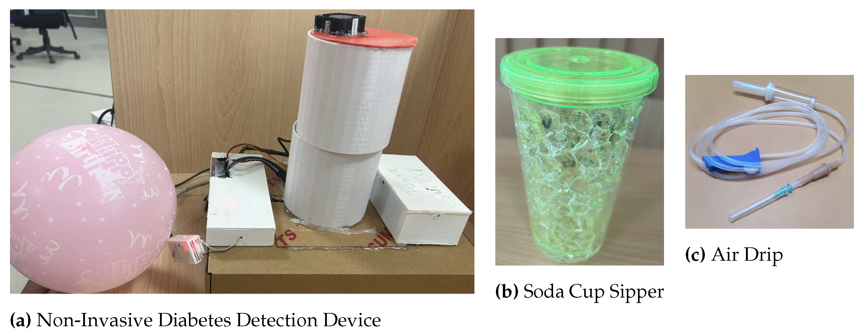
Figure 2.
Block Diagram of our Diabetes Detection system
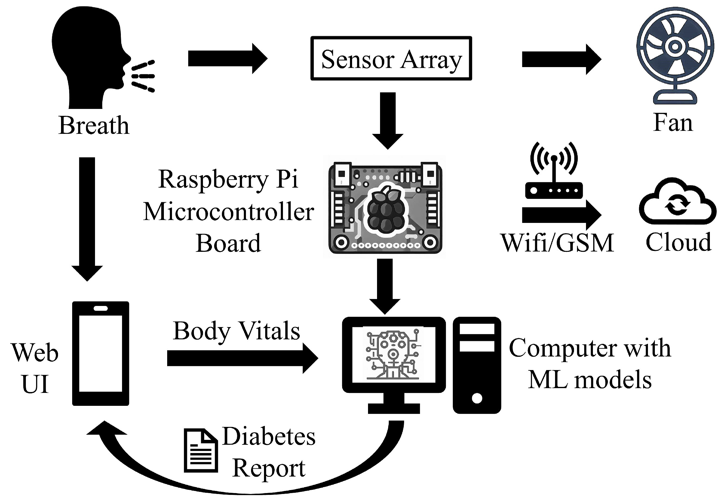
Figure 3.
Web Interface for entering details and sensor’s response to a breath sample.
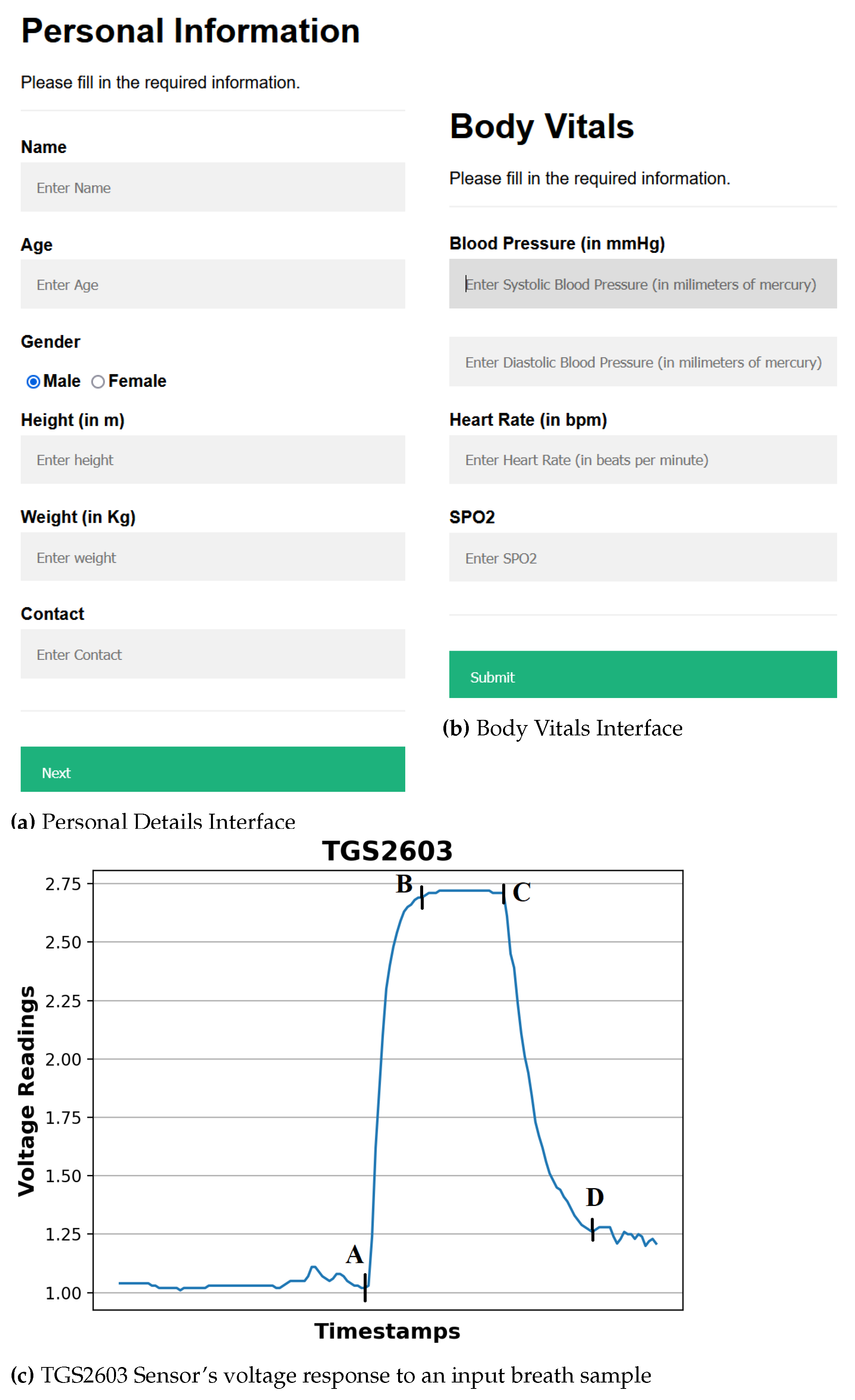
Figure 4.
Diabetes Report Viewing Web-Interface.
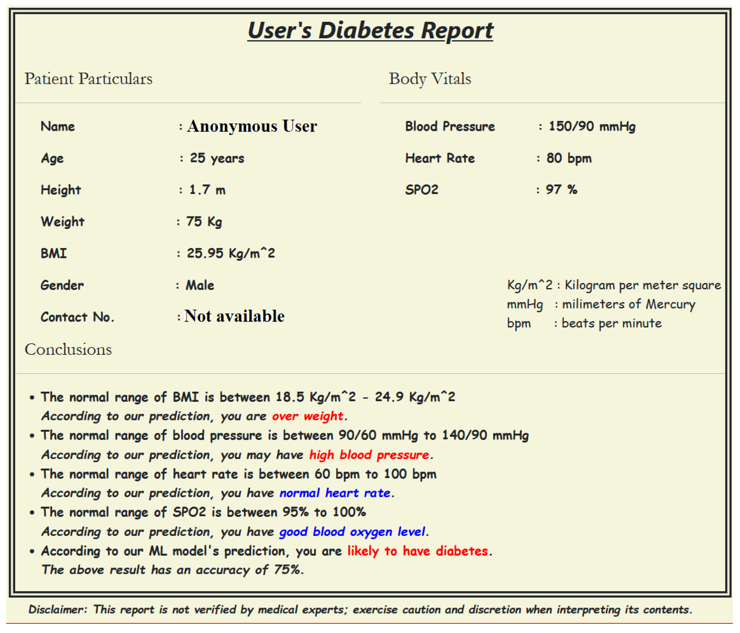
Figure 5.
SHAP Plot representing the impact of features on classification decision.
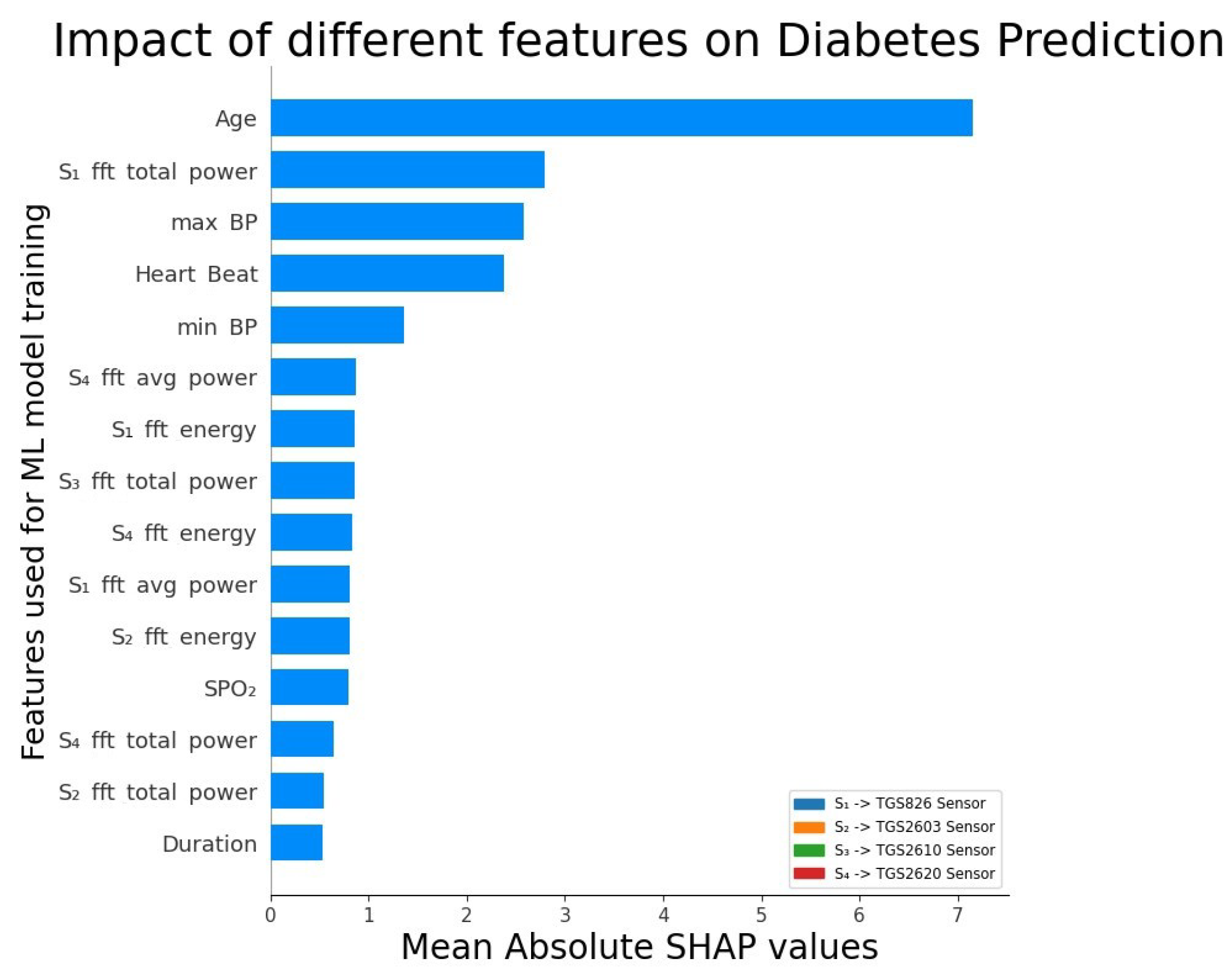

Table 1.
MOSFET-based Electrochemical Sensors used in the device.
| Sensor Model | Manufacturer | VOCs sensitivity | Sensitivity range (in ppm)1 |
|---|---|---|---|
| TGS826 | Figaro Inc., Osaka, Japan | VOCs, NH_3 | 30-5000 |
| TGS2610 | Figaro Inc., Osaka, Japan | H_2, VOCs | 500-10,000 |
| TGS822 | Figaro Inc., Osaka, Japan | VOCs, H_2, CO | 50-5000 |
| TGS2602 | Figaro Inc., Osaka, Japan | VOCs, NH_3, H_2S | 1-30 |
| TGS2600 | Figaro Inc., Osaka, Japan | H2, VOCS, CO | 1-100 |
| TGS2603 | Figaro Inc., Osaka, Japan | NH_3, H_2S | 1-10 |
| TGS2620 | Figaro Inc., Osaka, Japan | VOCs, H_2 | 50-5000 |
| MQ138 | Figaro Inc., Osaka, Japan | VOCs | 5 - 500 |
| DHT22 | Aosong Electronics Co., Ltd. | Humidity (H) and | H: 0 - 100 RH, |
| Temperature (T) | T: -40 - 80 Celsius |
1 ppm: parts per million.
Table 2.
List of features extracted from sensor voltage data.
| Base Feature | Feature used | Description |
|---|---|---|
| CurveMagnitude | abs(CurveMagnitude) [27] | The absolute value of curve magnitude values. |
| max(CurveMagnitude) [28] | The maximum of curve magnitude values. | |
| min(CurveMagnitude) [29] | The minimum of curve magnitude values. | |
| mean(CurveMagnitude) [30] | The mean or average of curve magnitude values. | |
| stdDev(CurveMagnitude) [31] | The median curve magnitude values. | |
| FirstDerivative [32] | max(FirstDerivative) | The maximum of first derivative of signal values. |
| min(FirstDerivative) | The minimum of first derivative of signal values. | |
| mean(FirstDerivative) | The mean of first derivative of signal values. | |
| abs(FirstDerivative) | The absolute value of the first derivative. | |
| stdDev(FirstDerivative) | The square root of the variance of the first derivative. | |
| SecondDerivative [32] | max(SecondDerivative) | The maximum of second derivative of signal values. |
| min(SecondDerivative) | The minimum of second derivative of signal values. | |
| mean(SecondDerivative) | The mean of second derivative of signal values. | |
| abs(SecondDerivative) | The absolute value of the second derivative. | |
| stdDev(SecondDerivative) | The square root of the variance of the second derivative. | |
| Slope and Integral | ||
| of five intervals [33] | Slope of five intervals | The slope of the five intervals of the curve1. |
| Integral of five intervals | The integral of the five intervals of the curve1. | |
| Phase |  |
It represents the integral of derivative over the magnitude values [34]. |
| Fast Fourier | phase | The phase is calculated based on the fft of the sensors’ reponse. |
| Transform | powerSpectrum | The square of the absolute value of fft transform. |
| (fft) [35,36] | spectralEntropy | It represents the entropy of power spectrum. |
| Wavelet [37] | waveletCoeffs | Coefficients of wavelet transformation of the sensor’s response signal. |
| Peak [38] | height | The height of the peak. |
| width | The width of the peak. | |
| area | The trapezoidal area of the peak. | |
| Shape | skewness [39] | The measure of the asymmetry of a distribution, where a positive skew indicates a longer tail on the right side and a negative skew indicates a longer tail on the left side. |
| kurtosis [40] | The measure of the tailedness of a distribution; a positive value indicates fatter tails and a negative value indicates thinner tails. | |
| entropy [41] | The measure of the disorder or randomness of a shape; a higher entropy indicates a more disordered or random shape. | |
| Auto-Regressive (AR) [42] | coefficients | These represent the relationships between past and current values of the model. |
| predictionError | The difference between the actual observed value and the ar-model’s predicted value. | |
| Short-time Fourier transform (STFT) [43] |
dominantFrequency | The frequency component that has the highest magnitude of the signal. |
| avg(magnitude(STFTcoeffs)) | The average magnitude of the STFT coefficients, calculated by taking the mean of the magnitudes over all the time frames. | |
| Sum(magnitude(STFTcoeffs)) | The sum of the magnitudes of all the STFT coefficients. | |
| energy(STFT) | The overall power of the signal in the frequency domain. | |
| centroid(STFTcoeffs) | The weighted average of the frequencies in the STFT, where the weights are the magnitudes of the STFT coefficients. | |
| bandwidth(STFT) | The range of frequencies represented by a single STFT coefficient, determined by the window length. | |
| rolloff(STFT) | The frequency at which the magnitude of the STFT coefficients drops to -3dB, typically used as a measure of the sharpness of the transition between the passband and the stopband. |
1 Five equal distance intervals are created from the sensor’s response voltages for a breath sample.
Table 3.
Parameter combination of different ML. techniques used for diabetes prediction.
| ML Classifiers | Parameter name | Parameter values |
|---|---|---|
| Decision Tree | criterion | (`gini’, `entropy’, `log_loss’) |
| splitter | (`best’, `random’) | |
| max depth | (2 to 10, step size of 1) | |
| min samples split | (2 to 10, step size of 1) | |
| Support Vector | C | (0.1 to 10, step size of 0.1) |
| kernel | (`linear’, `poly’, `rbf’, `sigmoid’, `precomputed’) | |
| degree | (3 to 10, step size of 1) | |
| gamma | (`scale’, `auto’, , `float’) with (0.001 to 1, step size of 0.005) for `float’ | |
| GradientBoost | learning rate | (0.01 to 10, step size of 0.01) |
| n estimators | (5 to 500, step size of 5) | |
| subsample | (0.01 to 1, step size of 0.01) | |
| criterion | (`friedman mse’, `squared error’) | |
| min samples split | (2 to 10, step size of 1) | |
| max depth | (2 to 10, step size of 1) | |
| RandomForest | n estimators | (5 to 500, step size of 5) |
| criterion | (`gini’, `entropy’, `log loss’) | |
| min samples split | (2 to 10, step size of 1) | |
| max depth | (2 to 10, step size of 1) | |
| max features | (`sqrt’, `log2’) | |
| min samples leaf | (1 to 10, step size of 1) | |
| KNeighbors | n neighbors | (5 to 100, step size of 5) |
| weights | (`uniform’, `distance’) | |
| algorithm | (`auto’, `ball tree’, `kd tree’, `brute’) | |
| leaf size | (30 to 100, step size of 3) | |
| ElasticNet | alpha | (0.01 to 1, step size of 0.01) |
| l1 ratio | (0.01 to 1, step size of 0.01) | |
| fit intercept | (True, False) | |
| max iter | (1000 to 5000, step size of 100) | |
| selection | (`cyclic’, `random’) | |
| Ridge | solver | (`auto’, `svd’, `cholesky’, `lsqr’, `sparse_cg’, `sag’) |
| fit intercept | (True, False) | |
| max iter | (1000 to 5000, step size of 100) | |
| Lasso | alpha | (0.1 to 10, step size of 0.1) |
| fit intercept | (True, False) | |
| copy X | (True, False) | |
| max iter | (1000 to 5000, step size of 100) | |
| selection | (`cyclic’, `random’) | |
| LogisticRegression | penalty | (`l1’, `l2’, `elasticnet’, None) |
| dual | (True, False) | |
| C | (0.1 to 10, step size of 0.1) | |
| fit intercept | (True, False) | |
| solver | (`lbfgs’, `liblinear’, `newton-cg’, `newton-cholesky’, `saga’, `sag’) | |
| max iter | (1000 to 5000, step size of 100) | |
| multi class | (`auto’, `ovr’, `multinomial’) | |
| XGBoost | max depth | (1 to 10, step size of 1) |
| alpha | (0.1 to 10, step size of 0.1) | |
| booster | (`gbtree’, `gblinear’) | |
| eta | (0.01 to 1, step size of 0.01) | |
| min child weight | (1 to 10, step size of 1) |
Table 4.
Performance Comparison using Five-fold Cross-validation, ADASYN and SMOTE balancing, and 80:20 split for training and testing with Hypertuned ML models.
Table 4.
Performance Comparison using Five-fold Cross-validation, ADASYN and SMOTE balancing, and 80:20 split for training and testing with Hypertuned ML models.
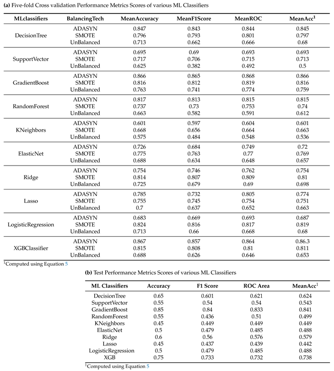
Table 5.
Features used for Experiments (subset of features described in Table 2).
Table 5.
Features used for Experiments (subset of features described in Table 2).
| Feature | Description |
|---|---|
| Age | age of the user. |
| Gender | gender of the user, i.e., male, female, or other. |
| BP | User’s max and min BP values |
| SPO2 | Oxygen level in Blood |
| Heart Rate | Heart Rate of the Patient. |
| Fast Fourier Transform (fft) |
phase powerSpectrum spectralEntropy |
| Phase |  |
| FirstDerivative | max(FirstDerivative) |
| min(FirstDerivative) | |
| mean(FirstDerivative) | |
| abs(FirstDerivative) | |
| stdDev(FirstDerivative) | |
| SecondDerivative | max(SecondDerivative) |
| min(SecondDerivative) | |
| mean(SecondDerivative) | |
| abs(SecondDerivative) | |
| stdDev(SecondDerivative) | |
| Slope and Integral | Slope of five intervals1. |
| of five intervals | Integral of five intervals1. |
1 Five equal distance intervals are created from the sensor’s response voltages for a breath sample.
Table 6.
Best hyper tuned parameter values for the ML techniques.
| ML Classifiers | Hyper tuned Parameter values |
|---|---|
| DecisionTree | criterion: `entropy’, splitter: `best’, max depth: 5, min samples split: 2 |
| SupportVector | C: 10, kernel: `rbf’, degree: not relevant1, gamma: `auto’ |
| GradientBoost | learning rate: 1, n estimators: 100, subsample: 1, criterion: `friedman mse’, min samples split: 2, max depth: 3 |
| RandomForest | n estimators: 100, criterion: `entropy’, min samples split: 2, max depth: 9, max features: `sqrt’, min samples leaf: 1 |
| KNeighbors | n neighbors: 7, weights: `distance’, algorithm: `auto’, leaf size: 30 |
| ElasticNet | alpha: 0.1, l1 ratio: 0.5, fit intercept: `True’, max iter: 1000, selection: `cyclic’ |
| Ridge | solver: `auto’, fit intercept: `True’, max iter: 1000 |
| Lasso | alpha: 0.1, fit intercept: `True’, copy X: `True’, max iter: 1000, selection: `cyclic’ |
| LogisticRegression | penalty: `l2’, dual: `False’, C: 10, fit intercept: `True’, solver: `lbfgs’, max iter: 1000, multi class: `ovr’ |
| XGBoost | max depth: 5, alpha: 0.1, booster: `gbtree’, eta: 0.3, min child weight: 1 |
1only relevany for poly or sigmoid kernel.
Disclaimer/Publisher’s Note: The statements, opinions and data contained in all publications are solely those of the individual author(s) and contributor(s) and not of MDPI and/or the editor(s). MDPI and/or the editor(s) disclaim responsibility for any injury to people or property resulting from any ideas, methods, instructions or products referred to in the content. |
© 2023 by the authors. Licensee MDPI, Basel, Switzerland. This article is an open access article distributed under the terms and conditions of the Creative Commons Attribution (CC BY) license (http://creativecommons.org/licenses/by/4.0/).
Copyright: This open access article is published under a Creative Commons CC BY 4.0 license, which permit the free download, distribution, and reuse, provided that the author and preprint are cited in any reuse.


