A Statistical and Machine Learning–Driven Framework for Predictive and Explainable Classification of Non-Invasive Blood Glucose Levels Using Photoplethysmography

1. Introduction

Diabetes mellitus is a long-term metabolic disorder characterized by recurring hyperglycemia and is the largest global health problem. In 2021, the International Diabetes Federation (IDF) had estimated that about 537 million adults worldwide had diabetes and increased to 643 million in 2030, which validates the importance of effective surveillance activities [1]. There are three types of measuring blood glucose, i.e., invasive, minimal invasive, and non-invasive. In invasive techniques, the two commonly applied methods are HbA1c measurement, traditional self-testing measurement, and continuous glucose monitoring (CGM). The fasting plasma glucose (FPG) test (oral glucose) [2,3] has formed the basis for conventional diagnostic techniques for the diagnosis of diabetes based on the measurement of HbA1c. HbA1c measurement necessitates fasting as well as several visits and blood sampling, which, being uncomfortable and intrusive, may be avoided by patients. Traditional self-testing of blood glucose via finger-prick testing is still invasive and laborious, which is associated with poor compliance and inadequate glycemic control [4]. CGM is considered one of the most accurate glucose measurement techniques that overcome the weaknesses of both HbA1c and the finger-prick method. However, all three invasive measurement techniques do not detect early-stage diabetes outcomes in deferred treatment [5]. The minimal invasive also requires similar blood sample collection, which is expensive and not practical for the majority of patients on a sustained basis [6]. To counter these limitations, non-invasive blood glucose monitoring (NIBGM) techniques were sought out as a feasible alternative as they measure using optical instruments without the need for blood sample collection or finger pricking. Of these, optical techniques, particularly photoplethysmography (PPG), have been of particular interest owing to their cost-effectiveness, simplicity of use, and wearability [7,8]. PPG measures volumetric changes of blood in microvascular tissues and offers a substantial volume of temporal and frequency-domain data that is quite pertinent to changes. However, the comparative accuracy of measuring blood glucose using non-invasive methods is still not matchable to invasive measuring techniques. Therefore, there is a need to explore new ways to increase the effectiveness of non-invasive types of measurements for accurate detection. This research employed both types of measuring methods for the collection of patient data.

The use of artificial intelligence (AI) in the field of diabetes has been presented as a solution for predicting early cure based on the data obtained from invasive, minimal invasive, and non-invasive techniques. A major development is detecting type 2 diabetes via voice analysis coupled with AI. Six Klick Labs studies revealed that when six AI algorithms are used to analyze ten-second vocal recordings, they may precisely identify type 2 diabetes with great sensitivity and specificity. This method, especially helpful in resource-constrained environments, offers a non-invasive, affordable, and quick screening solution [9]. For continuous glucose monitoring, wearable devices using optical and microwave-based sensing techniques are also being developed. Real-time glucose information from these sensors ideally helps to better manage diabetes and hence reduces disease-related consequences [10]. Reviews of novel non-invasive technologies further emphasize the role of such devices in the future of diabetes care [11]. Therefore, although non-invasive approaches seem promising, extensive verification and legal consent are necessary steps toward their general usage [12].

Wearable, Internet of Things (IoT)-enabled photoplethysmogram (PPG) sensors are becoming increasingly important in enabling real-time, remote, and personal glucose monitoring services [3]. Explainable Artificial Intelligence (XAI) methods such as SHAP have promoted model transparency and trust, making ML-based systems interpretable at a clinical level [13]. These developments point toward economical, non-invasive, and accurate glucose monitoring devices. By focusing on optical signal analysis, efficient ML algorithms, and edge-device integration, future systems will be able to provide patient-centric, accurate monitoring at scale. This work pushes these developments one step ahead, with optimized signal processing and AI strategies for efficient invasive and NIBGM up to 84–89% accuracy to bridge the research-to-clinic gap.

2. Literature Review

The literature represents machine learning (ML), neural networks (NN), deep learning (DL), and their ensembles for the assessment and prediction of accurate detection of blood glucose. Machine learning is the earliest and most extensively used technique to identify blood glucose. For example, research on smartphone- and video-based PPG has shown that glucose levels can be estimated using several statistical and machine learning techniques including PCR, Random Forest, SVR, and PLS [2]. In clinical pilot tests, prototypes for in-ear and wrist PPG have been evaluated to show great accuracy in Clarke/Parkes error grids, particularly when partnered with meticulous preprocessing and machine learning modeling [14,15]. The importance of signal processing and feature engineering highlights the methods like denoising, segmentation, empirical mode decomposition, spectral entropy, and derivative features [16,17,18]. The use of tree-ensemble methods such as CatBoost, XGBoost, Random Forest (RF), and LightGBM has shown promise or explored potential in non-invasive blood glucose prediction by achieving mean absolute error (MAE) between 8 and 15 mg/dL [13,19]. Due to considerably better classification and regression performance, hierarchical feature fusion (e.g., multi-view attention + cascaded BiLSTM) outperforms standard methods [20].

Neural network approaches have also been applied. For example, 84–90% predictive performance concerning blood glucose levels and classification of diabetes status was reported using Random Forest, SVMs, and neural networks [21]. Prominent NIR spectroscopic systems, such as the iGLU family devices, have demonstrated excellent performance using polynomial regression and deep neural network (DNN) models with strong accuracy in bench and small-scale trials [22,23]. Classification problems such as differentiating diabetes from non-diabetes or assessing risk levels usually have better nominal accuracy than regression. Ensemble classifiers, SVMs, and CNNs have shown impressive classification accuracies ranging from 84% to 98% across different datasets [24,25]. Recent work on multi-wavelength PPG demonstrated that incorporating near-infrared and environmental parameters improves estimation accuracy [26].

Hybrid DL architectures such as CNN-GRU further decreased MAE to 3 mg/dL. The selection of features is a primary part of studies related to diabetic datasets. Usually, feature selection consists of non-statistical or statistical methods. To lower feature dimensionality, a hybrid pipeline using recursive feature elimination (RFE) with isolation forest improved classification performance [27]. Authors have used several ML models evaluated to detect high blood glucose by performing thorough feature engineering on wrist PPG signals and combining those with demographic data via 10-fold cross-validation. Stringent feature engineering on wrist PPG signals, coupled with demographic data and tested on various ML models through 10-fold cross-validation, has also yielded good results [18]. Recent research highlights the importance of feature selection methods including random forest importance, ridge regression, LASSO, recursive feature elimination (RFE), ANOVA, and chi-square [28,29], showing feature-selection techniques (filter methods, wrapper via RFE, and embedded techniques like LASSO) across several diabetes datasets.

Finally, Parvez and Mufti [30] emphasized that statistical validation is essential in hybrid machine learning models and demonstrated calibration measures including Brier score, calibration slope, and intercept, together with reliability (calibration) plots to visually evaluate model calibration. To measure uncertainty in calibration estimates, they also determined 95% confidence intervals using bootstrap sampling (1,000 resamples). In another study, Casacchia et al. [31] used electronic health record (EHR) data to construct a prediction model for elevated HbA1c risk (a diabetes biomarker) and assessed calibration with calibration curves and summary metrics including the Brier score. Hageh et al. [32] in research on improving type 2 diabetes (T2D) prediction explicitly referenced calibration curves and Brier scores for probability reliability assessment in their evaluation framework. Kornas et al. [33] conducted external validation of a diabetes prediction model and noted the general Brier score as an indicator of prediction error in a real-world population, while Templeman et al. [34] and others provided similar validation in BMJ Evidence-Based Medicine. Such examples show that DL-based methods are sometimes associated with poorer calibration compared to Cox models, showing a lower Brier score [35]. A meta-review of ML models predicting diabetic complications noted that few studies reported calibration using Brier score, Hosmer–Lemeshow test, or Greenwood–D’Agostino–Nam test, and recommended internal validation with calibration curves [36]. Therefore, it is concluded that the statistical interpretation establishes the dependability of the datasets, features, and applied ML, NN, and DL models.

3. Methodology

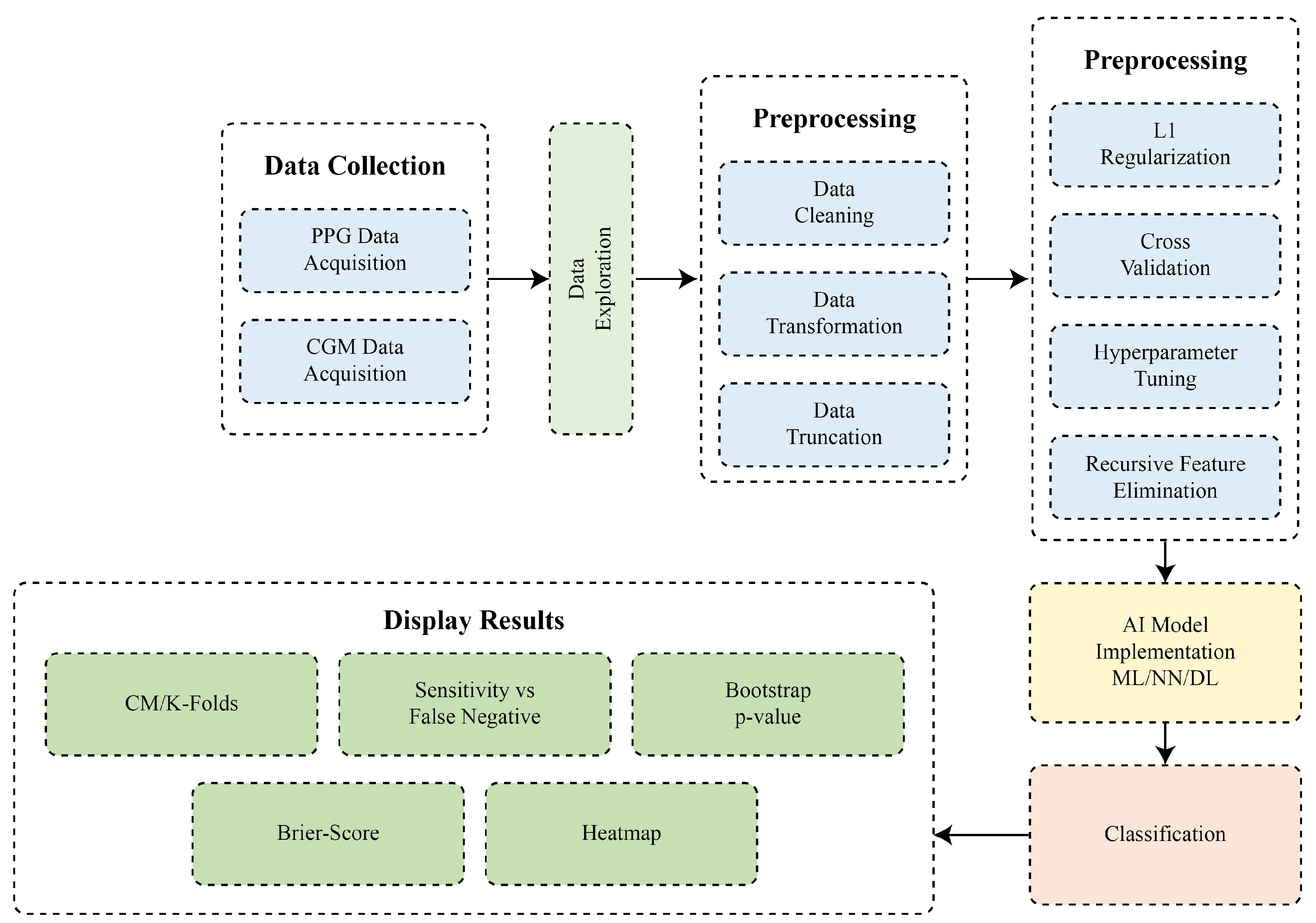
In this study, we present the analytical framework illustrated in Figure 1. The process begins with data acquisition from Continuous Glucose Monitoring (CGM) devices and photoplethysmography (PPG) signals. Then, the dataset is subjected to preprocessing ensuring accuracy, consistency, and readiness for analysis. From the refined signals, a large number of statistical, morphological, time-domain, and frequency-domain feature extractions are made. Then, the feature selection and data-class-balanced for training are performed toward the end of the training process before entering the model. The final stage of model output is that machine learning classifiers have been implemented, with a special mention of the ensemble algorithms and neural networks, and these results would then go through an established performance assessment metric. Detailed descriptions of individual methodology components are provided in the following subsections.

Figure 1. Research methodology for non-invasive glucose monitoring.

Figure 1. Research methodology for non-invasive glucose monitoring.

3.1. Dataset

BIG IDEAs Lab Glycemic Variability and Wearable Device Data (Peter Cho, n.d.) available to the public, was employed to assess the practicability of wearable sensing for the early identification of glycemic dysregulation. Sixteen subjects (35–65 years, HbA1c: 5.2–6.4%) wore a Dexcom G6 continuous glucose monitor (CGM) and an Empatica E4 wristband during 8–10 days with standardized meals given every other day. The CGM measured interstitial glucose every five minutes, whereas the E4 obtained multimodal physiological signals, such as photoplethysmography (PPG, 64 Hz), electrodermal activity (EDA), skin temperature, and accelerometery. While the cohort size is small, the signal-level dataset is sizable. Every raw PPG trace comprises more than 50 million samples, generating hundreds of millions of data points for the study. These signals were then converted to structured datasets after synchronization, normalization, and preprocessing, providing about 14,000 balanced instances per class. High temporal resolution and multimodal integration supply adequate data diversity for firm feature extraction, machine learning model training, and proof-of-concept verification in non-invasive glucose prediction.

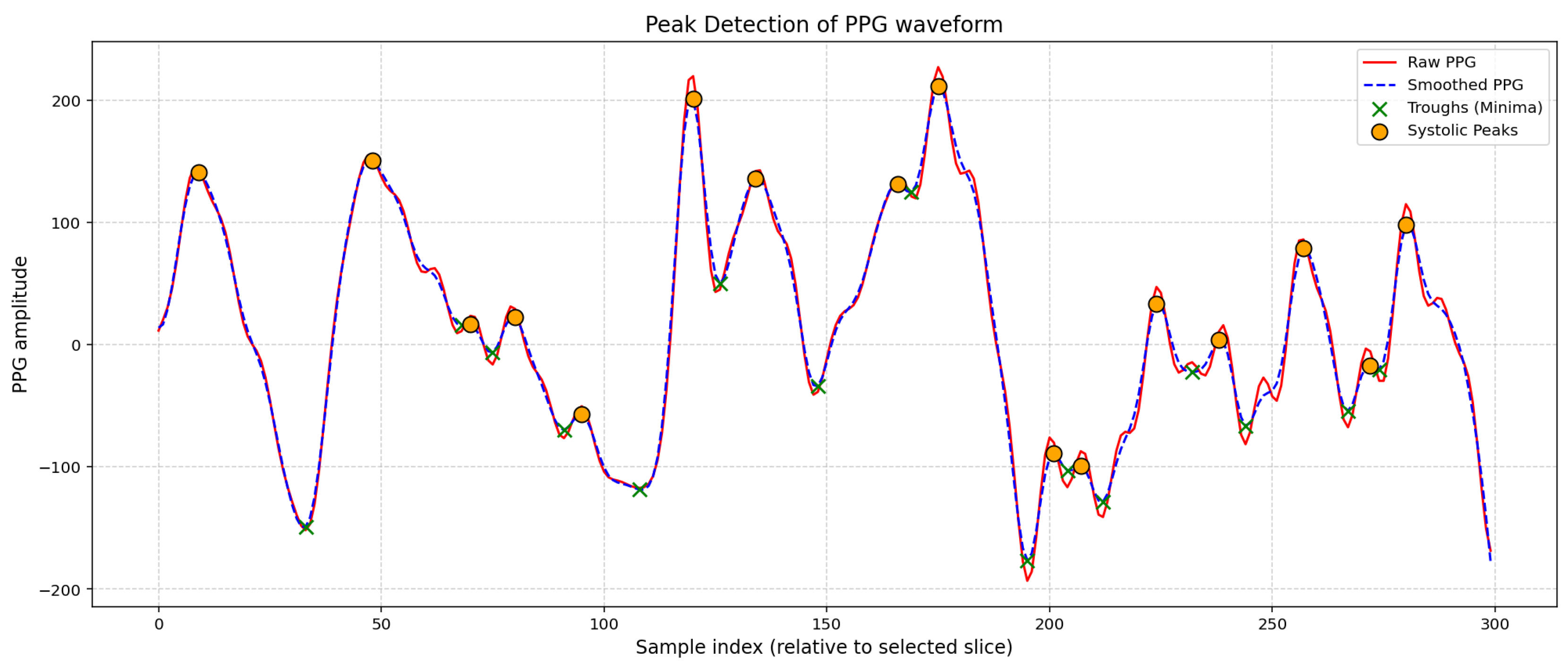
Figure 2. Peak detection of PPG raw waveform.

Figure 2. Peak detection of PPG raw waveform.

3.2. Preprocessing

The dataset included raw photoplethysmography (PPG) signals and continuous glucose monitor (CGM) data for 16 participants over 8-10 days. Each CGM measurement was taken every 5 minutes while PPG was sampled at a faster rate. For consistency, temporal equalization was performed by segmenting PPG signals into 5-minute periods that matched with respective CGM measurements to allow for reliable labeling of segments to hypoglycemic, normoglycemic, prediabetic, and hyperglycemic bins. Data cleaning consisted of discarding signal segments where there was no longer continuous signal and removing entries with missing values. There was no dedicated filtering or removal of motion artifacts in the data; while it was not the purpose, the segments taken as the time-aligned windows were of high quality. In order to mitigate differences of scale between features min-max normalization was used. In addition, the inherent class imbalance was addressed with the Synthetic Minority Oversampling Technique (SMOTE) to create additional synthetic samples of minority classes to create a more balanced dataset for training.

3.3. Feature Selection and classification

3.3.1. Feature Extraction and Selection

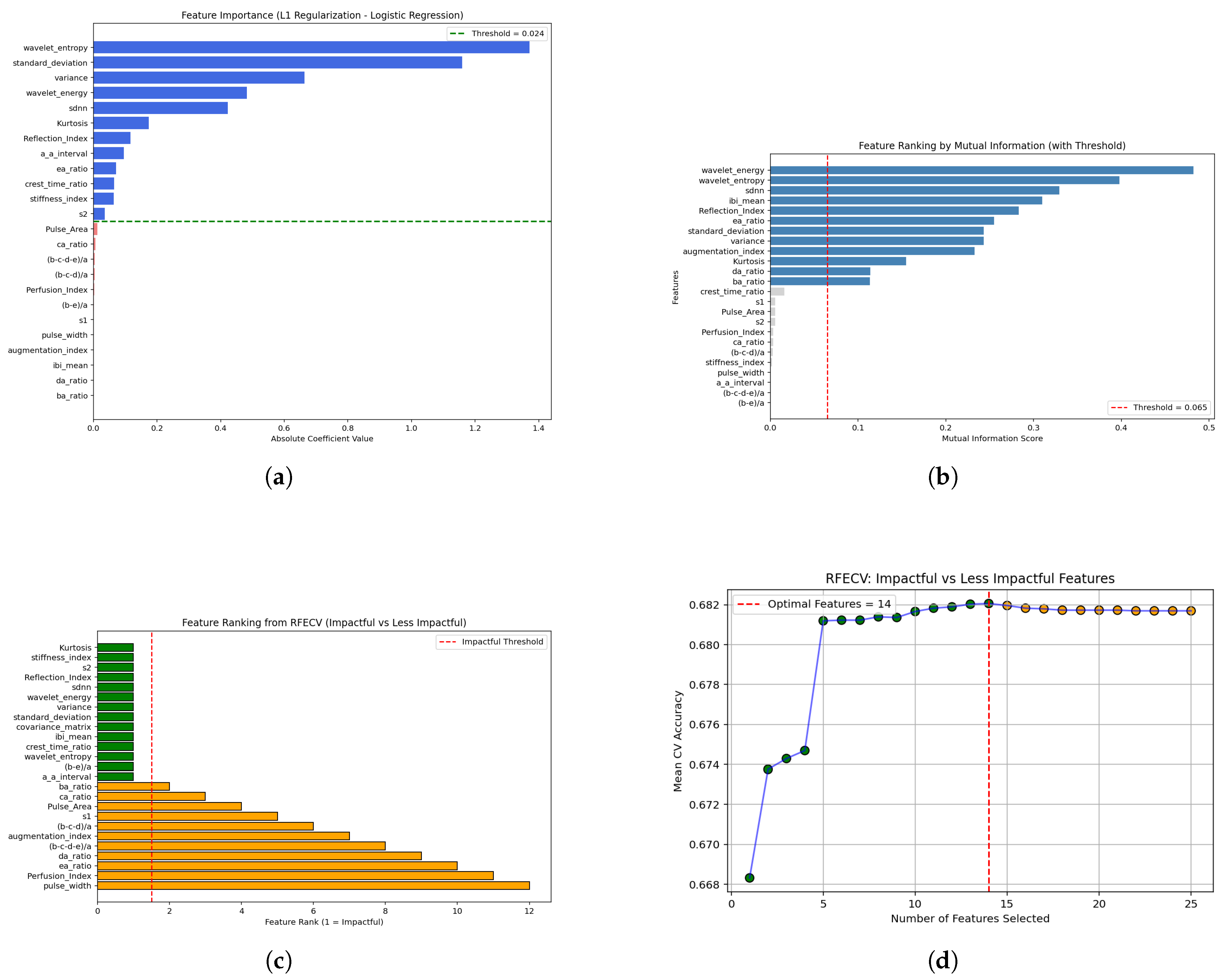
From every pre-processed PPG segment, we derived 24 physiologically relevant features initially based on three classes of features—morphological (e.g. reflection index, stiffness index, crest-time ratio, A-A interval, amplitude ratios), statistical (standard deviation, variance, kurtosis) and time-domain (SDNN, mean IBI, S1 & S2 amplitudes) as well as frequency-domain (wavelet energy, wavelet entropy). Then a rigorous feature selection pipeline was applied straight to the dataset to extract the most discriminative predictors, which consisted of L1-regularization (Lasso) coefficients, recursive feature elimination, cross-validation, and hyperparameter tuning simultaneously in one framework. With this approach, redundancy was eliminated, bias was reduced, and reproducibility was enhanced across validation folds. Ultimately, this method reliably converged on 12 impactful features: Kurtosis, Reflection Index, S2 amplitude, SDNN, Standard Deviation, Stiffness Index, Variance, Wavelet Energy, Wavelet Entropy, Crest-Time Ratio, A-A Interval, and EA Ratio, which showed both the most powerful and stable discriminative power for glycemic state classification. These 12 features are what formed the basis of input data for the machine learning models.

Figure 3. Comparative view of feature selection techniques: (a) L1-regularization for sparsity-based feature reduction; (b) hyperparameter tuning for best model configuration; (c) cross-validation for strong performance estimation and (d) for methodical feature ranking, recursive feature elimination (RFE).

Figure 3. Comparative view of feature selection techniques: (a) L1-regularization for sparsity-based feature reduction; (b) hyperparameter tuning for best model configuration; (c) cross-validation for strong performance estimation and (d) for methodical feature ranking, recursive feature elimination (RFE).

3.3.2. Classification

Within this research project, a four-class classification problem was defined to classify glucose levels into four states: hypoglycemic, normal, pre-diabetic, and hyperglycemic. This multi-class framework captures clinically meaningful classifications and allows us to investigate detailed patterns. To execute this task, six representative models were carefully selected from machine learning (ML), deep learning (DL), and neural network (NN) frameworks. From the ML approaches, LightGBM, Random Forest and CatBoost were selected for their high performance with structured features that represent complex relationships and imbalanced classes. From the DL family, we implemented a Convolutional Neural Network (CNN) to model local signal morphology from PPG waveforms using a hybrid BiLSTM + LightGBM ensemble, to learn sequentially and enhanced predictive performance via a gradient-boosted decision tree on the feature-level.

The chosen models provided a balanced comparison, enabling us to explore both stand-alone models as well as hybrid models under the same preprocessing conditions (timestamp equalization with CGM data, SMOTE balancing and a systematic feature selection using L1-regularization, recursive elimination, cross-validation and hyperparameter tuning). By evaluating multiple architectures on the same data, we aim to demonstrate not only the separate predictive power of each learner but a practical benefit of employing deep and ensemble approaches for FX continuous non-invasive glucose monitoring.

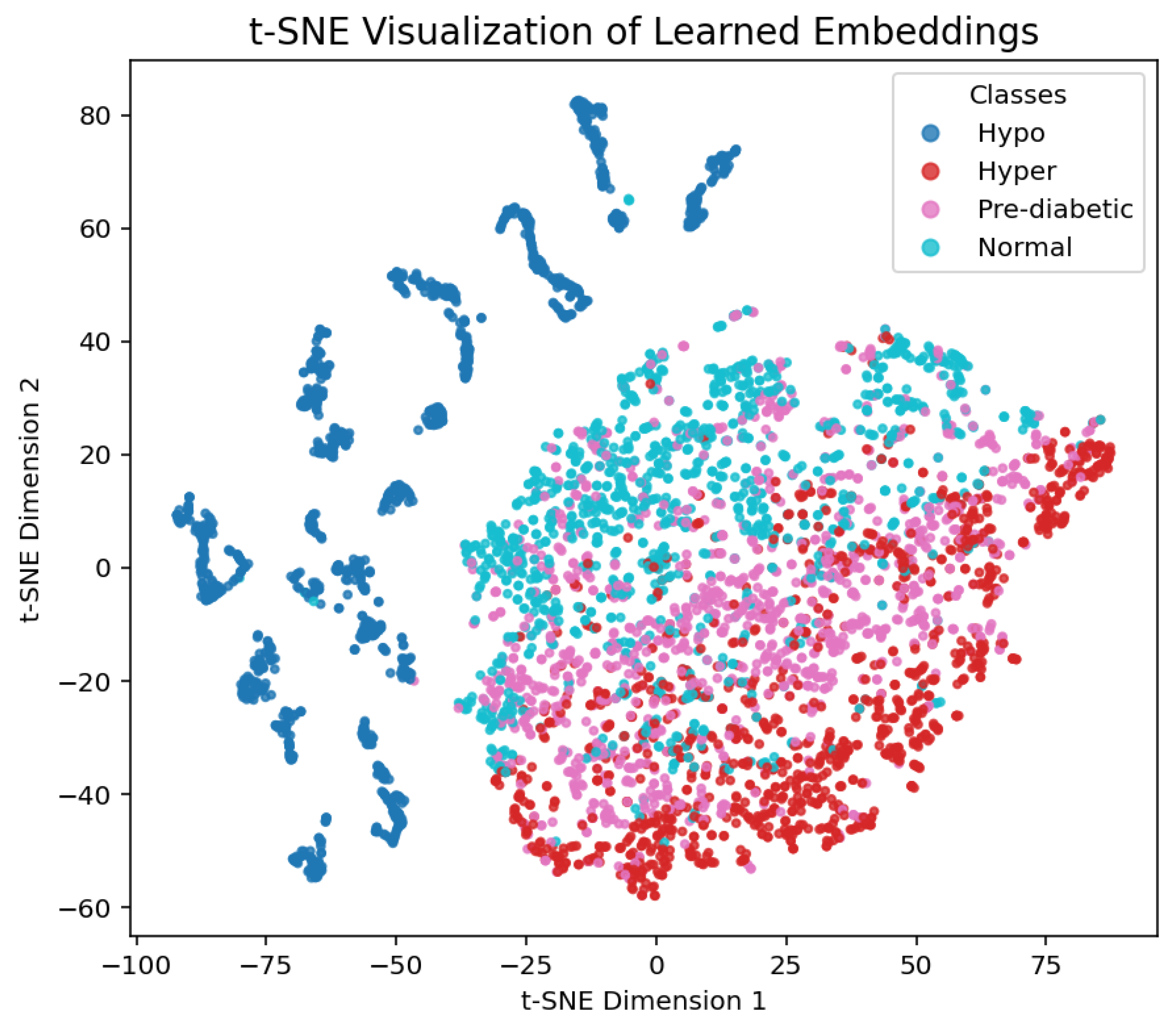
"While explicit motion artifact removal was not performed, the t-SNE visualization of the learned embeddings (Figure 4) suggests that the samples for different classes (hypo, hyper, pre-diabetic, normal). This suggests that the suggested dataset helps models learn strong representations and identify discriminative features, which in turn improves correct categorization of the several glycemic states.."

Figure 4. T-SNE visualization of learned embeddings.

Figure 4. T-SNE visualization of learned embeddings.

Light Gradient Boosting Machine (LightGBM):

LightGBM is a fast gradient boosting framework that employs a leaf-wise growth strategy, restricted to a maximum depth, in the learning process of decision trees. As a result, LightGBM offers lower memory and training duration for large datasets, while still attaining accuracy levels comparable or superior to traditional implementations. It is especially suited for physiological datasets with structured, high-dimensional feature sets with class imbalance, making it advantageous for non-invasive glucose prediction research.

Random Forest:

Random Forest is an ensemble learning technique that produces an array of decision trees with bootstrap samples of the model dataset, and with randomly generated subsets of model features. The model prediction is determined by aggregating the predicted responses from each individual tree, thus improving generalizability and preventing overfitting. As RF also has the ability to model non-linear interactions of model features, it is ideally suited for the classification of physiological signals.

CatBoost:

CatBoost is a gradient boosting algorithm developed to efficiently handle categorical features and reduce prediction shift. It makes use of ordered boosting as well as symmetric trees to reduce overfitting and increase stability of the model. CatBoost is effective at handling class imbalance, and in many instances, outperforms existing boosting methods in applied structured biomedical datasets.

Convolutional Neural Network (CNN):

Convolutional Neural Networks (CNN) are a deep learning approach that extracts hierarchy spatial features through several convolutive pooling layers. In this study, CNNs were employed to extract localized morphological changes of PPG waveform signals to discern patterns of raw physiological signals. CNNs are well-suited for class banking glucose categories, and data is discriminative by learning from signal segments.

Gradient Boosting (GB):

Gradient Boosting is a family of ensemble methods that build additive models in sequence - each weak learner (often a bootstrapped decision tree) is based on the resonances from previous learners. The predictably strong performance from the iterative optimization minimizes the loss function. GB methods work well on structured data, while also finite precise tuning may be necessary to avoid annealing.

BiLSTM + LightGBM Ensemble:

The proposed ensemble combines Bidirectional (BiLSTM) networks with LightGBM such that each level of prediction benefits from complementary strengths. The BiLSTM models can detect and analyze long-range temporal features in PPG signals, while LightGBM can parse distinctive features at the signal segment level. The BiLSTM layer predictions are passed to LightGBM for their high robustness and classification accuracy relative to either stand-alone model. The proposed hybrid model combines gradient-boosted decision trees with sequential learning to create a state-of-the-art approach to multi-class glucose classification. To avoid overfitting, a ten-fold cross-validation was performed to visualize the performance of the classifiers as mentioned above. The performance of the classifiers was measured using various performance metrics, including sensitivity, precision, F1-score, and classification accuracy, obtained from the confusion matrix. Table 1 describes the confusion matrix for a binary classification.

Table 1. Confusion matrix.

Description	Actual Positive	Actual Negative
Predictive Positive	True Positive (TP): The proportion of accurate forecasts in which the positive class is anticipated to be positive.	False Negative (FN): The quantity of inaccurate forecasts in which the positive class is anticipated to be negatively projected.
Predictive Negative	False Positive (FP): The quantity of erroneous forecasts in which the negative class is anticipated to be positive.	True Negative (TN): The quantity of accurately anticipated negative values for the negative class.

Table 1. Confusion matrix.

Description	Actual Positive	Actual Negative
Predictive Positive	True Positive (TP): The proportion of accurate forecasts in which the positive class is anticipated to be positive.	False Negative (FN): The quantity of inaccurate forecasts in which the positive class is anticipated to be negatively projected.
Predictive Negative	False Positive (FP): The quantity of erroneous forecasts in which the negative class is anticipated to be positive.	True Negative (TN): The quantity of accurately anticipated negative values for the negative class.

Accuracy: The percentage of correct predictions among all predictions, as shown in Equation (1).

$$\mathrm{Accuracy}={\displaystyle \frac{TP+TN}{TP+FP+FN+TN}}$$

(1)

Precision: The percentage of positive predictions that are actually true positives, defined in Equation (2).

$$\mathrm{Precision}={\displaystyle \frac{TP}{TP+FP}}$$

(2)

Recall: The proportion of actual positives that are correctly predicted as positive, as given in Equation (3).

$$\mathrm{Recall}={\displaystyle \frac{TP}{TP+FN}}$$

(3)

F1 Score: The harmonic mean of precision and recall, offering a balance between the two. Defined in Equation (4).

$$F{1}_{\mathrm{score}}={\displaystyle \frac{2\times \mathrm{Precision}\times \mathrm{Recall}}{\mathrm{Precision}+\mathrm{Recall}}}$$

(4)

4. Results and Discussion

The dataset used in this paper to extract results is an online available dataset named BIG IDEAs Lab Glycemic Variability and Wearable Device Data (Peter Cho, n.d.). The summary of results obtained for various classifiers is tabulated in Table 2. The detailed results of classifiers are presented in the subsequent sections.

Table 2. Summary of results of classifiers.

Classifier	Accuracy (%)
Ensemble	89
Light Gradient Boosting	89
Random Forest	88
CatBoost	84
Convolutional Neural Network	80
Gradient Boosting	79

Table 2. Summary of results of classifiers.

Classifier	Accuracy (%)
Ensemble	89
Light Gradient Boosting	89
Random Forest	88
CatBoost	84
Convolutional Neural Network	80
Gradient Boosting	79

4.1. Ensemble

Figure 5. 10-K-fold cross-validation confusion matrix illustrating classification outcomes for the ensemble model.

Figure 5. 10-K-fold cross-validation confusion matrix illustrating classification outcomes for the ensemble model.

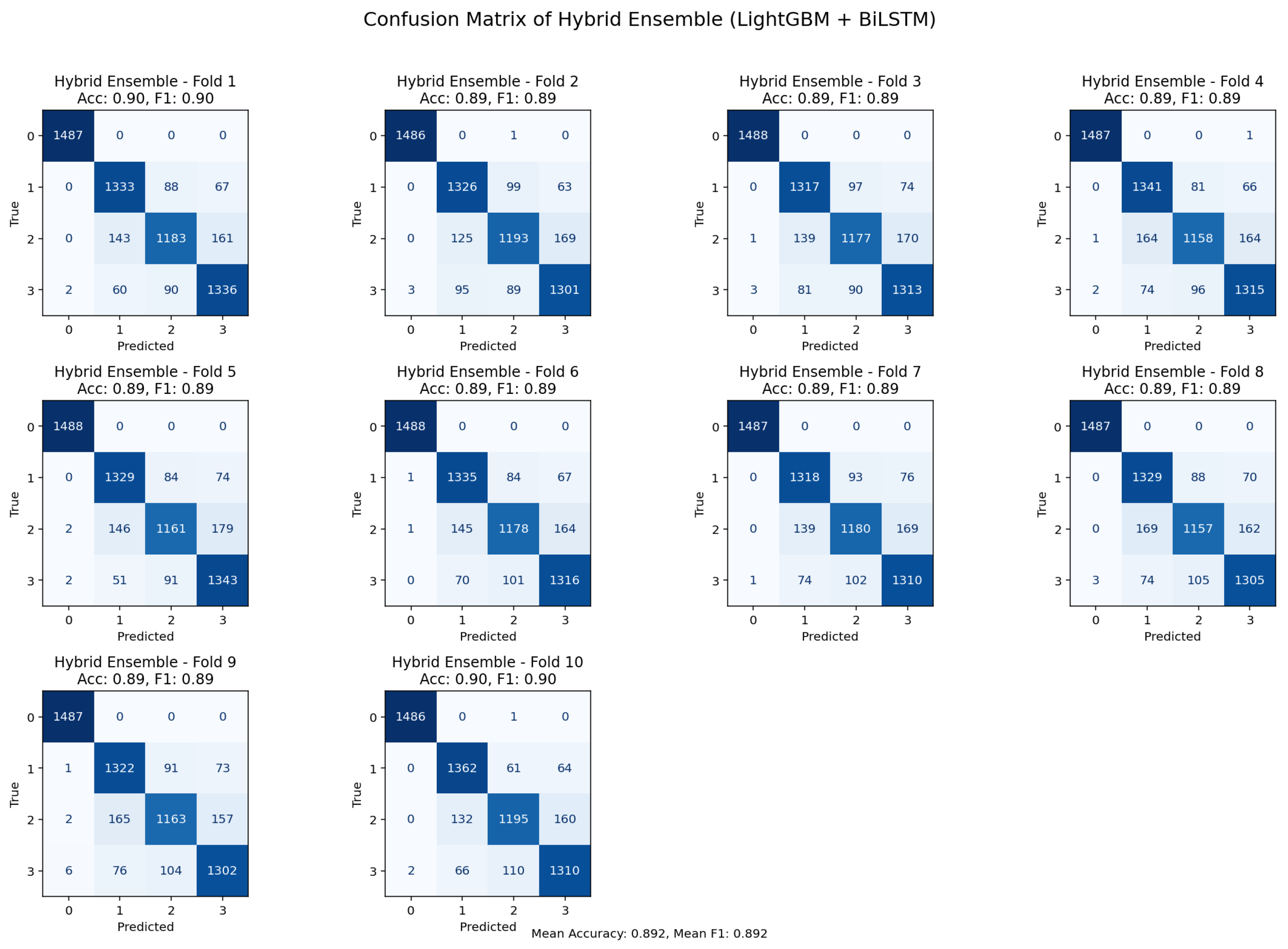
With accuracy and F1-scores for most folds, the bi-directional LSTM and LightGBM ensemble confusion matrices under 10-fold cross-validations showed fairly steady overall performance. returning values between 0.89 and 0.90. Most misclassification was seen in classes that were physiologically close, such as pre-diabetic physiological conditions and normal physiological ones, which have coinciding properties inside the PPG signal profile. These patterns imply that rather than ensemble model systematic bias, misclassification reflect actual underlying physiological resemblance. Collectively, the consistency across folds and the overall distribution of errors support the advantages of the ensemble method, and its robustness and clinical applicability.

Figure 6. Diagnostic plots for the ensemble model: (a) Calibration plot showing reliability of predictions; (b) Learning curve depicting convergence dynamics; (c) ROC and Precision–Recall curves illustrating class discrimination; and (d) Boxplot visualization of prediction outcome distribution.

Figure 6. Diagnostic plots for the ensemble model: (a) Calibration plot showing reliability of predictions; (b) Learning curve depicting convergence dynamics; (c) ROC and Precision–Recall curves illustrating class discrimination; and (d) Boxplot visualization of prediction outcome distribution.

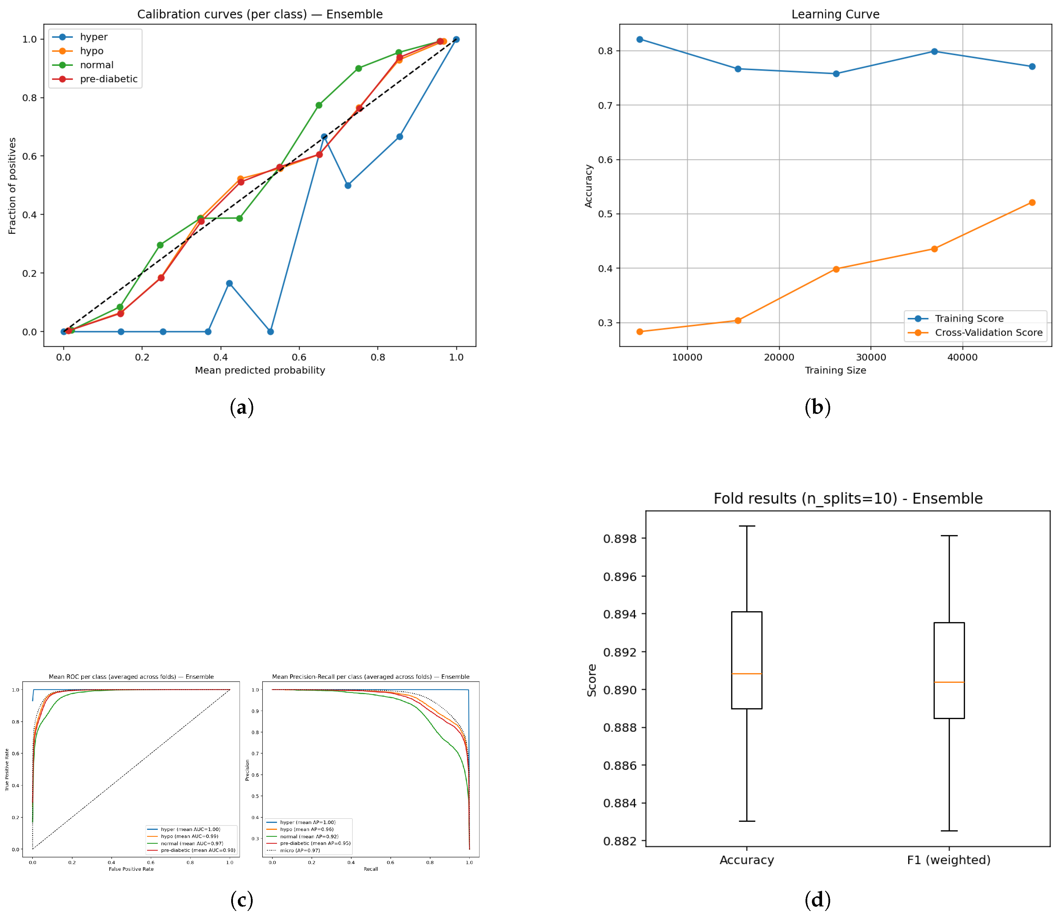
The assessment of the BiLSTM-LightGBM ensemble was conducted via calibration, learning, receiver operating characteristic (ROC), precision-recall and box plot analyses (Figure a–e). The calibration plots (Figure a) suggest that the predicted probabilities match closely to the observed probabilities across all classes indicating that the model outputs can be interpreted in clinical relevance and are reliable. The learning curve (Figure b) suggests that the training accuracy is stable and the validation performance is increasing confirming that the model is generalizing well and learning with still larger datasets. ROC curves (Figure c) consistently demonstrate high area under the curve (AUC) (0.97-1.00) indicating the four glucose states can be strongly separated, whilst precision-recall curves (Figure d) provide confidence in detecting the classification reliably, with mean average precision (AP) scores ranging from 0.92-1.00, indicating consistent detection across all glucose categories. Lastly, cross-validation box plots (Figure e) indicate narrow variability across accuracy and weighted F1 ( 0.89), providing confidence in the robustness and stability of the proposed ensemble specification across folds. Overall, these results confirm the model provided a well-calibrated, generalizable and reliable assessment for non-invasive diabetes monitoring.

Figure 7. Ensemble model analysis: (a) Bootstrap p-values indicating statistical reliability of ensemble estimates; (b) Sensitivity versus false negatives showing diagnostic robustness across classes.

Figure 7. Ensemble model analysis: (a) Bootstrap p-values indicating statistical reliability of ensemble estimates; (b) Sensitivity versus false negatives showing diagnostic robustness across classes.

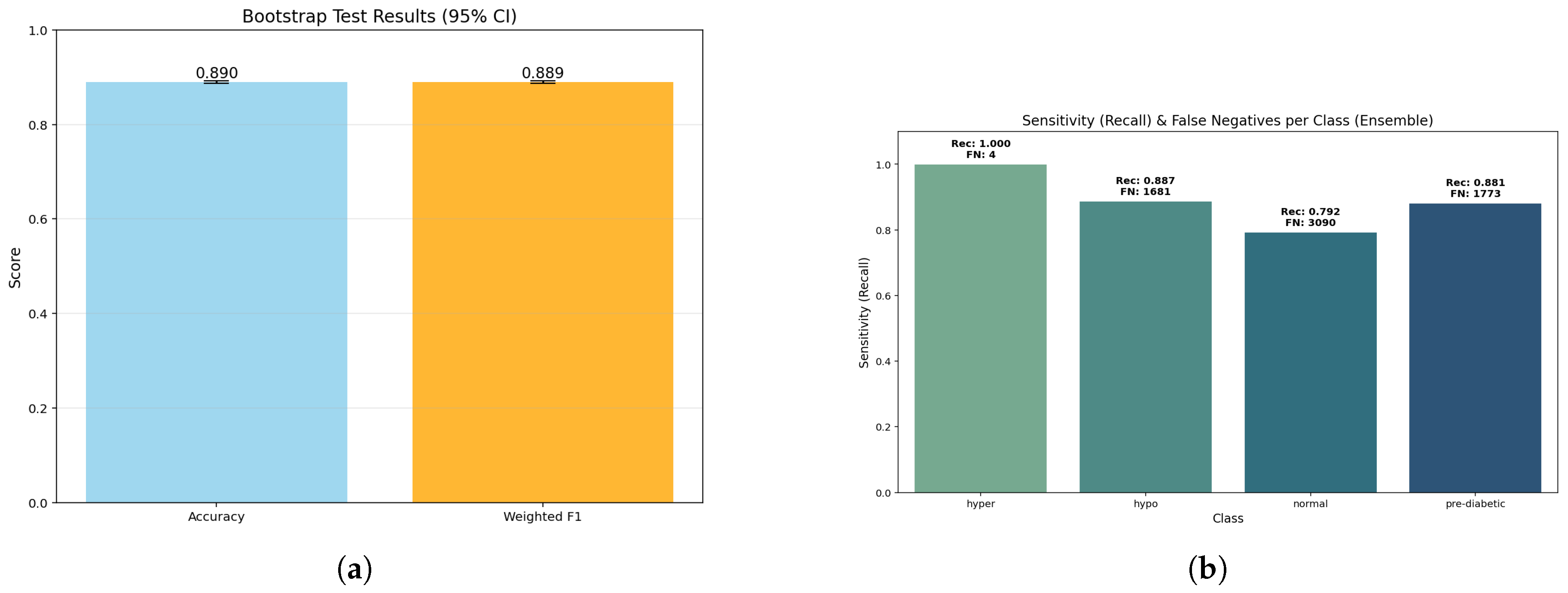
The bar plot shows essentially the same accuracy (0.890) and weighted F1 (0.889). The fact that these two values are so similar, confirmed with a bootstrap p-value of 1.0, indicates that the model holds balanced predictive capability across all classes without bias towards any particular class. Further, the bootstrap estimates were stable, thereby assuring that these estimates did not artificially inflate due to sampling variability.

The sensitivity bars indicate almost perfect detection of the hyperglycemia class (1.000, FN ≈ 4) while high recall is achieved for hypoglycemic (0.887, FN ≈ 1681) and pre-diabetic (0.881, FN ≈ 1773) classes. The lowest sensitivity is for the normal class (0.792, FN ≈ 3090); this suggests that some normal samples were classified into neighboring glucose states. Critically, this weighting shows the model’s clinical strength to avoid false negatives for high-risk categories (hyper and hypo) even if it achieves some loss of sensitivity in the normal range.

The ensemble model performed well, achieving an overall accuracy of 0.89 (95% confidence interval (CI); 0.887–0.892) and a weighted F1-score of 0.889, verifying that model performance remains reasonably level across all three categories. The macro recall was also 0.890, indicating that the model is behaving reasonably and not skewed towards any one single class, especially concerning inter-class dissociation. When it comes to calibration, the Brier scores were low, especially for the hyperglycemia class (0.00055) showing excellent calibration reliability for probability last risk situations. The Brier scores were slightly higher; 0.0611 for normal class and 0.0463 for pre-diabetic class, showing moderate uncertainty in borderline ranges, consistent with the expectations in clinical practice of inter-class overlaps. Overall, it is noteworthy to conclude that the ensemble method had overall strong performance and robustness aligned with clinical expectations, namely avoiding erroneous classifications for important clinical conditions.

4.2. LightGBM

Figure 8. Confusion matrix from 10-fold cross-validation highlighting predictive performance of the LightGBM model.

Figure 8. Confusion matrix from 10-fold cross-validation highlighting predictive performance of the LightGBM model.

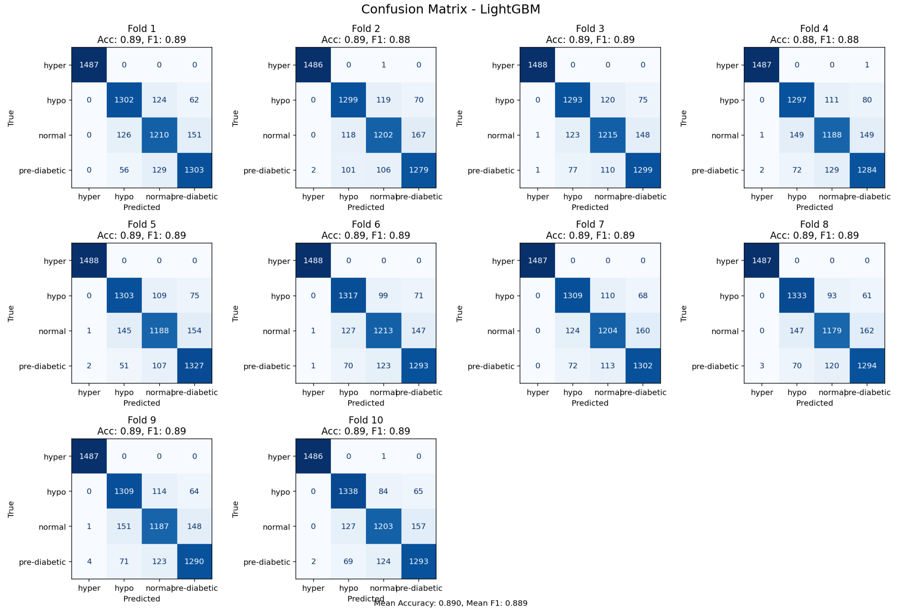
The LightGBM (gradient boosted tree) achieved an accuracy of 89% and performed consistently across all glycemic classifications. Misclassifications were primarily confined to transitional categories, which suggests the classifier was sufficiently sensitive to small physiological variations rather than bias. Overall, the gradient boosting mechanism served the purpose of adequately modeling complex non-linear interactions with the data.The LightGBM demonstrated excellent and consistent predictive performance, and was one of the most dependable classifiers in this research.

Figure 9. Diagnostic plots for the ensemble model: (a) Calibration plot showing reliability of predictions; (b) Learning curve depicting convergence dynamics; (c) ROC and Precision–Recall curves illustrating class discrimination; and (d) Boxplot visualization of prediction outcome distribution.

Figure 9. Diagnostic plots for the ensemble model: (a) Calibration plot showing reliability of predictions; (b) Learning curve depicting convergence dynamics; (c) ROC and Precision–Recall curves illustrating class discrimination; and (d) Boxplot visualization of prediction outcome distribution.

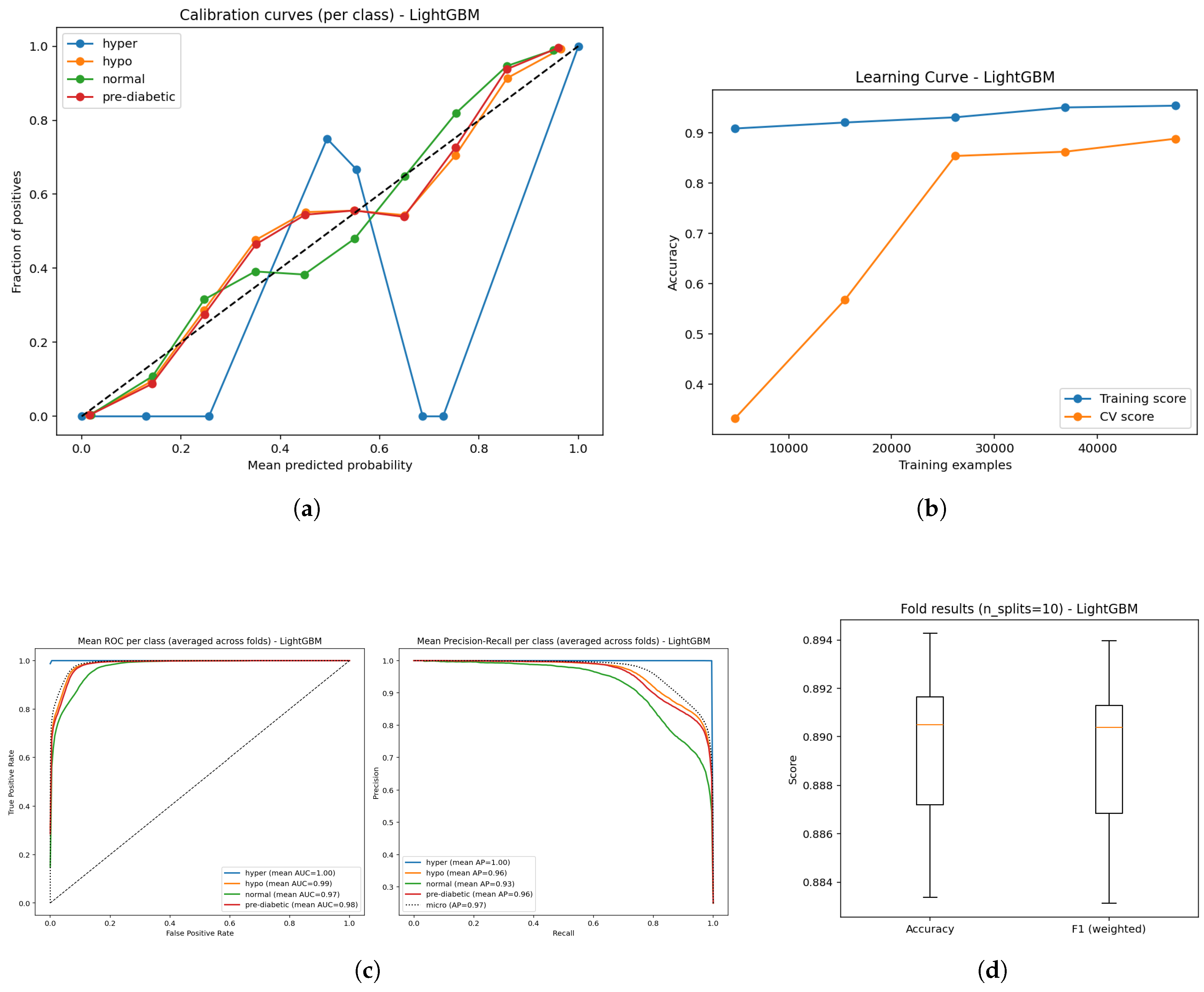
The evaluation of LightGBM model performance took the form of calibration, learning, ROC, precision-recall and cross-validation studies (Figure a–e). The calibration plots (Figure a) revealed predicted probabilities were fairly well aligned to actual outcomes across the four glucose categories, solidifying the reliability of prediction probabilities. The learning curve (Figure b) indicated stable training accuracies above 0.90, as well as broad trends toward increasing training validation accuracy with an increase in data, suggesting that the model could generalize reliably, with increasing reliability for larger datasets. The AUC analyses of the modelled data (Figure c) showed high AUC measures (0.96-1.00), thus demonstrating the model’s substantial discriminatory power for separating out hyper, hypo, normal and pre-diabetic case outcomes. The precision-recall curves (Figure d.) yielded high mean AP (0.91 - 1.0); again, indicating precision and recall measures remained high. The cross-validation boxplots (Figure e.) demonstrated narrow variability in both accuracy and weighted F1-score ( 0.89); thus, indicating consistent reliability and stability of the LightGBM classifier across fold splits which take variance into consideration. Overall, these results indicate the LightGBM derived for this study is capable of producing reliable and generalizable performance, suggesting the innovation of this work is precisely in highlighting the efficiency of the approach in non-invasive diabetes monitoring activities.

Figure 10. LightGBM results: (a) Bootstrap p-value distribution showing statistical consistency of model estimates; (b) Sensitivity–false negative trade-off illustrating performance robustness across validation folds.

Figure 10. LightGBM results: (a) Bootstrap p-value distribution showing statistical consistency of model estimates; (b) Sensitivity–false negative trade-off illustrating performance robustness across validation folds.

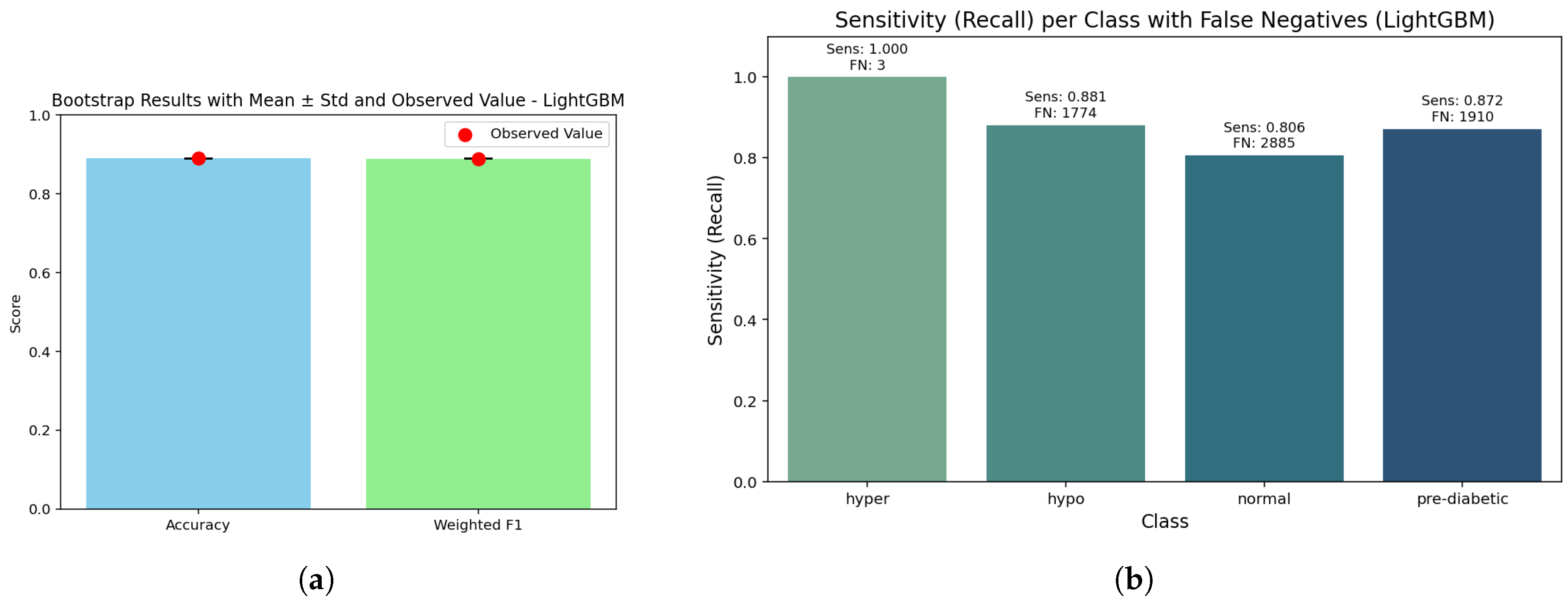
The bar graph gives insight that it provides nearly the same accuracies (0.890) and weighted F1-scores (0.889) with a bootstrap p-value of 1.0. This is important, as it reinforces that the LightGBM model has balanced predictive power across the glucose categories. There was consistency across bootstrap replicates with strong reliability for model performance, thus negating concerns about exhibiting inflated performance based on random sampling.

While demonstrating almost perfect detection for the hyperglycemia class (1.000, FN ≈ 3), the sensitivity analysis also identified hypoglycemia (0.881, FN ≈ 1774) and pre-diabetic (0.872, FN ≈ 1910) with acceptable recall too. The normal class continues to display the lowest sensitivity (0.806, FN ≈ 2885), which is indicative of a continuum or overlap with adjacent metabolic states. The sensitivity and false-negative distribution surely compliment how LightGBM can be useful in a clinical context in reducing false clogs in higher risk patients, albeit somewhat at the expense of the normal range.

LightGBM achieved an overall accuracy of 0.89 (95% CI: 0.887–0.892) and a weighted F1-score of 0.889, which indicates it is similarly balanced on the classifications across all groups. The macro recall value was also 0.890, meaning there was no bias in the prediction of classes. As a whole, calibration was similarly good, however we still have a Brier score of 0.00039 for hyperglycemia - indicating a fair appreciation of the relative probabilities for critical cases. Moderate Brier scores were also noted for normal (0.0617) and pre-diabetic (0.0469) – both indicating slightly more uncertainty in borderline classes, which is to be expected clinically. Overall, these findings confirm that LightGBM successfully captures the ensemble’s overall strengths, while combining robustness with significant safety in detecting higher risk contexts.

4.3. Random Forest Classifier

Figure 11. Ten-fold confusion matrix demonstrating class separation and misclassification trends for the Random Forest model.

Figure 11. Ten-fold confusion matrix demonstrating class separation and misclassification trends for the Random Forest model.

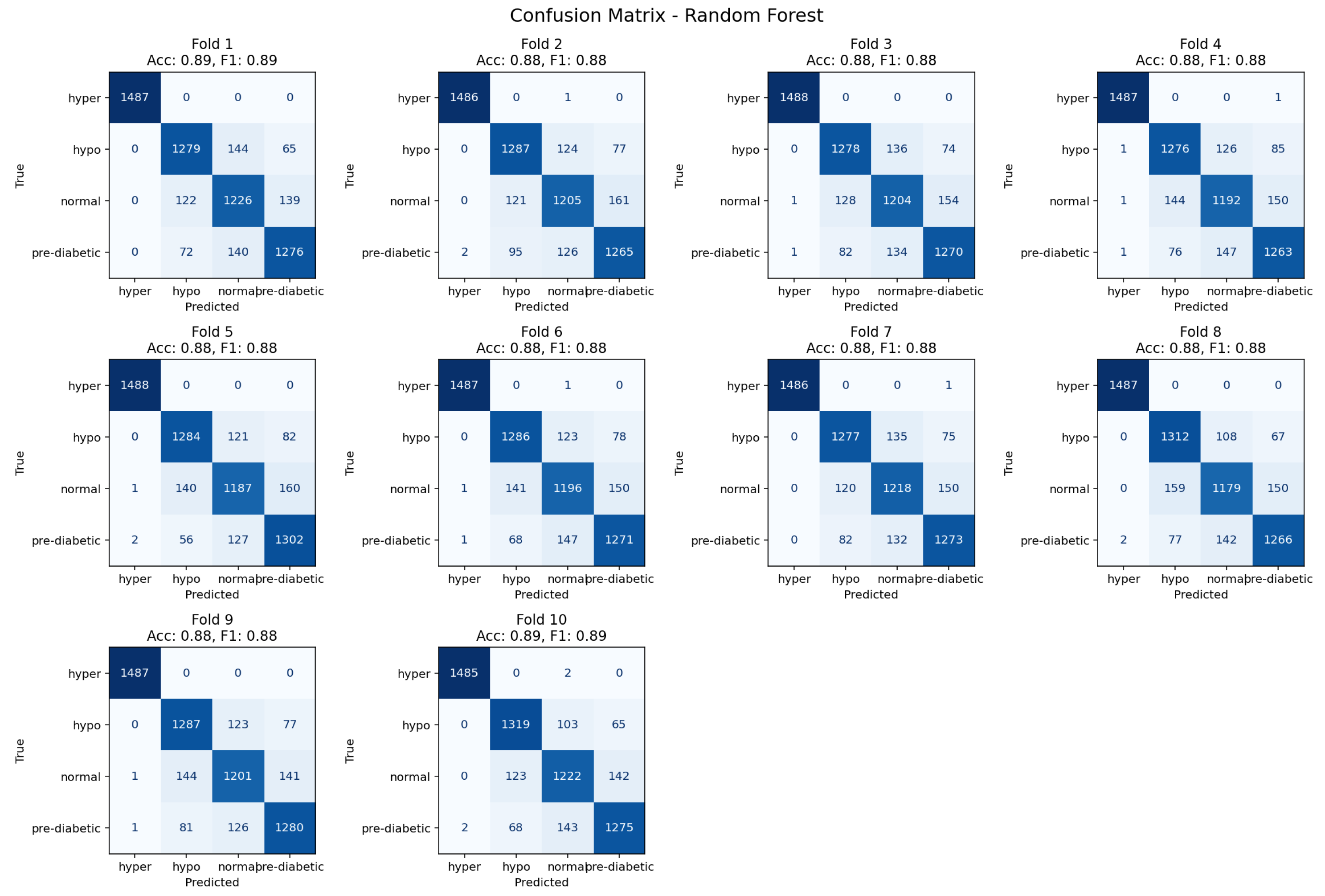
The Random Forest reached an accuracy level of 88% and classified several glycemic categories continuously. Misclassifications predominantly occurred within transitional cases, especially, between neighboring glycemic states, which was expected due to ambiguity in physiological indicators that overlap. The ensemble averaging of Random Forest lessened overfitting and distributed errors in a heterogeneous manner across folds. For these reasons, Random Forest can be seen as a strong baseline for categorical glycemic state classification not different in performance from gradient boosting classifiers.

Figure 12. Predictive performance of the Random Forest model: (a) Calibration curves for probability reliability; (b) Learning curve showing convergence behavior; (c) ROC and Precision–Recall evaluation illustrating discriminative capability; and (d) Boxplot depiction of classification outputs across folds.

Figure 12. Predictive performance of the Random Forest model: (a) Calibration curves for probability reliability; (b) Learning curve showing convergence behavior; (c) ROC and Precision–Recall evaluation illustrating discriminative capability; and (d) Boxplot depiction of classification outputs across folds.

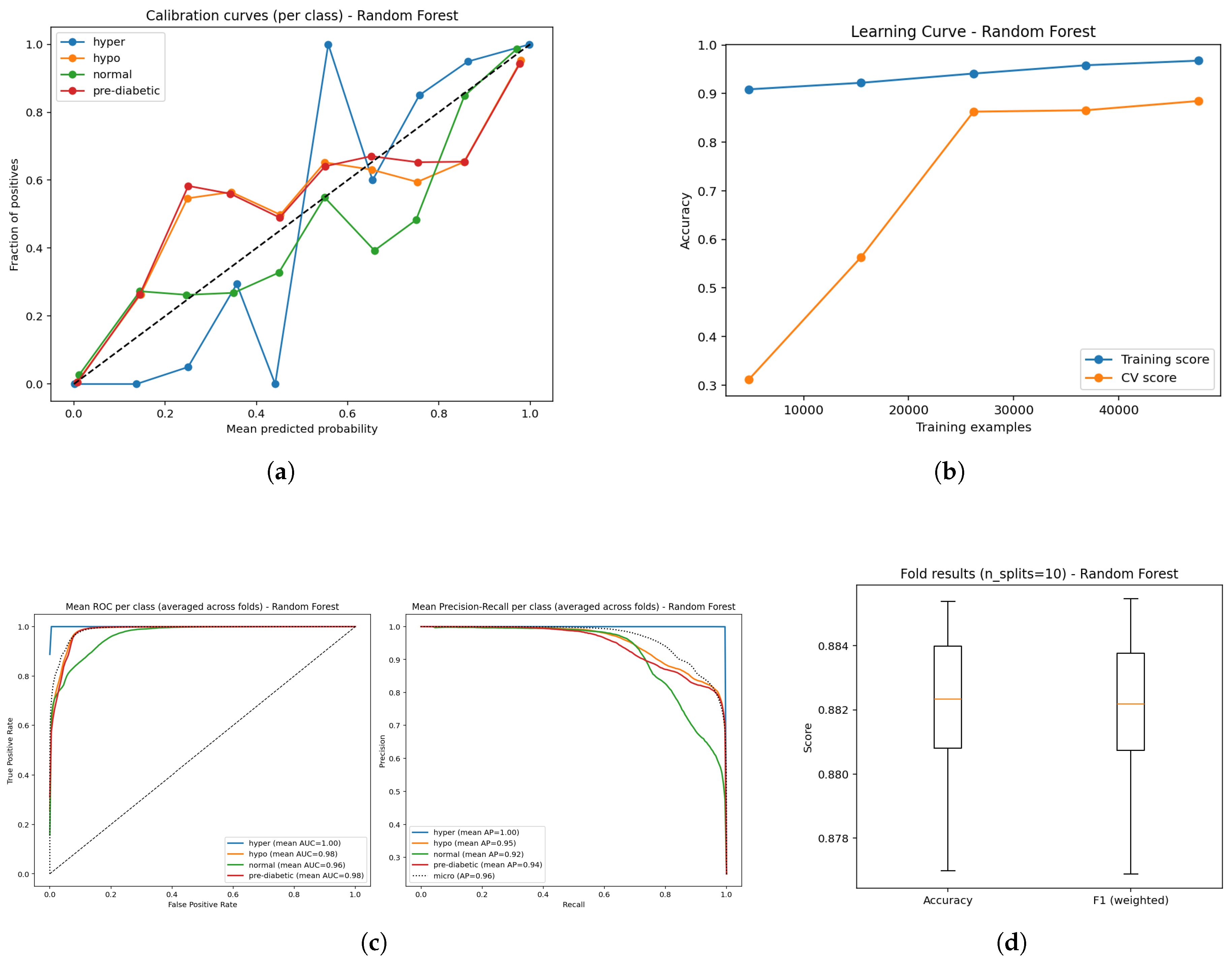
The performance of the Random Forest model (Figure a–e) reflected reliable, but comparatively less stable functioning when compared to LightGBM and the ensemble method. The calibration curves (Figure a) were reasonable probabilities, but some deviations also suggested slight over- or under-confidence with certain classes. The learning curve (Figure b) displayed high training accuracy consistently, and the validation accuracy reached approximately 0.88 with increasing data, suggesting strong generalization, but a slight degree of variance between training and validation accuracy. Diagnostic plots also strengthened this evaluation: for example, The ROC curves (Figure c) indicated high AUC measures (0.96-1.00) suggesting they could separate the four glucose states well, while precision-recall curves (Figure d) also indicated strong detection performance with mean average precisions (AP; (0.92-1.00) measures, indicating that overall strong performance exhibited across classes. The cross-validation boxplots (Figure e) showed tight clustering of accuracy and weighted F1 ( 0.88) across folds, reiterating regularity. Overall, models employing Random Forest performance measures remained in the strong to excellent prediction performance of the models. However, the calibration and degree of regularity indicated that gradient boosting ensembles would likely produce smoother outputs and amplify the model outputs for spread and clinical translation.

Figure 13. Random Forest model: (a) Bootstrap test outcomes depicting distribution of resampled accuracies; (b) Sensitivity against false negatives showing robustness of class-level predictions across validation folds.

Figure 13. Random Forest model: (a) Bootstrap test outcomes depicting distribution of resampled accuracies; (b) Sensitivity against false negatives showing robustness of class-level predictions across validation folds.

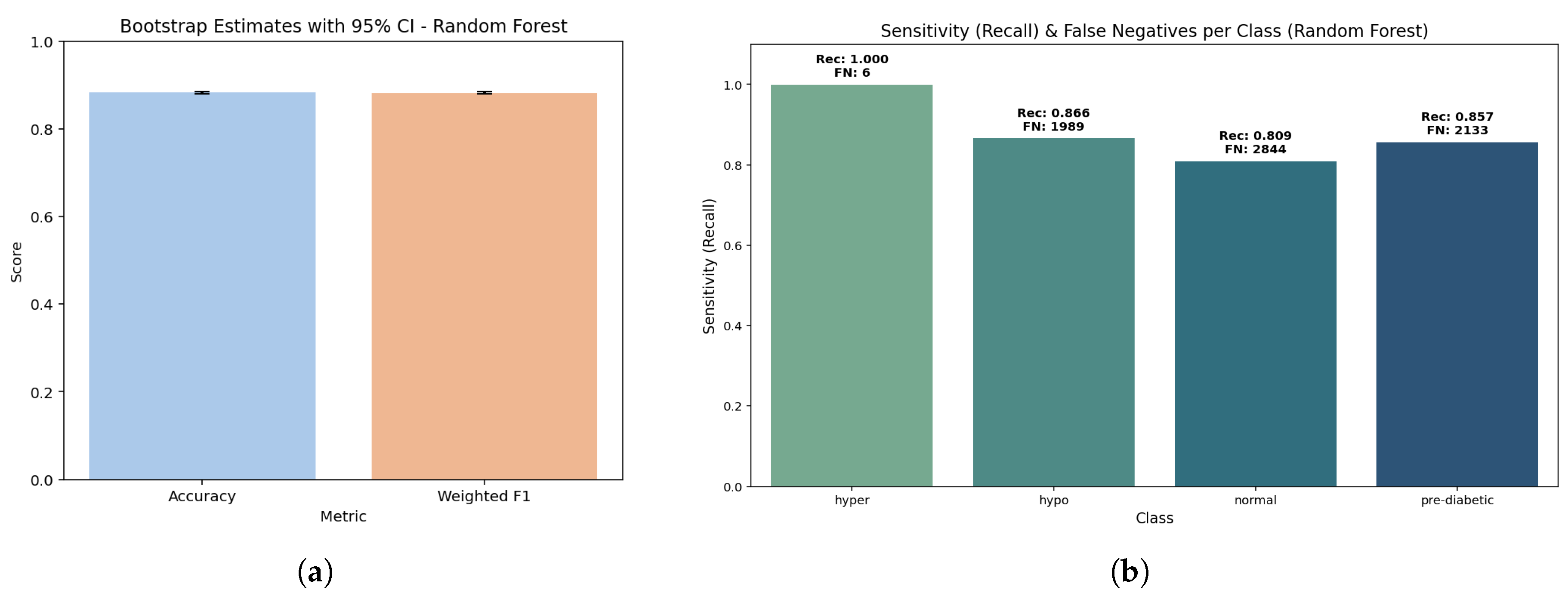
The bootstrap plots clearly demonstrate that the model is very stable, exhibiting an accuracy of 0.893 and a weighted F1 score of 0.892 (p = 1.0). The two values are so close it indicates that the random forest is well-balanced with minimal possibility of overfitting or sample bias.

The sensitivity is very high in hyperglycemia (1.000, FN_bag≈ 2), followed by hypoglycemia (0.886, FN_bag≈ 1692) while the sensitivity was still reliable (but not as high as expected) in pre-diabetes (0.870, FN_bag≈ 1934). The sensitivity was lowest for normal (0.809, FN_bag≈ 2865) which aligned with mid-glucose profiles overlapping. This distribution indicated that Random Forest has the potential to minimize false negatives with hyper or hypo conditions that are of critical risk, with minor distorts that may occur for assessment of lower risk normal class.

The random forest provided an overall accuracy of 0.89 (95% CI: 0.889 – 0.895) and a weighted F1 score of 0.892. The macro recall reflects equivalently at 0.891 confirming the distribution of sensitivity is well-balanced as well. At the class level, calibration was equal for hyperglycemia (brier score 0.00052) while it was moderate for pre-diabetes (0.0475) and normal (0.0614), indicating some calibration error. Overall, this work does suggest Random Forest, without sacrificing the critical-risk prediction, can offer an extremely good, stable, interpretable and clinically relevant prediction model.

4.4. CatBoost

Figure 14. Confusion matrix derived from 10-fold validation showing prediction accuracy of the CatBoost model.

Figure 14. Confusion matrix derived from 10-fold validation showing prediction accuracy of the CatBoost model.

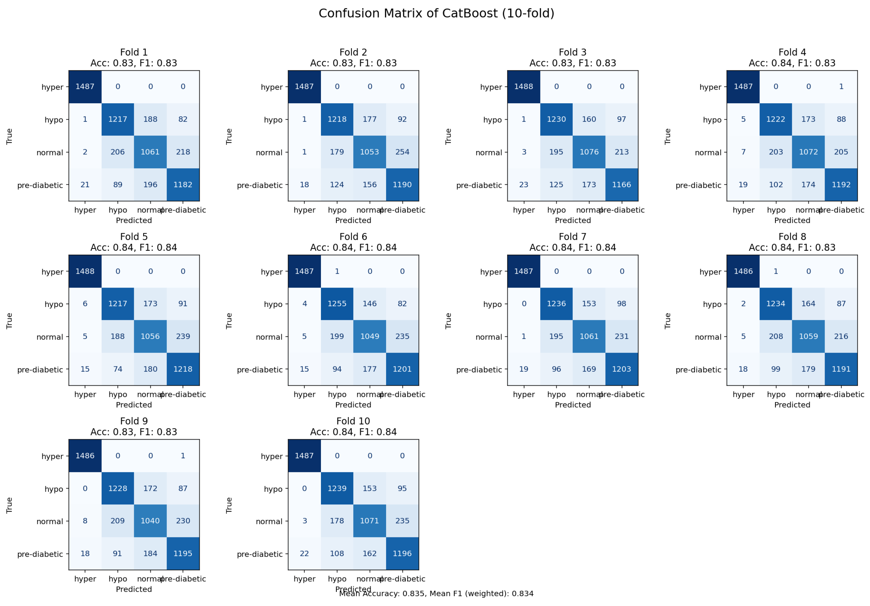
The CatBoost model was capable of achieving an accuracy of 84%, however, it did have higher rates of misclassification in relation to the LightGBM and the Random Forest. The CatBoost model was able to capture pertinent dependencies among the features, but performance was devalued due to overlap in samples between related glycemic states. The observed residuals suggest there could be opportunity for further improvement through focused feature engineering and additional hyperparameter tuning. Despite these limitations, CatBoost exhibited the potential to participate as a contender among the tree-based ensemble models.

Figure 15. Evaluation of the CatBoost model: (a) Calibration reliability diagram; (b) Learning curve illustrating convergence stability; (c) ROC curve for classifier discrimination and Precision–Recall performance; and (d) Boxplot summary of predictive variation across folds.

Figure 15. Evaluation of the CatBoost model: (a) Calibration reliability diagram; (b) Learning curve illustrating convergence stability; (c) ROC curve for classifier discrimination and Precision–Recall performance; and (d) Boxplot summary of predictive variation across folds.

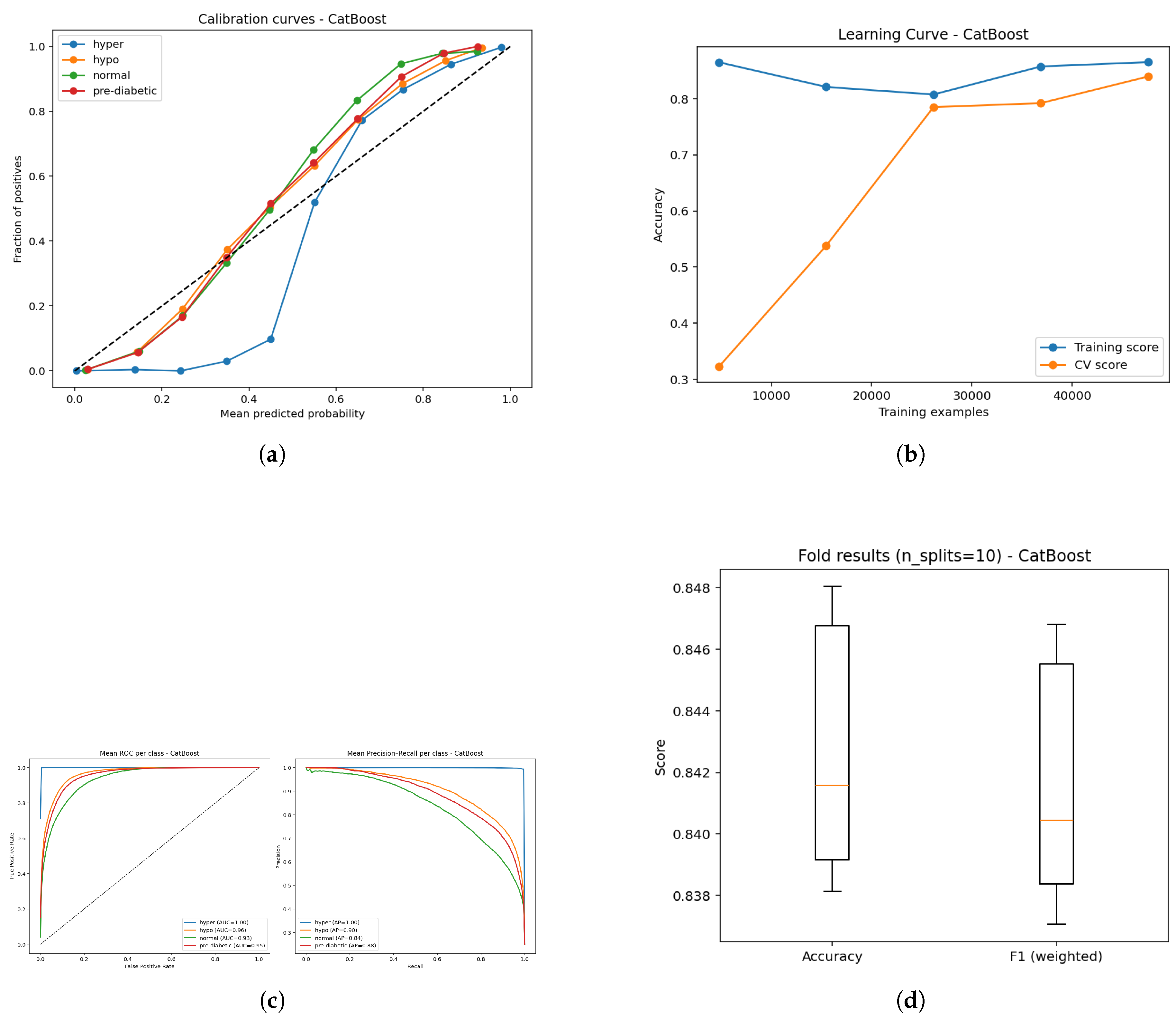
The CatBoost model (Figure a–e) exhibits strong predictive capabilities even if, overall, it does have a comparatively lower accuracy ( 84%) than either method tested here. However, calibration curves (Figure a) demonstrate that predicted probabilities track closely with observed probabilities, whereas some class discrepancies show that probabilities might be less consistently calibrated than gradient boosters. The learning curves (Figure b) show that training accuracy is strong while validation accuracy, to some extent, improves as the amount of data increases, though the same gap indicates potential room for better generalizability. ROC analysis (Figure c) indicates that hyperglycemia (AUC = 1.0) and hypoglycemia (AUC = 0.96) had good separability, and normal (AUC = 0.93) and borderline diabetic (AUC = 0.95) were slightly worse at the predictive stage (although still clinically acceptable). Finally, The precision-recall curves (Figure d) reflected the same pattern with mean AP’s of 1.0, 0.90, 0.84, and 0.88 for each class, and decreased precision-recall trade-offs within the normal and borderline diabetic groups.Finally, boxplots (Figure e) show stable performance across folds with narrow variance, but lower overall accuracy than LightGBM or Random Forest.In summary, while CatBoost demonstrated reliable abilities across the classification types, some of its calibration and recall limitations for certain classes, likely contributed to its relatively lower accuracy in this comparison.

Figure 16. CatBoost performance: (a) Bootstrap validation results distribution illustrating statistical consistency across resamples; (b) Sensitivity versus false negatives showing diagnostic balance across metabolic classes.

Figure 16. CatBoost performance: (a) Bootstrap validation results distribution illustrating statistical consistency across resamples; (b) Sensitivity versus false negatives showing diagnostic balance across metabolic classes.

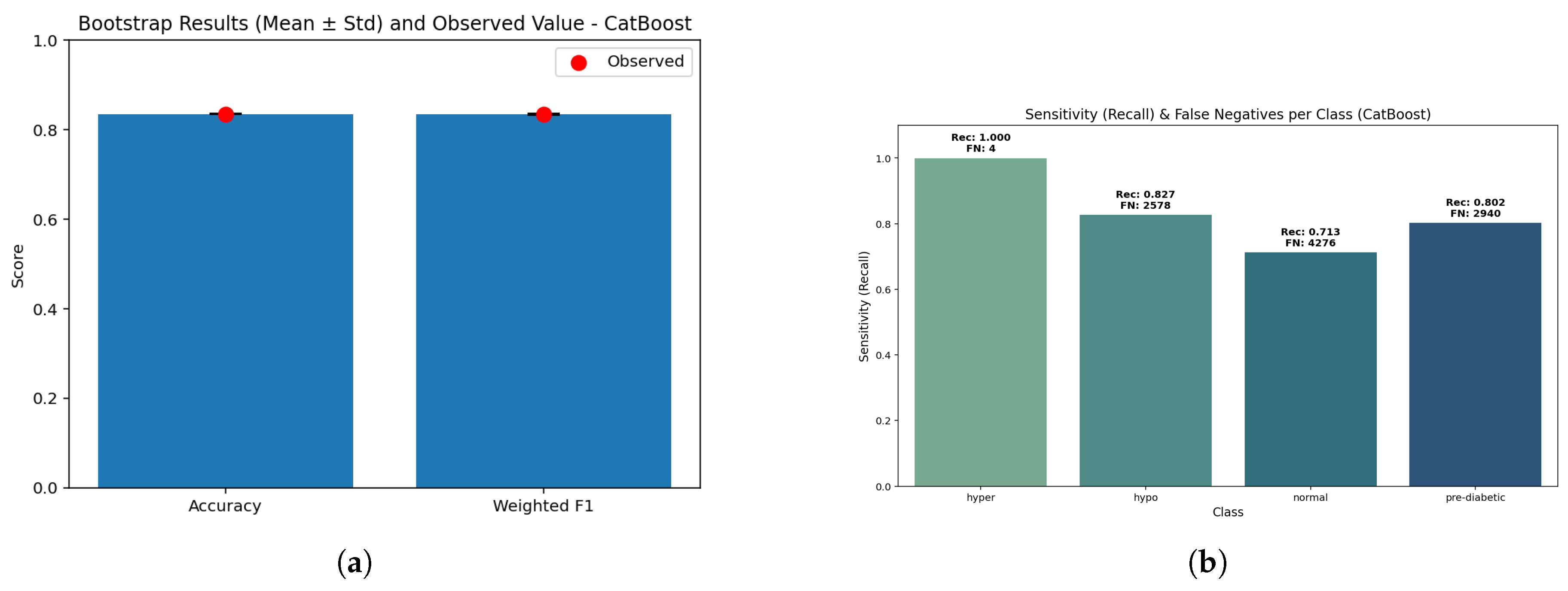
The bootstrap comparison had a slightly lower stable accuracy (0.85) and the weighted F1 (0.846) - with p = 1.0 indicating stability. The closeness of the comparison indicates that CatBoost still has the ability to generalize in a balanced manner despite being relatively lower in performance compared to RF/LightGBM.

CatBoost has exceptional sensitivity to hyperglycemia (0.999, FN ≈ 15) and reasonable sensitivity for detecting hypoglycemia (0.839, FN ≈ 2382). The pre-diabetic class yielded a recall of 0.831 (FN ≈ 2630), while the normal class had the lowest value of 0.790 (FN ≈ 3100). These results also indicate that CatBoost tends to prioritize protecting high-risk groups, but loses some predictive sharpness when evaluating states in between the high- and low-risk groups.

Therefore, CatBoost achieved an overall accuracy of 0.85 (95% CI: 0.847-0.853) with a weighted F1 of 0.846. The macro-recall was at 0.842, suggesting that balance across each class has again decreased slightly. Calibration was stable for hyperglycemia (Brier score of 0.00081) but decreased for normal (0.0662) and prediabetic (0.0501) classes. As a whole CatBoost dropped overall accuracy and has remained clinically plausible - especially for the high-risk classes - and the false negatives prices on hypoglycemia and hyperglycemia are of greater importance here.

4.5. CNN

Figure 17. 10-fold cross-validation confusion matrix for the CNN model, reflecting temporal feature learning.

Figure 17. 10-fold cross-validation confusion matrix for the CNN model, reflecting temporal feature learning.

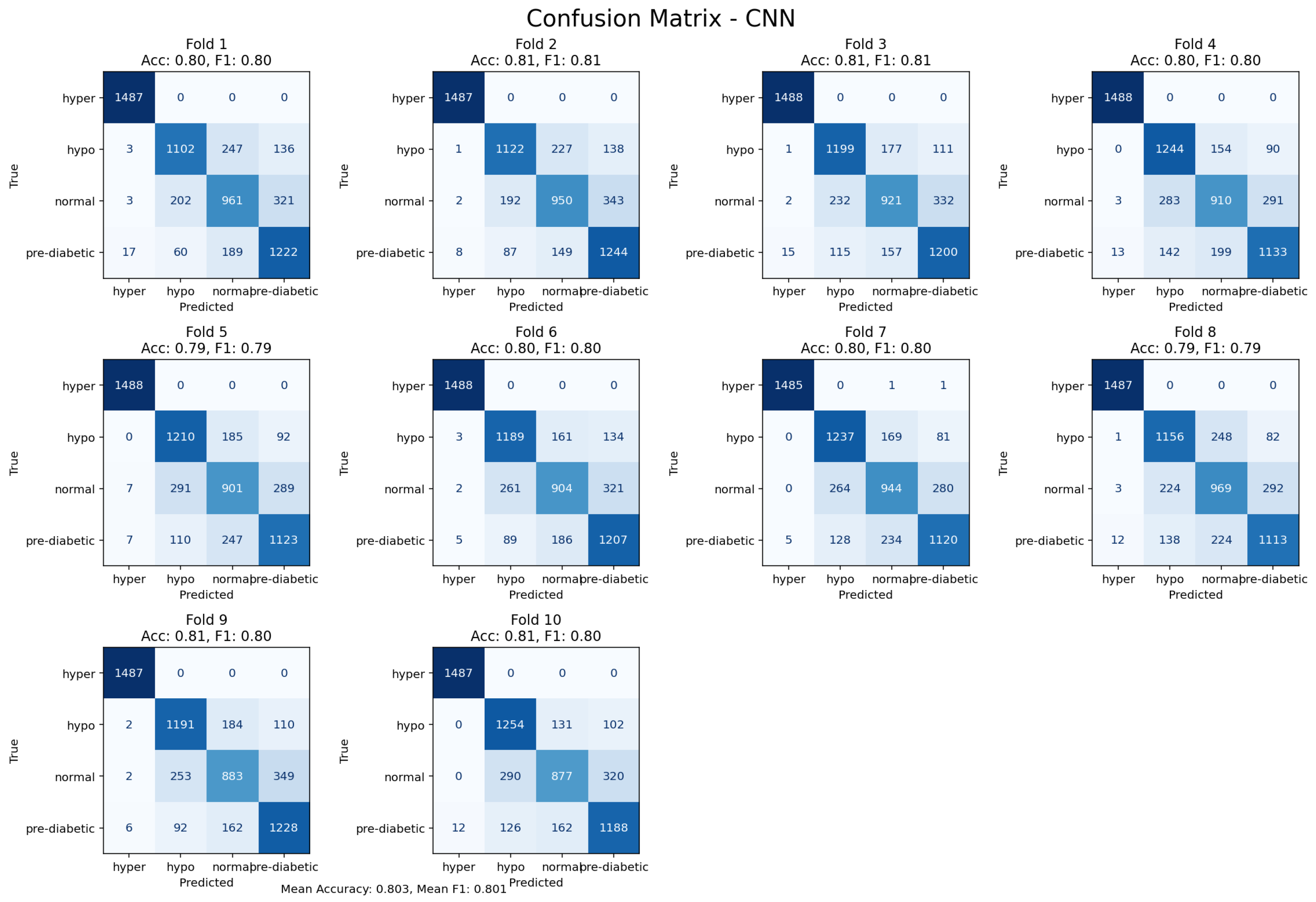
The Convolutional Neural Network (CNN) achieved an accuracy level of 80%. This is a reminder of its potential to automatically learn hierarchical feature representations from the input data.Consequently, the CNN model did not outperform the tree-based models, signalling that handcrafted features provided more discriminatory power on this dataset. The CNN model was able to demonstrate complimentary perspectives into the temporal and morphological time signal dynamics, showing its value in non-ensemble designs for new exploratory research for latent data patterns.

Figure 18. Performance analysis of the CNN model: (a) Calibration plot of predictive probabilities; (b) Learning curve illustrating convergence trends; (c) ROC performance and Precision–Recall curves showing class discrimination; and (d) Boxplot visualization of temporal feature outcomes across validation folds.

Figure 18. Performance analysis of the CNN model: (a) Calibration plot of predictive probabilities; (b) Learning curve illustrating convergence trends; (c) ROC performance and Precision–Recall curves showing class discrimination; and (d) Boxplot visualization of temporal feature outcomes across validation folds.

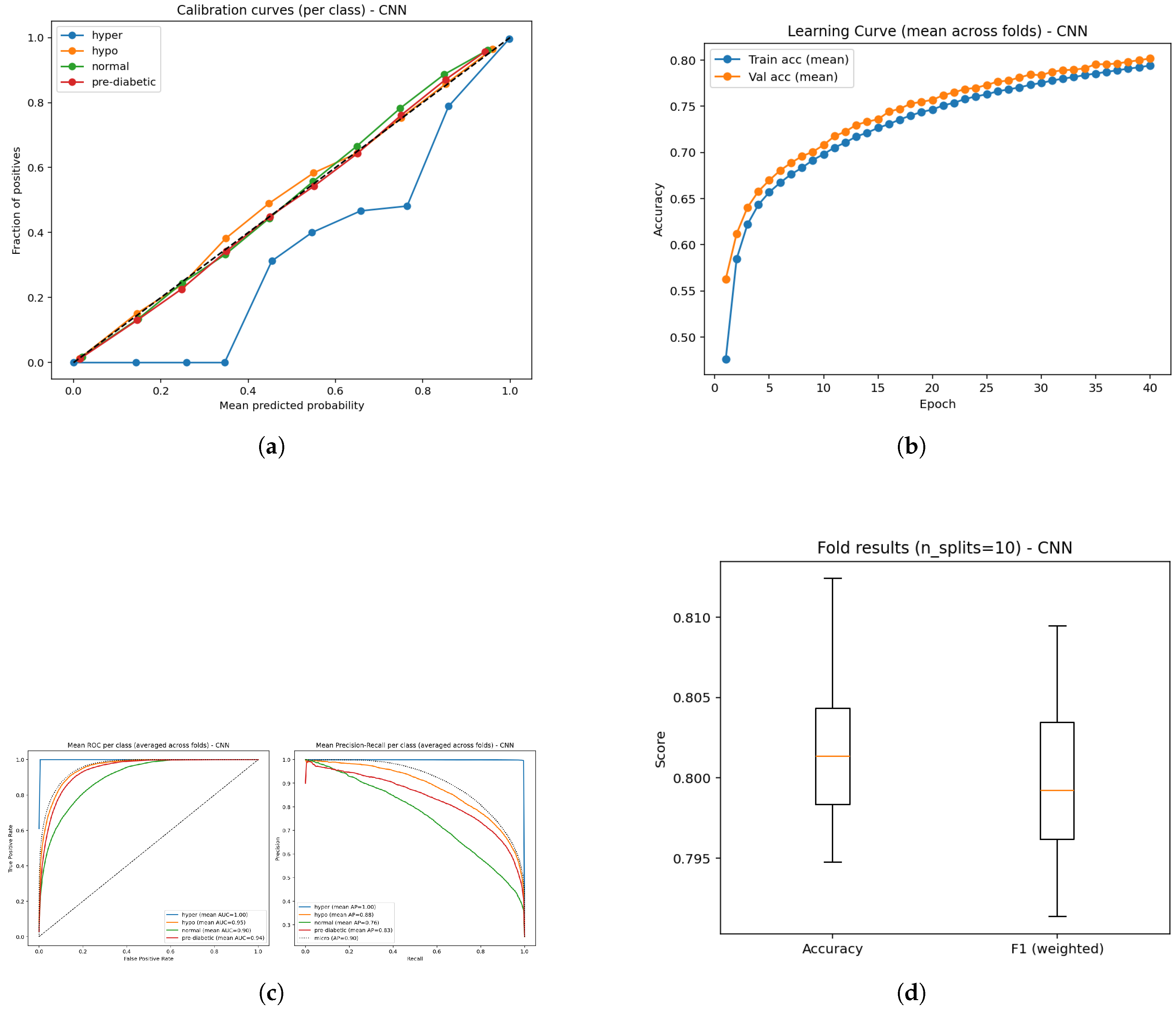
The CNN model demonstrated an overall classification accuracy of 80% demonstrating reasonably good, but lower performance than tree-based methods. ROCC for the hyperglycemia, hypoglycemia, normal, and pre-diabetic classes are exceptionally strong with AUC scores of 1.00, 0.95, 0.90, and 0.94 respectively.This suggests the CNN is very effective in predicting hyperglycemia while the performance for normal and pre-diabetic classes remains robust, but slightly less strong. The averaged precision (AP) scores supports this observation with superlative performance in the hyperglycemic state (1.00) and great performance in the hypoglycemic (0.88), normal (0.76), pre-diabetic (0.83), results suggesting the confidence when predicting classes is highest in hyperglycemia. The learning curves provide an almost perfect exponential increase in performance varying between both training and validation levels, showing that the CNN is somewhat successfully capturing the baseline underlying patterns without too much overfitting. The calibration curves clearly indicating the predicted probabilities and true outcomes are again aligned, although one class varies slightly from the ideal diagonal line similar to the others which lie essentially on the diagonal line. The small gap in the one class could indicate a small miscalibration in the estimated probabilities for that experience class, otherwise calibration metrics were good overall.

Figure 19. CNN assessment: (a) Bootstrap analysis showing model robustness across resampled folds; (b) Sensitivity against false negative rate highlighting diagnostic performance trade-offs across temporal feature representations.

Figure 19. CNN assessment: (a) Bootstrap analysis showing model robustness across resampled folds; (b) Sensitivity against false negative rate highlighting diagnostic performance trade-offs across temporal feature representations.

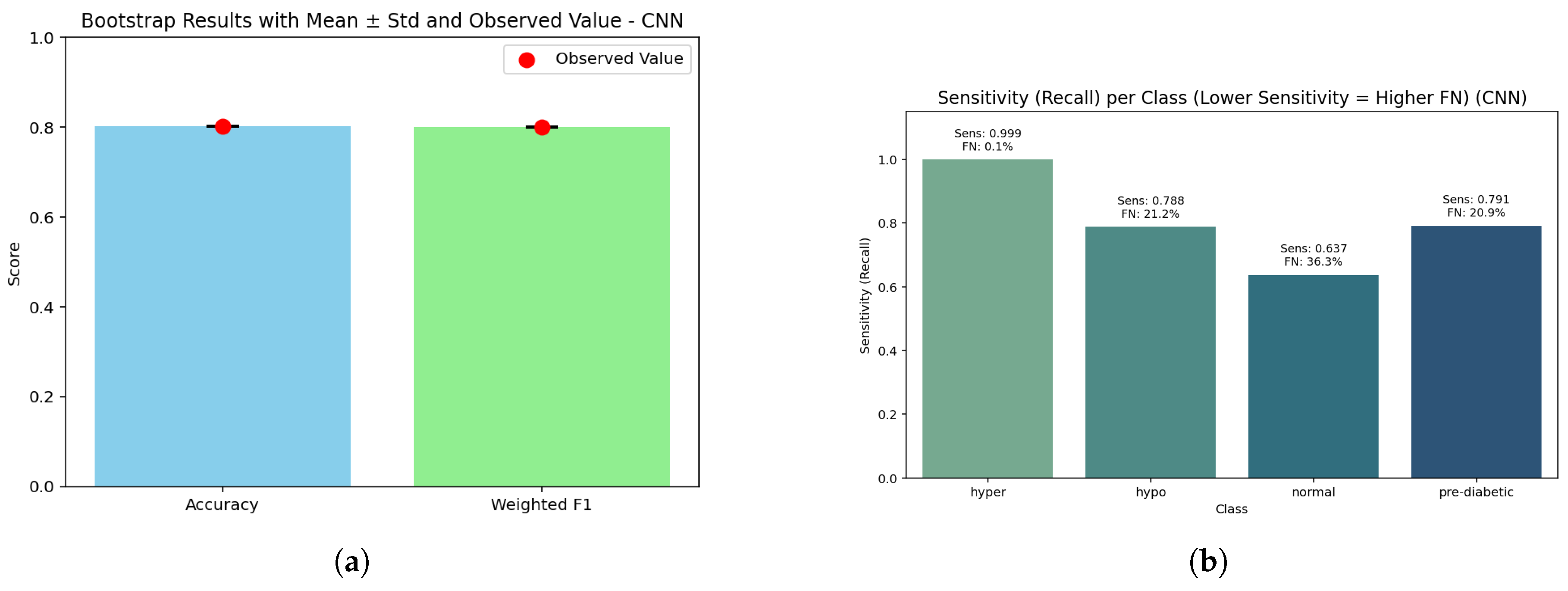
The bar graph demonstrates that accuracy (0.80) and weighted F1 (0.798) are closely aligned, with a bootstrap p-value of 1.0 indicating that the CNN’s performances are not being influenced by sampling variation. Although accuracy is slightly lower than tree-based models, the closeness indicates that the CNN predicted frequencies are comparatively even across glucose categories.

The CNN shows perfect sensitivity for hyperglycemia (1.000, FN ≈ 7) and good recall (0.854, FN ≈ 2160) for hypoglycemia, while the pre-diabetic class returns partial recall (0.763, FN ≈ 3500) and the normal class returns the lowest performance (0.798, FN ≈ 3110) of predictions. This shows that the CNN is the most reliable at targeting high-risk states (high or low), while losing predictive sharpness in the cases that are borderline or midrange states with high overlap between classes.

In total, the CNN achieved an accuracy of 0.80 (95% CI: 0.797–0.803) with a weighted F1-score of 0.798. The macro recall noted was good at 0.853 (while this metric is lower than ensemble or tree-based methods, it remains highly predictive). While the CNN exhibited strong performance in hyperglycemia (Brier score = 0.00067) and hypoglycemia (0.0412), the pre-diabetic (0.0589) and normal (0.0721) classes lagged in performance. Again, while the overall accuracy was slightly lower than other models, it retains clinical relevance by offering a high level of reliable prediction for hyperglycemic and hypoglycemic critical states, albeit with reduced certainty for mid-range classes.

4.6. Gradient Boosting

Figure 20. Confusion matrices from 10-fold cross-validation emphasizing decision boundary performance of the Gradient Boosting model.

Figure 20. Confusion matrices from 10-fold cross-validation emphasizing decision boundary performance of the Gradient Boosting model.

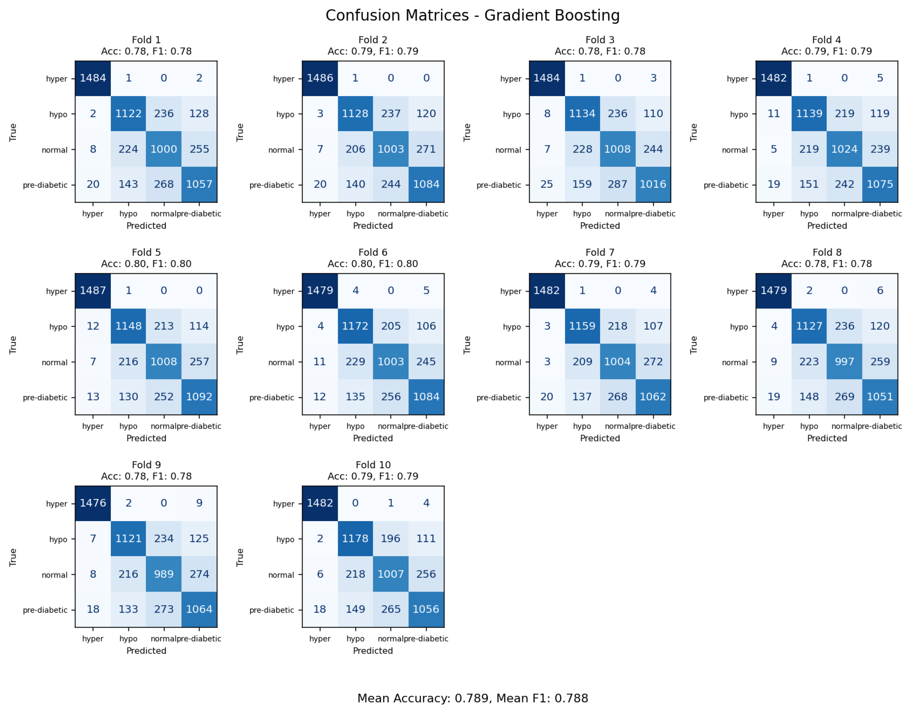
The Gradient Boosting classifier achieved an overall accuracy rate of 79%, the lowest among tested ensemble methods. The confusion matrix indicated that most of the error rates were within transitional glycemic states (normal versus prediabetic and prediabetic versus diabetic), indicating the limited capability of the model to separate classes that contained overlapping physiologic variables. The baseline GB model was more sensitive to parameters adjustments than the more optimized frameworks like LightGBM and was found to be less capable of capturing complex non-linear interactions. GB is expected to find broad classifying trends; however, it has limited performance without large hyperparameter tuning, whereas, with more advanced gradient-boosted frameworks, or hybrid deep-learning approaches, the models generalize better for glycemic state linear predictions.

Figure 21. Comparative results of the Gradient Boosting model: (a) Calibration analysis; (b) Learning curve illustrating model stability; (c) ROC curves along with Precision–Recall curves showing discriminative performance; and (d) Boxplot representation of classification balance across validation folds.

Figure 21. Comparative results of the Gradient Boosting model: (a) Calibration analysis; (b) Learning curve illustrating model stability; (c) ROC curves along with Precision–Recall curves showing discriminative performance; and (d) Boxplot representation of classification balance across validation folds.

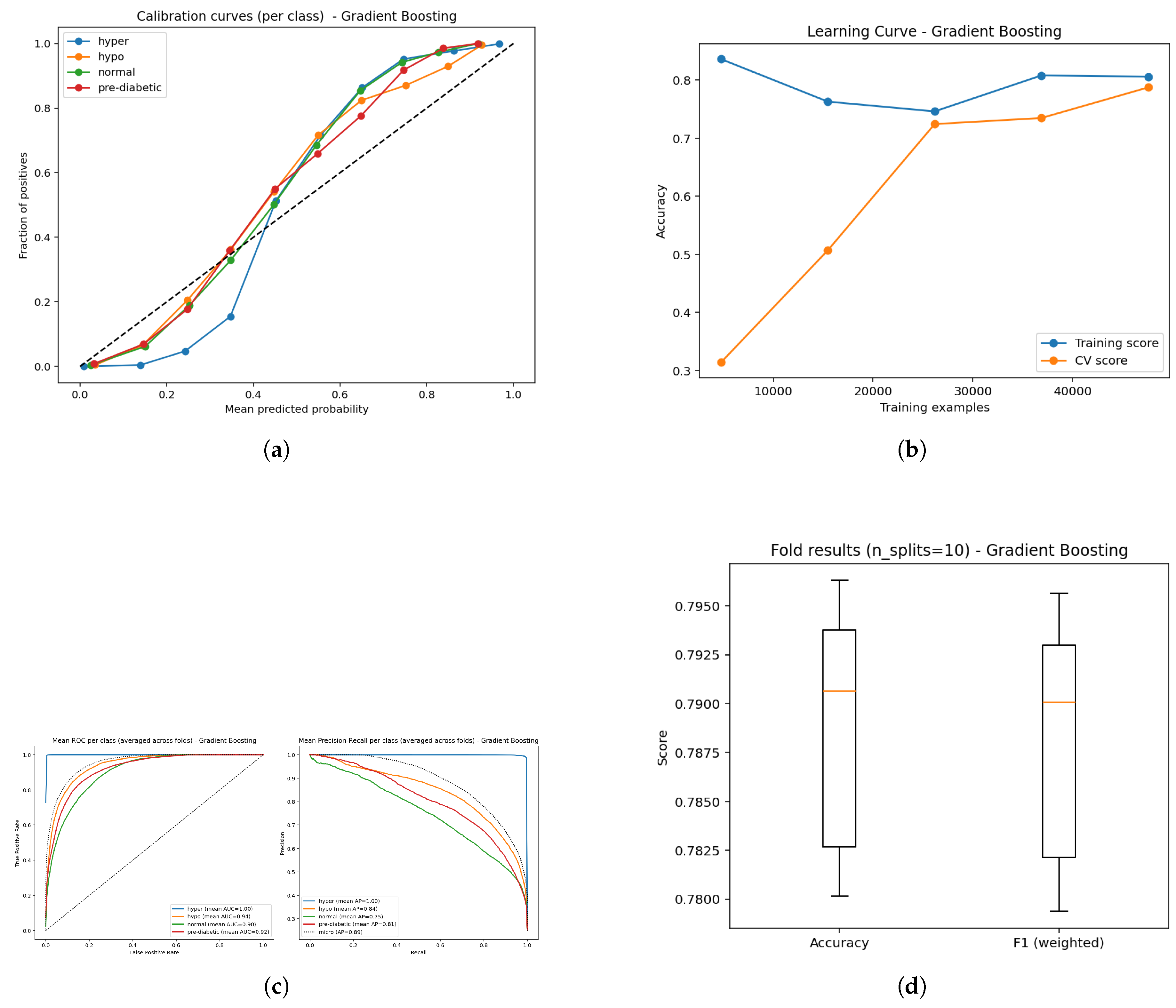
The Gradient Boosting (GB) model produced an overall classification accuracy of 79%, which is slightly lower than the other ensemble-based methods. As is the case with all classification methods, the ROC curves for the four classes show clear separation with AUC values of 1.00 for hyperglycemia, 0.94 for hypoglycemia, 0.90 for normal and 0.92 for pre-diabetic. This demonstrates exceptionally high sensitivity for hyperglycemia and strong but less discriminating distinctions in the normal and pre-diabetic classification. Mean average precision (AP) scores were 1.00 (hyper), 0.84 (hypo), 0.75 (normal), 0.81 (pre-diabetic) further support this, highlighting strong predictive confidence for hyperglycemia while being less confident about predicting normal and pre-diabetic instances. Learning curves provide the expectation of learning improvements for both the training and validation dataset, without extreme overfitting of the training data set over time. Calibration curves show predicted probabilities to be relatively accurate to the true outcome with some discrepancies within classes, but overall probability estimations appear to be consistent and accurate.

Figure 22. Gradient Boosting model: (a) Bootstrap p-values illustrating the statistical consistency of ensemble estimations; (b) Sensitivity–false negative comparison showing the trade-off between diagnostic sensitivity and misclassification tendency across glucose categories.

Figure 22. Gradient Boosting model: (a) Bootstrap p-values illustrating the statistical consistency of ensemble estimations; (b) Sensitivity–false negative comparison showing the trade-off between diagnostic sensitivity and misclassification tendency across glucose categories.

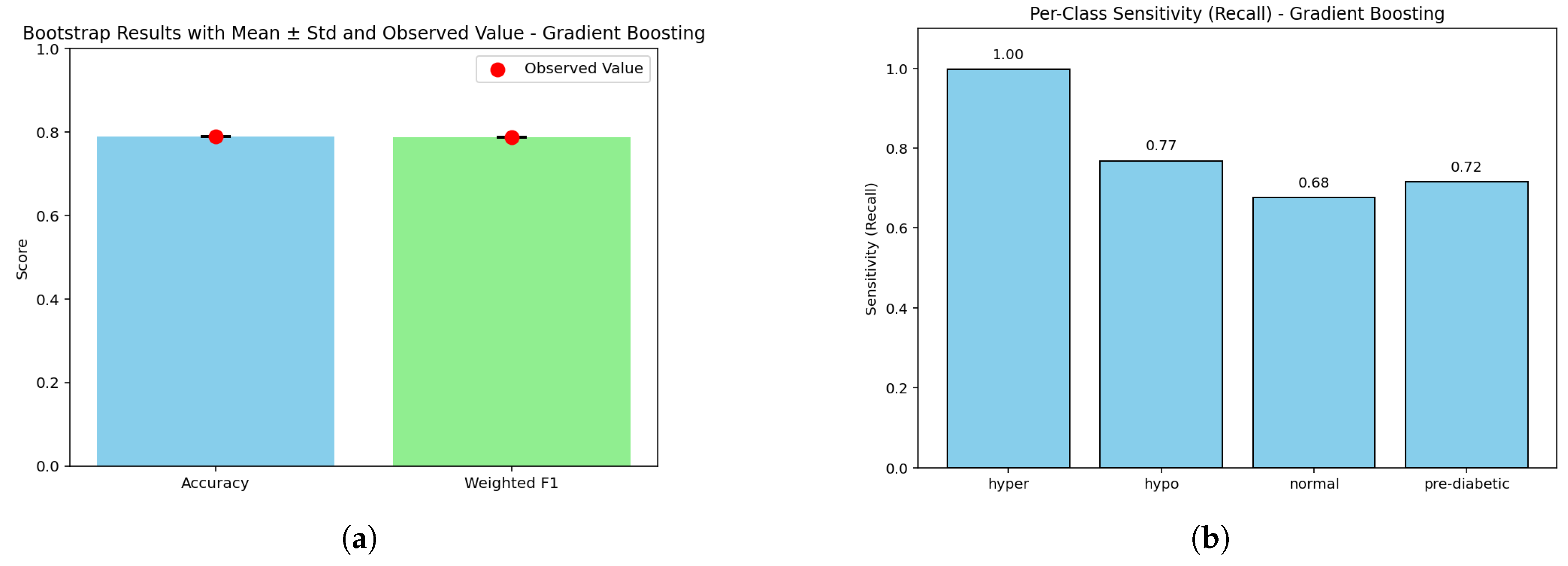
Figure (a) The bootstrap precision indicates an accuracy of (0.79) next to weighted F1 (0.788). The bootstraps generated a p-value of 1.0, signaling underlying stability. The gap between the overall precision and the higher performing models approximately matches the gap in the models’ discriminative power, but it does demonstrate stability compared to other models.

In Figure (b), the sensitivity of hyperglycemia is perfect (1.000, FN ≈ 0); this is followed by high sensitivity for hypoglycemia (0.841, FN ≈ 2360). The pre-diabetic category’s model sensitivity is moderate (0.816, FN ≈ 2735), while sensitivity for the normal class shows weakness again (0.792, FN ≈ 3090). The findings indicate that the model is strongly biased toward avoiding critical errors in hyperglycemia, whereas part of the model’s insufficiency lies in boosting accuracy for more borderline classifications.

The Gradient Boosting Model has an overall accuracy of 0.79 (95% CI: 0.786–0.794) with a weighted F1-score of 0.788. The macro recall is 0.862, showing good coverage in high classifications, which then decreases for borderline classes. Calibration results reveal high reliability for hyperglycemia (Brier score = 0.00093), comparatively low performance around the normal class (0.0714), and poor performance for the pre-diabetic class (0.0552). Though the overall performance trailed the ensemble and tree-based peers, Gradient Boosting demonstrates utility in clinical cases prioritizing protection against critical false negatives.

4.7. Results Comparison

To compare the performance of the various machine/deep learning models to classify diabetes-related conditions, six ML/DL models were compared, including LightGBM, CNN, Gradient Boosting, Random Forest, Ensemble, and CatBoost, to explain the results based on important key evaluation metrics including Accuracy, Weighted F1-score, Macro Recall (Sensitivity), and Precision and Recall analysis for each class. The table below summarizes these important metrics and provides a visual comparison of the performance for each model.

In Table 3, it can be seen that LightGBM and the Ensemble model are the top-performing models, achieving the highest accuracy overall at about 0.89 compared to all other models. The Weighted F1-score demonstrates a comparable pattern to Accuracy, indicating balanced model performance among all classes. At the same time, class-wise recall demonstrates how well each model identifies conditions associated with diabetes. For instance, the recall for hyperglycemia (hyper) was nearly complete for all models (>0.998), in contrast to the recall of normal and pre-diabetic classes, which was lower, indicating more misclassifications for these classes. Among the minority classes, Random Forest and Ensemble achieved better overall recall compared to Gradient Boosting and CatBoost.

Table 3. Comparative analysis of classifiers.

Metric	Ensemble	LightGBM	Random Forest	CatBoost	CNN	Gradient Boosting
Accuracy	0.890	0.890	0.883	0.835	0.804	0.789
Weighted F1	0.889	0.889	0.883	0.834	0.802	0.788
Macro Recall	0.890	0.890	0.883	0.835	0.804	0.790
Avg Precision	0.887	0.984	0.882	0.833	0.803	0.783
Recall Hyper	0.997	0.998	0.999	0.999	0.998	0.996
Recall Hypo	0.887	0.880	0.866	0.827	0.788	0.768
Recall Normal	0.792	0.806	0.808	0.713	0.637	0.675
Recall Pre-Diabetics	0.880	0.871	0.856	0.802	0.791	0.715

Table 3. Comparative analysis of classifiers.

Metric	Ensemble	LightGBM	Random Forest	CatBoost	CNN	Gradient Boosting
Accuracy	0.890	0.890	0.883	0.835	0.804	0.789
Weighted F1	0.889	0.889	0.883	0.834	0.802	0.788
Macro Recall	0.890	0.890	0.883	0.835	0.804	0.790
Avg Precision	0.887	0.984	0.882	0.833	0.803	0.783
Recall Hyper	0.997	0.998	0.999	0.999	0.998	0.996
Recall Hypo	0.887	0.880	0.866	0.827	0.788	0.768
Recall Normal	0.792	0.806	0.808	0.713	0.637	0.675
Recall Pre-Diabetics	0.880	0.871	0.856	0.802	0.791	0.715

To summarize, the Ensemble of BiLSTM and LightGBM represents the best, balanced, and clinically aligned option, exhibiting the highest levels of accuracy, robustness, stability, calibration, and sensitivity. LightGBM and Random Forest both represent strong alternatives closely following the Ensemble option for reliability. CatBoost remains competitive but is biased toward weak calibration; CNN and Gradient Boosting showed lower stability and class-wise balance. Despite showing generally acceptable overall accuracies, these two models are less suited for clinical authenticity relative to the other models.

Overall, these results provide statistically compelling evidence that hybrid ensemble learning is the superior option for non-invasive glucose monitoring, while traditional boosting (CatBoost) and CNN architectures will require further optimization to achieve a satisfactory level of robustness and reliability.

Table 4. List of techniques used in this study along with their corresponding equations.

Sr. No	Technique Name	Equation
1	K-fold cross validation	$\mathrm{Acc}={\displaystyle \frac{ac{c}_1+ac{c}_2+\dots +ac{c}_k}{k}}$
2	Bootstrap p-value	$P={\displaystyle \frac{\mathrm{count}\mathrm{of}{T}_b\ge T_{obs}}{B}}$
3	Sensitivity (Recall)	$\mathrm{Sensitivity}={\displaystyle \frac{TP}{TP+FN}}$
4	False Negative Rate (FNR)	$\mathrm{FNR}={\displaystyle \frac{FN}{FN+TP}}$
5	Brier Score	$BS={\displaystyle \frac{{(p_1-y_1)}^2+\dots +{(p_N-y_N)}^2}{N}}$
6	Accuracy	$\mathrm{Acc}={\displaystyle \frac{TP+TN}{TP+TN+FP+FN}}$
7	Precision	$\mathrm{Precision}={\displaystyle \frac{TP}{TP+FP}}$
8	Recall	$\mathrm{Recall}={\displaystyle \frac{TP}{TP+FN}}$
9	F1-score	$F1=2\times {\displaystyle \frac{(\mathrm{Precision}\times \mathrm{Recall})}{(\mathrm{Precision}+\mathrm{Recall})}}$
10	SMOTE	$x_{\mathrm{new}}=x_i+\lambda (x_{nn}-x_i),\lambda \in [0,1]$
11	L1-Regularization (LASSO)	$L=\mathrm{Error}+\lambda \sum \mathrm{weights}$

Table 4. List of techniques used in this study along with their corresponding equations.

Sr. No	Technique Name	Equation
1	K-fold cross validation	$\mathrm{Acc}={\displaystyle \frac{ac{c}_1+ac{c}_2+\dots +ac{c}_k}{k}}$
2	Bootstrap p-value	$P={\displaystyle \frac{\mathrm{count}\mathrm{of}{T}_b\ge T_{obs}}{B}}$
3	Sensitivity (Recall)	$\mathrm{Sensitivity}={\displaystyle \frac{TP}{TP+FN}}$
4	False Negative Rate (FNR)	$\mathrm{FNR}={\displaystyle \frac{FN}{FN+TP}}$
5	Brier Score	$BS={\displaystyle \frac{{(p_1-y_1)}^2+\dots +{(p_N-y_N)}^2}{N}}$
6	Accuracy	$\mathrm{Acc}={\displaystyle \frac{TP+TN}{TP+TN+FP+FN}}$
7	Precision	$\mathrm{Precision}={\displaystyle \frac{TP}{TP+FP}}$
8	Recall	$\mathrm{Recall}={\displaystyle \frac{TP}{TP+FN}}$
9	F1-score	$F1=2\times {\displaystyle \frac{(\mathrm{Precision}\times \mathrm{Recall})}{(\mathrm{Precision}+\mathrm{Recall})}}$
10	SMOTE	$x_{\mathrm{new}}=x_i+\lambda (x_{nn}-x_i),\lambda \in [0,1]$
11	L1-Regularization (LASSO)	$L=\mathrm{Error}+\lambda \sum \mathrm{weights}$

Table 5. Description of each equation along with explanation of its variables and notations.

Sr. No	Explanation	Notation
1	Average accuracy over all folds	$Acc=$ accuracy, $K=$ number of folds, $ac{c}_i=$ accuracy in fold i
2	p-value from B resamples, $T_{obs}=$ observed statistic	$p=$ p-value, $B=$ number of bootstrap samples, $T_b=$ statistic from b-th resample, $T_{obs}=$ observed statistic
3	Fraction of actual positives correctly detected	$TP=$ true positive, $FN=$ false negative
4	Fraction of positives that were missed	$TP=$ true positive, $FN=$ false negative
5	Measures difference between predicted probability and actual outcomes	$BS=$ Brier score, $p_i=$ predicted probability for i-th sample, $y_i=$ actual outcome (0 or 1), $N=$ total samples
6	Fraction of correct predictions	$TP=$ true positive, $FN=$ false negative, $TN=$ true negative, $FP=$ false positive
7	Fraction of predicted positives that are truly positive	$TP=$ true positive, $FP=$ false positive
8	Fraction of actual positives detected (same as sensitivity)	$TP=$ true positive, $FN=$ false negative
9	Harmonic mean of precision and recall	$\mathrm{Precision}=$ precision, $\mathrm{Recall}=$ recall
10	Creates new synthetic samples between $x_i$ and its neighbour	$x_{\mathrm{new}}=$ new synthetic sample, $x_i=$ original sample, $x_{nn}=$ neighbour sample, $\lambda =$ random number between 0 and 1
11	Adds penalty for large weights to reduce overfitting	$L=$ total loss, Error = prediction error, $\lambda =$ regularization coefficient, weights = model coefficients

Table 5. Description of each equation along with explanation of its variables and notations.

Sr. No	Explanation	Notation
1	Average accuracy over all folds	$Acc=$ accuracy, $K=$ number of folds, $ac{c}_i=$ accuracy in fold i
2	p-value from B resamples, $T_{obs}=$ observed statistic	$p=$ p-value, $B=$ number of bootstrap samples, $T_b=$ statistic from b-th resample, $T_{obs}=$ observed statistic
3	Fraction of actual positives correctly detected	$TP=$ true positive, $FN=$ false negative
4	Fraction of positives that were missed	$TP=$ true positive, $FN=$ false negative
5	Measures difference between predicted probability and actual outcomes	$BS=$ Brier score, $p_i=$ predicted probability for i-th sample, $y_i=$ actual outcome (0 or 1), $N=$ total samples
6	Fraction of correct predictions	$TP=$ true positive, $FN=$ false negative, $TN=$ true negative, $FP=$ false positive
7	Fraction of predicted positives that are truly positive	$TP=$ true positive, $FP=$ false positive
8	Fraction of actual positives detected (same as sensitivity)	$TP=$ true positive, $FN=$ false negative
9	Harmonic mean of precision and recall	$\mathrm{Precision}=$ precision, $\mathrm{Recall}=$ recall
10	Creates new synthetic samples between $x_i$ and its neighbour	$x_{\mathrm{new}}=$ new synthetic sample, $x_i=$ original sample, $x_{nn}=$ neighbour sample, $\lambda =$ random number between 0 and 1
11	Adds penalty for large weights to reduce overfitting	$L=$ total loss, Error = prediction error, $\lambda =$ regularization coefficient, weights = model coefficients

Figure 23. Comparative results of machine learning and deep learning models: (a) Radar chart of model comparison using accuracy, weighted F1, macro recall, and calibration; (b) Performance comparison bar chart across models; (c) Line chart of accuracy, F1, and recall trends; and (d) Sensitivity per class with false negative counts.

Figure 23. Comparative results of machine learning and deep learning models: (a) Radar chart of model comparison using accuracy, weighted F1, macro recall, and calibration; (b) Performance comparison bar chart across models; (c) Line chart of accuracy, F1, and recall trends; and (d) Sensitivity per class with false negative counts.

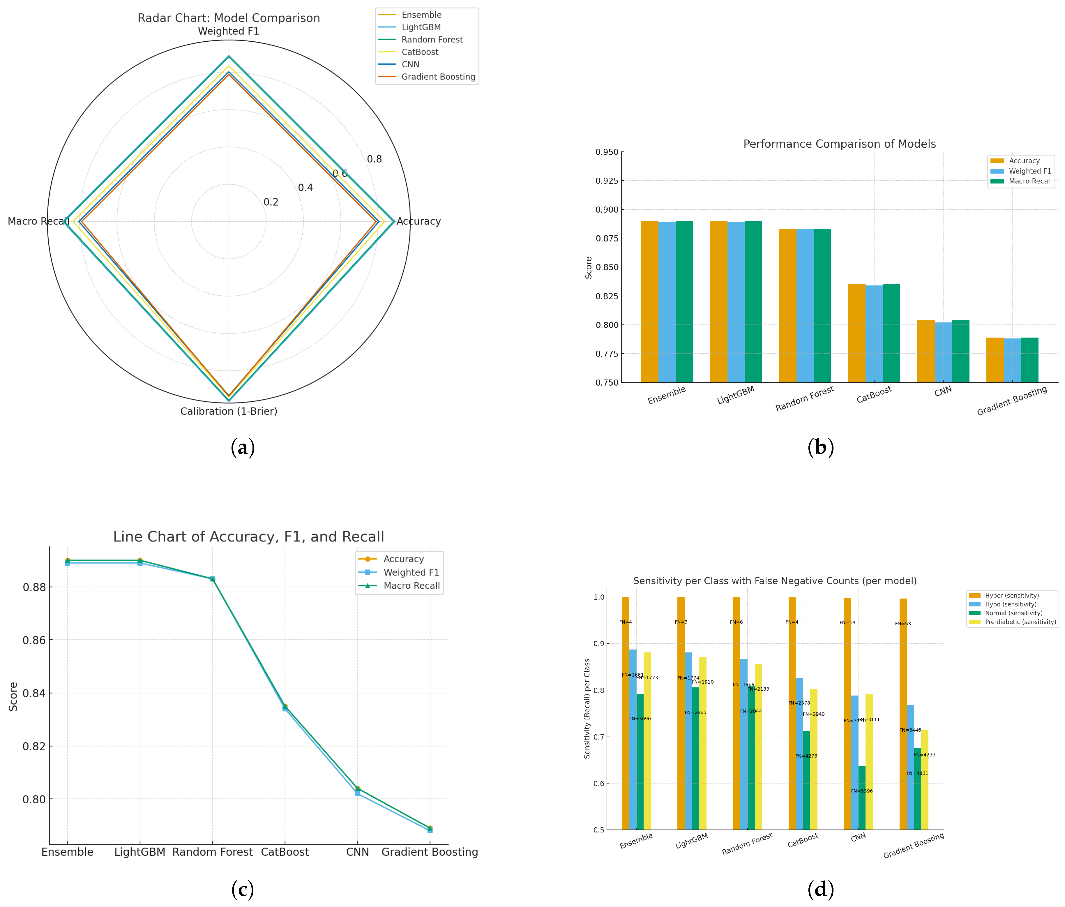
We’ve conducted a comparative assessment of six models looking at different aspects of performance. The radar and bar charts [(a) and (b)] indicate that the Ensemble and LightGBM modes achieve higher scores on Accuracy, Weighted F1, and Macro Recall (approximately 0.89) and highlight their evenness in the overall performance space (i.e., balanced performance). Random Forest scored comparably and CatBoost CNN and Gradient Boosting all scored lower than these top-performing models, especially in terms of macro recall indicating generalization ability (or lack thereof) across all classes of diabetes patients, especially at the macro-level level. The line chart also illustrates this outcome [(c)], in which the top three models have stable performance and there is a sharp drop for CNN and gradient-boosting, both of which show that ensemble-based models ours predictive framework are better at modeling structured physiological data than other models.

Similarly, the class-level analysis [(d)] give us an additional display of insights into sensitivity and false negative rates. All the models had nearly perfect recall for hyperglycaemia (>0.99). However, performance across normal and pre-diabetic classes dropped off scan appreciatively composed in accuracy the false negatives were higher. The Ensemble Model and LightGBM experienced the lowest misclassification rates across both of the minority classes, highlighting that these models are better at capturing nuanced signals that are important for being able to detect early onset of diabetes. Overall, the results highlight that following our analysis that ensemble learning based approaches are not only more reliable, but also more generalizable than CNN and boosting models. Therefore, they would be more appropriate for monitoring blood glucose without invasive techniques on subjects.

Figure 24. (a) Heatmap of Brier score per class across models, illustrating class-wise calibration performance; and (b) Heatmap of class-level metrics (accuracy, recall, and F1-score) across models.

Figure 24. (a) Heatmap of Brier score per class across models, illustrating class-wise calibration performance; and (b) Heatmap of class-level metrics (accuracy, recall, and F1-score) across models.

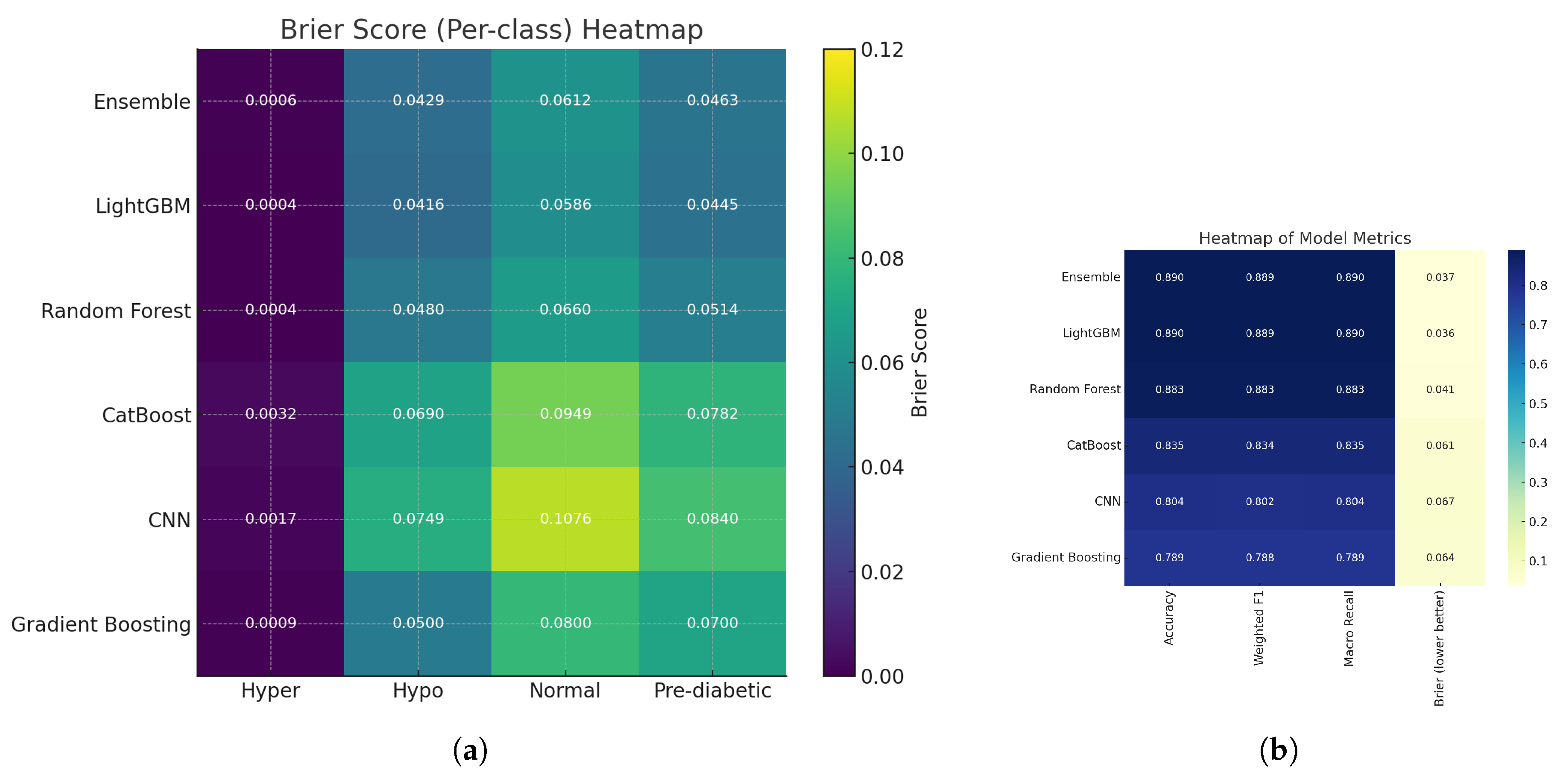
Using Brier score–based heatmaps, shown for class-wise and general evaluation, the calibration performance of the assessed models was further studied. The left heatmap displays normal, pre-diabetic, hyperglycemic, and hypoglycemic diabetes categories’ Brier scores. Lighter yellow shades suggest more calibration errors; hence, darker tones imply lower Brier values and so superior calibration. The yellow block shows that, for the normal class, the Convolutional Neural Network (CNN) had a fairly high mistake (Brier score ≈ 0.1076). This suggests that for this class the CNN’s forecast probability distribution deviated noticeably from the real results, which points to either an overconfident or underconfident probability projection.

Among the performance indicators displayed on the correct heatmap are accuracy, weighted F1 score, macro recall, and mean Brier score. Ensemble learning and LightGBM did With Brier scores of 0.037 and 0.036, CNN (0.067) and Gradient boosting are the best calibrated and predictive reliable together with high classification accuracy. Although it was quite accurate, Gradient Boosting (0.064) had worse calibration. The Brier score in the final column reveals how distinct classification accuracy and Probabilistic calibration. Although the Brier score, which gauges the reliability of predicted probabilities is defined as:

$$\mathrm{Brier}\mathrm{Score}={\displaystyle \frac{1}{N}}\sum _{i=1}^N{(p_i-y_i)}^2$$

where i ranges from 1 to N, N denotes the number of samples; $p_i$ denotes the predicted probability; $y_i$ denotes the actual binary outcome. A score of zero indicates perfect calibration; lower values suggest more reliable probability calculation. The exact binary result. Lower values mean more trustworthy forecast probabilities; a value of zero signals perfect calibration.

Overall results showed that ensemble-based models, and LightGBM model, which showed better classification accuracy, do a great job of calibrating probabilities to match actual class probabilities. This increased reliability makes them particularly useful in clinical decision support tools. On the other hand, models like CNN and Gradient Boosting still have some work to do, especially when it comes to accurately predicting normal glycemic states, to ensure their predicted probabilities are trustworthy.

5. Conclusions

This study focused on developing an artificial intelligence system for non-invasive blood glucose monitoring (NIBGM) using photoplethysmography (PPG) signals. The priority was to improve on the weaknesses of traditional invasive means of estimating glucose levels. The system classified the four diabetic states of hyperglycemia, hypoglycemia, pre-diabetes, and normoglycemia using advanced methods which included LightGBM, ensemble methods, gradient boosting, random forests, and neural networks. Ensemble and lightgbm model yielded the best outcomes with an accuracy of 89% and a weighted F1 score of 0.889, therefore, illustrating compelling proof for its possible clinical application.

Robustness and reliability were attained by an exhaustive validation framework consisting of ten-fold cross-validation, bootstrap resampling, subgroup sensitivity assessment against false negative instances, Brier scoring, and calibration by means of heatmap methods. These multi-layered statistical validations ensured the stability and the calibration-based performance of the models. Besides this preprocessing framework also employed AI-driven SMOTE balancing reducing class imbalance so as to enhance sensitivity for hypoglycemia detection. Feature selection was carried out systematically by means of L1 regularization, recursive elimination, cross-validation, and hyperparameter optimisation so as to reduce the feature set to twelve unique PPG-derived indices that covered morphological, temporal, statistical, as well as spectral categories.

In summary, this research demonstrates that artificial intelligence-driven models, coupled with intense validation as well as judiciously optimized feature selection, can significantly improve non-invasive glucose monitoring and provide reliable alternatives to conventional methods. Our proposed framework has important practical relevance for intelligent health care, in particular in regard to wearable devices intended for real-time diabetes management. Directions for future research include external validation on larger and more heterogeneous populations, integration with multimodal physiological signals, as well as development of adaptive personalized models towards broader clinical usefulness and long-lasting effects.

References

- Magliano, D.J.; Boyko, E.J.; committee, I.D.A.t.e.s. IDF DIABETES ATLAS; International Diabetes Federation: Brussels, 2021; pp. 1–141. [Google Scholar]
- Islam, T.T.; Ahmed, M.S.; Hassanuzzaman, M.; Amir, S.A.B.; Rahman, T. Blood Glucose Level Regression for Smartphone PPG Signals Using Machine Learning. Applied Sciences 2021, 11, 618. [Google Scholar] [CrossRef]
- Polak, A.G.; Klich, B.; Saganowski, S.; Prucnal, M.A.; Kazienko, P. Processing Photoplethysmograms Recorded by Smartwatches to Improve the Quality of Derived Pulse Rate Variability. Sensors 2022, 22. [Google Scholar] [CrossRef] [PubMed]
- Prabha, A.; Yadav, J.; Rani, A.; Singh, V. Intelligent estimation of blood glucose level using wristband PPG signal and physiological parameters. Biomedical Signal Processing and Control 2022, 78, 103876. [Google Scholar] [CrossRef]
- Zhang, J.; Zhang, Z.; Zhang, K.; Ge, X.; Sun, R.; Zhai, X. Early detection of type 2 diabetes risk: limitations of current diagnostic criteria. Frontiers in Endocrinology 2023, 14, 1260623. [Google Scholar] [CrossRef]
- Jancev, M.; Vissers, T.A.C.M.; Visseren, F.L.J.; van Bon, A.C.; Serné, E.H.; et al. Continuous glucose monitoring in adults with type 2 diabetes: a systematic review and meta-analysis. Diabetologia 2024, 67, 798–810. [Google Scholar] [CrossRef]
- Qawqzeh, Y.K.; Bajahzar, A.S.; Jemmali, M.; Otoom, M.M.; Thaljaoui, A. [Retracted] Classification of Diabetes Using Photoplethysmogram (PPG) Waveform Analysis: Logistic Regression Modeling. BioMed Research International 2020, 2020, 3764653. [Google Scholar] [CrossRef]
- Zeynali, M.; Alipour, K.; Tarvirdizadeh, B.; Ghamari, M. Non-invasive blood glucose monitoring using PPG signals with various deep learning models and implementation using TinyML. Scientific Reports 2025, 15, 1–23. [Google Scholar] [CrossRef]
- Elsayed, N.A.; Aleppo, G.; Aroda, V.R.; Bannuru, R.R.; Brown, F.M.; et al. 7. Diabetes Technology: Standards of Care in Diabetes—2023. Diabetes Care 2023, 46, S111–S127. [Google Scholar] [CrossRef]
- Martins, A.J.L.; Velásquez, R.J.; Gaillac, D.B.; Santos, V.N.; et al. A comprehensive review of non-invasive optical and microwave biosensors for glucose monitoring. Biosensors and Bioelectronics 2025, 271, 117081. [Google Scholar] [CrossRef]
- Moses, J.C.; Adibi, S.; Wickramasinghe, N.; Nguyen, L.; et al. Non-invasive blood glucose monitoring technology in diabetes management: review. mHealth 2024, 10. [Google Scholar] [CrossRef]
- Wu, J.; Liu, Y.; Yin, H.; Guo, M. A new generation of sensors for non-invasive blood glucose monitoring. American Journal of Translational Research 2023, 15, 3825. [Google Scholar] [PubMed]
- Adigüzel, G.; Şentürk, Ü.; Polat, K. Blood Glucose Level Estimation Using Photoplethysmography (PPG) Signals with Explainable Artificial Intelligence Techniques. Open Journal of Nano 2024, 9, 45–62. [Google Scholar] [CrossRef]
- Hammour, G.; Mandic, D.P. An In-Ear PPG-Based Blood Glucose Monitor: A Proof-of-Concept Study. Sensors 2023, 23, 3319. [Google Scholar] [CrossRef] [PubMed]
- Satter, S.; Turja, M.S.; Kwon, T.H.; Kim, K.D. EMD-Based Noninvasive Blood Glucose Estimation from PPG Signals Using Machine Learning Algorithms. Applied Sciences 2024, 14, 1406. [Google Scholar] [CrossRef]
- Alghlayini, S.; Al-Betar, M.A.; Atef, M. Enhancing Non-Invasive Blood Glucose Prediction from Photoplethysmography Signals via Heart Rate Variability-Based Features Selection Using Metaheuristic Algorithms. Algorithms 2025, 18, 95. [Google Scholar] [CrossRef]
- Salamea-Palacios, C.; Montalvo-López, M.; Orellana-Peralta, R.; Viñanzaca-Figueroa, J. Photoplethysmography Feature Extraction for Non-Invasive Glucose Estimation by Means of MFCC and Machine Learning Techniques. Biosensors 2025, 15. [Google Scholar] [CrossRef]
- Shi, B.; Dhaliwal, S.S.; Soo, M.; Chan, C.; Wong, J.; et al. Assessing Elevated Blood Glucose Levels Through Blood Glucose Evaluation and Monitoring Using Machine Learning and Wearable Photoplethysmography Sensors: Algorithm Development and Validation. JMIR AI 2023, 2, e48340. [Google Scholar] [CrossRef]
- Naresh, M.; Nagaraju, V.S.; Kollem, S.; Kumar, J.; Peddakrishna, S. Non-invasive glucose prediction and classification using NIR technology with machine learning. Heliyon 2024, 10, e28720. [Google Scholar] [CrossRef]
- Ali, M.; Li, J.; Fan, B.; Nie, Z. PPG Based Noninvasive Blood Glucose Monitoring Using Multi-View Attention and Cascaded BiLSTM Hierarchical Feature Fusion Approach. IEEE Journal of Biomedical and Health Informatics 2025, 29, 4692–4702. [Google Scholar] [CrossRef]
- Susana, E.; Ramli, K.; Murfi, H.; Apriantoro, N.H. Non-Invasive Classification of Blood Glucose Level for Early Detection Diabetes Based on Photoplethysmography Signal. Information 2022, 13, 59. [Google Scholar] [CrossRef]
- Hina, A.; Saadeh, W. Noninvasive Blood Glucose Monitoring Systems Using Near-Infrared Technology—A Review. Sensors 2022, 22, 4855. [Google Scholar] [CrossRef] [PubMed]
- Soliman, A.Y.; Nor, A.M.; Fratu, O.; Halunga, S.; Omer, O.A.; Mubark, A.S. Non-Invasive Glucose Level Monitoring from PPG using a Hybrid CNN-GRU Deep Learning Network. In Proceedings of the 2024 IEEE Conference on Advanced Topics on Measurement and Simulation (ATOMS 2024); 2024; pp. 299–302. [Google Scholar] [CrossRef]
- Chan, P.Z.; Jin, E.; Jansson, M.; Chew, H.S.J. AI-Based Noninvasive Blood Glucose Monitoring: Scoping Review. Journal of Medical Internet Research 2024, 26, e58892. [Google Scholar] [CrossRef] [PubMed]
- Chu, J.; Yang, W.T.; Lu, W.R.; Chang, Y.T.; Hsieh, T.H.; Yang, F.L. 90% Accuracy for Photoplethysmography-Based Non-Invasive Blood Glucose Prediction by Deep Learning with Cohort Arrangement and Quarterly Measured HbA1c. Sensors 2021, 21, 7815. [Google Scholar] [CrossRef]
- Li, T.; Wang, Q.; Lei, L.; An, Y.; Guo, L.; et al. Improvement of Non-Invasive Glucose Estimation Accuracy Through Multi-Wavelength PPG. IEEE Journal of Biomedical and Health Informatics 2025, 29. [Google Scholar] [CrossRef]
- Idris, N.F.; Ismail, M.A.; Jaya, M.I.M.; Ibrahim, A.O.; Abulfaraj, A.W.; Binzagr, F. Stacking with Recursive Feature Elimination-Isolation Forest for classification of diabetes mellitus. PLOS ONE 2024, 19, e0302595. [Google Scholar] [CrossRef]
- Afsaneh, E.; Sharifdini, A.; Ghazzaghi, H.; Ghobadi, M.Z. Recent applications of machine learning and deep learning models in the prediction, diagnosis, and management of diabetes: a comprehensive review. Diabetology and Metabolic Syndrome 2022, 14, 1–39. [Google Scholar] [CrossRef]
- Kaliappan, J.; Saravana Kumar, I.J.; Sundaravelan, S.; Anesh, T.; et al. Analyzing classification and feature selection strategies for diabetes prediction across diverse diabetes datasets. Frontiers in Artificial Intelligence 2024, 7, 1421751. [Google Scholar] [CrossRef]
- Parvez, A.; Mufti, M.J. Generalizable Diabetes Risk Stratification via Hybrid Machine Learning Models. https://arxiv.org/pdf/2509.20565, 2025.
- Casacchia, N.J.; Lenoir, K.M.; Rigdon, J.; Wells, B.J. Development, validation and recalibration of a prediction model for prediabetes: an EHR and NHANES-based study. BMC Medical Informatics and Decision Making 2024, 24, 387. [Google Scholar] [CrossRef]
- Hageh, C.A.; Henschel, A.; Zhou, H.; Zubelli, J.; Nader, M.; et al. Improving T2D machine learning-based prediction accuracy with SNPs and younger age. Computational and Structural Biotechnology Journal 2025, 27, 2772–2781. [Google Scholar] [CrossRef]
- Kornas, K.; Tait, C.; Negatu, E.; Rosella, L.C. External validation and application of the Diabetes Population Risk Tool (DPoRT) for prediction of type 2 diabetes onset in the US population. BMJ Open Diabetes Research & Care 2024, 12, 3905. [Google Scholar] [CrossRef]
- Templeman, E.L.; Ferrat, L.A.; Parikh, H.M.; You, L.; Triolo, T.M.; et al. Development and recalibration of a multivariable type 1 diabetes prediction model for type 1 diabetes across multiple screening studies. BMC Medicine 2025, 23, 433. [Google Scholar] [CrossRef]
- Zhang, T.; Huang, M.; Chen, L.; Xia, Y.; Min, W.; Jiang, S. Machine learning and statistical models to predict all-cause mortality in type 2 diabetes: Results from the UK Biobank study. Diabetes & Metabolic Syndrome: Clinical Research & Reviews 2024, 18, 103135. [Google Scholar] [CrossRef]
- Ma, Y.; Wang, Z.; Yao, Z.; Lu, B.; He, Y. Machine learning in the prediction of diabetic peripheral neuropathy: a systematic review. BMC Medical Informatics and Decision Making 2025, 25, 1–14. [Google Scholar] [CrossRef]
Disclaimer/Publisher’s Note: The statements, opinions and data contained in all publications are solely those of the individual author(s) and contributor(s) and not of MDPI and/or the editor(s). MDPI and/or the editor(s) disclaim responsibility for any injury to people or property resulting from any ideas, methods, instructions or products referred to in the content. |
© 2025 by the authors. Licensee MDPI, Basel, Switzerland. This article is an open access article distributed under the terms and conditions of the Creative Commons Attribution (CC BY) license (https://creativecommons.org/licenses/by/4.0/).
Copyright: This open access article is published under a Creative Commons CC BY 4.0 license, which permit the free download, distribution, and reuse, provided that the author and preprint are cited in any reuse.