
Submitted:
14 July 2023
Posted:
18 July 2023
You are already at the latest version
Abstract
Drilling operation is the major cost factor for the industry. Appropriately designed operations are essential for successful drilling. Optimized drilling operations also allow enhanced drilling performance and reduce the drilling cost. This is achieved by increasing the bit life (minimizing premature bit wear), drilling faster that allows reducing drilling time, and also reducing tripping operations. The paper presents two parts. The first part compares the parametric physic-based swab and surge simulation results obtained from Bingham Plastic, Power Law, and Robertson and Stiff models. The aim is to show how the model predictions deviate from each other. Two 80-20 Oil Water ratios (OWR) and two 90-10 OWR oil-based drilling fluids with 1.96 sg and 2.0 sg were considered in vertical- and deviated wells. Simulation results analysis revealed that the deviations depend on the drilling fluid’s physical and rheological parameters as well as the well trajectory. Moreover, the model’s predictions were inconsistent. Data-driven machine learning (ML) modeling makes up the second section. Data-driven modeling was done using both software-generated datasets and field datasets. Results show that the Random Forest Regressor (RF), Artificial Neural Network (ANN), Long Short-Term Memory (LSTM), LightGBM, XGboost, and Multivariate regression models predict the training and test datasets with higher R-squared and minimum root means square values. Deploying the ML model in real-time applications and the planning phase would have the potential application of artificial intelligence for well planning and optimization processes.
Keywords:
Swab
; Surge
; Simulation
; Machine Learning modeling
; Oil Based Drilling fluids
1. Introduction
Poorly designed drilling operations can make drilling less efficient. This can cause problems like damaged bits, slower drilling, twisted drill strings, and broken MWD tools. These issues can lead to unwanted round-tipping operations and drive up the cost of drilling. During tripping operations, the movement of the drill string in and out of the wellbore, making and breaking connections, results in undesired non-productive time and hence increases drilling costs. It is rational to draw out/run in the drill string to its permissible threshold speed and shorten the time connected with the tripping operation. However, the drill string movement beyond the allowable speed will lead to well collapse and fluid influx to the wellbore during tripping out (swabbing effect) and well fracturing while tripping in (surging effect). The consequence of well collapse struck the drill string, and in the worst case, the fate of the unstruck drill string/BHA is to shoot the drill string/BHA and perform an undesired sidetrack. This results in a significant increase in the well budget.
Similarly, well fracturing results in drilling fluid losses. Here, the problem also increases the operational and non-productive time, increasing the overall drilling budget. Predicting appropriate well pressure mitigates the possible well instability issues and kick influxes.
Over the years, researchers built models to predict the surge and swab effects based on different assumptions and conditions, such as steady-state and dynamic/transient. Burkhardt (1961) developed a model to estimate surge and swab pressures for Bingham Plastic fluids where the fluid flows steadily [1]. Schuh (1964) used a similar approach when developing a power-law fluid model, assuming steady-state flow in a concentric annulus [2]. Fontenot and Clark (1974) developed a model to predict the swab pressure for Bingham Plastic and Power Law fluids [3]. Mitchell (1988) produced a dynamic model, including several new factors, such as mud rheology, the elasticity of the pipe and the cement, formation, changing temperatures, and viscous forces [4]. Ahmed et al. (2008) showed experimentally the impact of pipe rotation on well pressure in the eccentric and concentric well filled with Xanthan Gum and Polyanionic Cellulose-based fluid [5]. Crespo et al. (2010) developed a simplified swab and surge model for yield power-law fluids [6]. Srivastav et al. (2012) experimentally showed that the speed of the trip, mud properties, annular clearance, and the eccentricity of the pipe affects the surge and swab pressures highly [7]. Gjerstad et al. (2013) employed Kalman Filter to predict and calibrate surge and swab pressures in real time for Herschel-Bulkely fluids based on differential pressure equations [8]. Ming et al. (2016) employed computational fluid dynamics techniques to build a swab and surge prediction model for concentric annuli. The comparison of simulations and experiments indicates an accuracy of up to 75% in predicting surge and swab pressures [9].
Fredy et al. (2012) utilized narrow slot geometry and regression techniques to develop a steady-state swab and surge prediction model and considered the compressibility of fluid, formation, and pipe elasticity [10]. Erge et al. (2015) build a numerical annular pressure loss estimation model for the eccentric annuli [11]. He at el. (2016) employs numerical simulations and regression techniques to forecast drilling operations' swabs and surge pressures. The model indicates ±3% maximum error compared to experimental measurements [12]. Evren M. et al. (2018) implied artificial neural network techniques and performed parametric studies on pressure loss [13]. Ettehadi et al. (2018) developed an analytical model for calculating pressure surges caused by drill string movement in Herschel Bulkley fluids [14]. Shwetank et al. (2020) developed a two-layer neural network to predict the swab and surge pressures [15]. Shwetank et al. (2020) also performed a parametric study to identify the impact of different parameters on the surge and swab pressures [16]. Zakarya et al. (2021) utilized numerical and Random Forest models to study the flow of drilling fluid through an eccentric annulus during tripping operations and the effect of eccentricity on the annular velocity and apparent viscosity profiles [17]. Amir et al. (2022) employed deep-learning techniques to predict the equivalent circulating mud density during tripping and drilling operations [18].
However, the reviewed scientific works show that the swab and surge models do not consider all the operational, fluid properties and well geometry setups. Therefore, the applicability of the swab surge models is valid for the considered assumptions and experimental setup conditions.
This study aimed to compare the predictions of swab and surge physics-based models, specifically the Bingham Plastic, Power Law, and Robertson and Stiff models.'.The evaluation was conducted in vertical and deviated wells, using four different types of drilling fluids. Additionally, two machine learning models were applied to demonstrate how data-driven models can predict the synthetic physics-based dataset created. We also implemented six of the Machine Learning (ML) models for the prediction of equivalent circulating mud density (ECD) on the actual field data acquired via a high-speed (wired drill pipe) telemetry system.
2. Swab Surge Modelling
2.1. Machine Learning Modeling
Figure 1 summarizes the modeling and performance evaluation process employed in this paper. The first step was field data pre-processing to clean and select features for ML modeling. The second step is ML modeling, performed by splitting 70% of the dataset for the model training and the rest 30% for the model testing. Seven ML algorithms are selected: Polynomial, Multivariate regression, LSTM, LightBGM, XGboost, Artificial Neural network, and Random forest. Finally, the model accuracy performance was also evaluated with a coefficient of determination (R2), standard deviation, mean square error, and root mean square.
2.1.1. Description of models
2.1.1.1. Multivariate Regression
For the field dataset, several features affect the ECD in the wellbore. Due to this reason, we used multivariable regression for multiple independent variables/features (x1, x2, x3… xn ) to predict the target variable y (ECD). The multiple linear regression model is the linear combination of the weighted features and is written as (Anderson,2003) [19].
2.1.1.2. Random Forest
Random forest regression is a Supervised Machine Learning Algorithm. The concept behind the Random forest algorithms is that it builds decision trees based on different inputs and takes their majority vote for classifying and averages in case of regression, Breiman (2001) [20]. Random forest reduces overfitting since it averages over the independent trees Han et al. (2011) [21]. In this paper, the Random Forest regression model was applied for both field and synthetic data.
2.1.1.3. Artificial Neural Network
The ANN model is built by using a feed-forward backpropagation network. The training algorithm used in this study was ReLu. In addition, the MSE loss function calculates the changing weight and updates the weight change and a new learning state. The network was built with three layers: an input, a hidden, and an output layer. For the synthetic data, the input layer consists of a single neuron (i.e., tripping speed (Vp), the hidden layers are three neurons, and the output layer has one neuron (i.e., ECD). Multiple input layers are (running speed, bit position) for field data, and the output layer is ECD. ANN model was also implemented for synthetic and field datasets.
2.1.1.4. LightGBM
LightGBM algorithm is a Python gradient-boosting decision tree framework. The gradient algorithm was selected for faster training data and higher efficiency. Moreover, it exhibits lower memory usage, improved accuracy, and the ability to handle large-scale data [22]. LightGBM algorithm employed to the field dataset.
2.1.1.5. XGBOOST
XGBoost is a family of gradient tree-boosting algorithms and an ensemble learning technique. The method was initially developed by (Chen et al. 2016) [23]. The gradient boosting combines several weak models to get a robust model. Decision trees are trained in a series of iterations using XGBoost weak models. After each iteration, the method updates the model with a new decision tree to fix the flaws in the prior trees. Each tree attempts to anticipate the residual of the proceeding trees as the trees are trained on those errors. One of the advantages of XGBoost is its capability to tackle missing data. It divides the data into the left and right branches at each decision tree node and automatically learns how to handle the missing values. [24] LightGBM algorithm employed for the field dataset.
2.1.1.6. LSTM
Long Short-Term Memory is formed of Recurrent Neural Network (RNN). It has a great capacity to capture the underlying correlations among the different features in the data (Chujie Tian et al. 2018) [25]. The most widely used LSTM is gradient-based backpropagation and has a faster learning rate in real-time implementation. [26] We used LSTM ML modeling for the field dataset.
2.2. Models Accuracy Evaluation
The model performance accuracy is evaluated with the commonly used statistical parameters such as root mean square error (RMSE), Mean square error (MSE), regression coefficient (R2), and Standard deviation(SD), Mongomery, 2019 [27].
Mean Square Error (MSE):
Root Mean Square Error (RMSE):
Regression Coefficient (R2):
Standard deviation (SD.):
2.3. Description of tripping out data
The dataset used in this study was obtained from a field located on the Norwegian shelf. The data is recorded by the multiple downhole sensors located at different positions along the wellbore, as shown in Figure 2. The pressure sensors mounted on the enhanced measurement systems (EMS) tool transfer the measured to the surface via a wired drill pipe bidirectional telemetry system that transmits data at 57000 bps (Reeves et al.) [28].
The Data While Tripping Tool (NOV DWT) was employed to assess the connectivity of the wired drill string throughout the tripping operations.DWT makes it possible to stay connected during the tripping operations, which was a long desire of E&P companies to collect the downhole pressure and temperature data [29].
The trip was made from 1060 m to 330 m in an 8.5" hole section. The sensors close to the bit are 67 m above the bit, 2nd sensor is 328 m, and 3rd sensor is located at 575 m. However, in this paper, data from only sensors closer to the bit has been used. As shown in Figure 3, the data consists of the downhole Equivalent Mud Weight (EMW), Bit position, and running speed (VP).
2.2. Physics-based modeling
We use commercial software (DrillBenchTM [30]) to evaluate the swab and surge behaviors in vertical and horizontal well profiles filled with different drilling fluids.
2.1. Simulation Setup
2.1.1. Pore and Fracture Gradient
Figure 4 shows the pore - and fracture pressure gradient window used for the swab and surge simulation. The experimental well is constructed with a 9 5/8" casing set at 4000m. For the swab and surge simulation study, the density of the drilling fluid is assumed to be at mid-way between the tripping-in and tripping-out limits, as shown in the figure. The fracture gradient for the surging limit is at the casing show, which is 2.06 sg, and the maximum pore pressure for the swabbing limit is 1.93 sg. For practical work, one needs to compute the collapse pressure gradient and compare it with the pore pressure to determine the swabbing limit. The collapse gradient was not calculated here since detailed information on the drilling formation was unavailable. Therefore, we assumed the swab limit was based on the reservoir pressure.
2.1.2. Well Construction and Trajectory
Figure 5 shows the 4800 m measured depth well construction design through which the swab and surge phenomenon is simulated. The well is deviated with a maximum inclination of 36 deg with different azimuths. The survey data was obtained from a well drilled in Bangladesh [31]. The seabed is 109 m below the drill sea level. The 21-inch riser is used to connect the surface with the seabed. A tapered drilling string that connects 5" at the top and 3 ½" at the bottom is used. DrillbenchTM software was used to construct the experimental well [30].
2.1.3. Fluid Models
The swab and surge simulations are based on the hydraulic model. The model requires defining PVT for density predictions and also rheological models. Including tripping speeds, the density and viscosity parameters adjusted for the given temperature and pressure are used to calculate the pressure loss during swab and surge operations.
2.1.3.1. Fluid PVT models
We used the empirical Glassø oil density model formulated based on North Sea oil for density calculation. For the water density model, we used Dodson and Standing empirical model.
2.1.3.2. Rheology models
Three rheological models are implemented in the DrillbenchTM software [30]. These are Bingham Plastic (BP), Power Law (PL), and Robertson & Stiff (RS) models for the evaluation of swab and surge simulation.
Bingham Plastic model (BP):
Bingham Plastic is a two-parameter rheology model. The model assumes a constant viscosity as the shear rate increases. The shear stress and shear rate vary linearly with the excess of the yield stress. The model reads [32,33]
where: PV is Plastic viscosity, Is the shear rate, and YS is the yield stress.
The plastic viscosity and yield stress values are calculated from the 600 and 300 rpm dial readings of the Fann viscometer as:
Power Law model (PL):
Unlike the Bingham Plastic model, the shear stress - the shear rate of the drilling fluid described by Power law is without yield stress, and the viscosity decreases as the shear rate increases. The model reads: [32,33].
Robertson-Stiff (RS):
Robertson – Stiff model is a three-parameter model. The model describes drilling fluids and cement slurries. The viscosity decreases as the shear rate increases. [34].
The shear rate, , can be calculated using the interpolation method, which is the corresponding value of . The shear stress, , is the geometric mean between the maximum and the minimum given as:
2.1.4. Drilling Fluids
Figure 6 and Figure 7 are the four Oil-based drilling fluids (OBM) with different oil-water ratios (OWR). The fluids were used in the experimental well to assess the Swab and Surge models prediction. To fit the well stability issue window shown in Figure 4, the density of the drilling fluids was elevated to 1.96 sg and 2.0 sg while keeping the measured viscometer data. The fluids are filled in the vertical and the deviated experimental well. The 2.0 sg mud weight is about 0.06 sg and 0.07 sg away from the midline's lower (swab limit) and upper (surge limit). On the other hand, to simulate near overpressure, the mud weight is reduced to 1.96 sg, which is about 0.03 sg and 0.13 sg away from the lower and the upper limit.
The rheological parameters derived from the measurement and the rheology models are used as input for calculating the swab and surge hydraulics models. The three rheological models (Eq. 6, 9, and 12) are used to quantify the rheological parameters of the drilling fluids presented in Figure 6 and Figure 7. Here, the rheological modeling is based on curve fitting between the model and the measured viscometer dataset. The model prediction was evaluated by the absolute mean error percentile between the model calculated and the measurement as: [37]
Table 1 and Table 2 are the rheological parameters and the percentile error derivation for the 80-20 and 90-10 of the drilling fluids shown in Figure 6. Results show that the Robertson and Stiff model records a lower error deviation. This indicates the model describes the drilling fluids better than the Power law and the Bingham plastic models.
Similarly, Table 3 and Table 4 show the rheological parameters and the percentile error deviation of the fluids system displayed in Figure 7. Again, the Robertson and Stiff model exhibited a lower error deviation.
However, the lower error deviation for the rheological model prediction does not mean that the hydraulic model accurately predicts the well pressure; Jeyhun (2014) has shown this. [38].
3. Results
3.1. Physics-based simulation results
3.1.1. Result 1
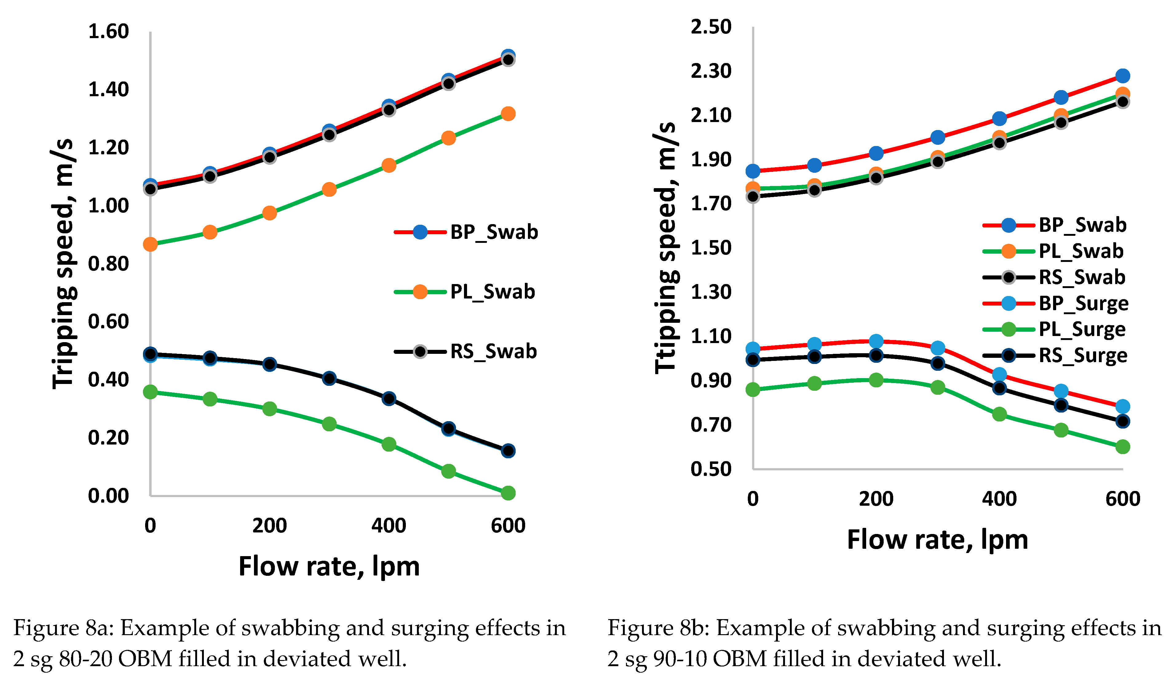
The first computer swab and surge experiments were conducted by using the drilling fluids shown in Figure 6. The simulations have been performed at different tripping speeds while circulating. Figure 8a and Figure 8b show the critical allowable swab and surge tripping speeds that lead to the lower limit (i.e., at 1.93 sg) and the upper limit at the casing shoe (i.e., 2.06 sg), respectively. The examples presented are obtained from the results in deviated well filled with 2.0 sg 80-20 and 90-10 OBMs. The comparison shows that the model prediction varies in the different fluid types. For instance, in the well filled with 80-20 OBM, the swabbing pressures obtained from Robertson, Stiff, and Bingham plastic are almost equal, but the Power law model underpredicts. For the 90-10 OBM, the Power Law and the Roberson swab speed predictions are closer, but the Bigham Plastic deviates from the two models. On the other hand, surge speeds show different behaviors. Another observation is that the 80-20 OBM surging pressure decreases as the flow rate increases. In contrast, the three models in the 90-10 OMB show an increase in surging pressure when the flow rate increases up to 300lpm and then decreases as the flow rate increases. The simulation results reveal that one cannot conclude which hydraulic model to trust when designing the swab and surge model unless they are compared with measurement.
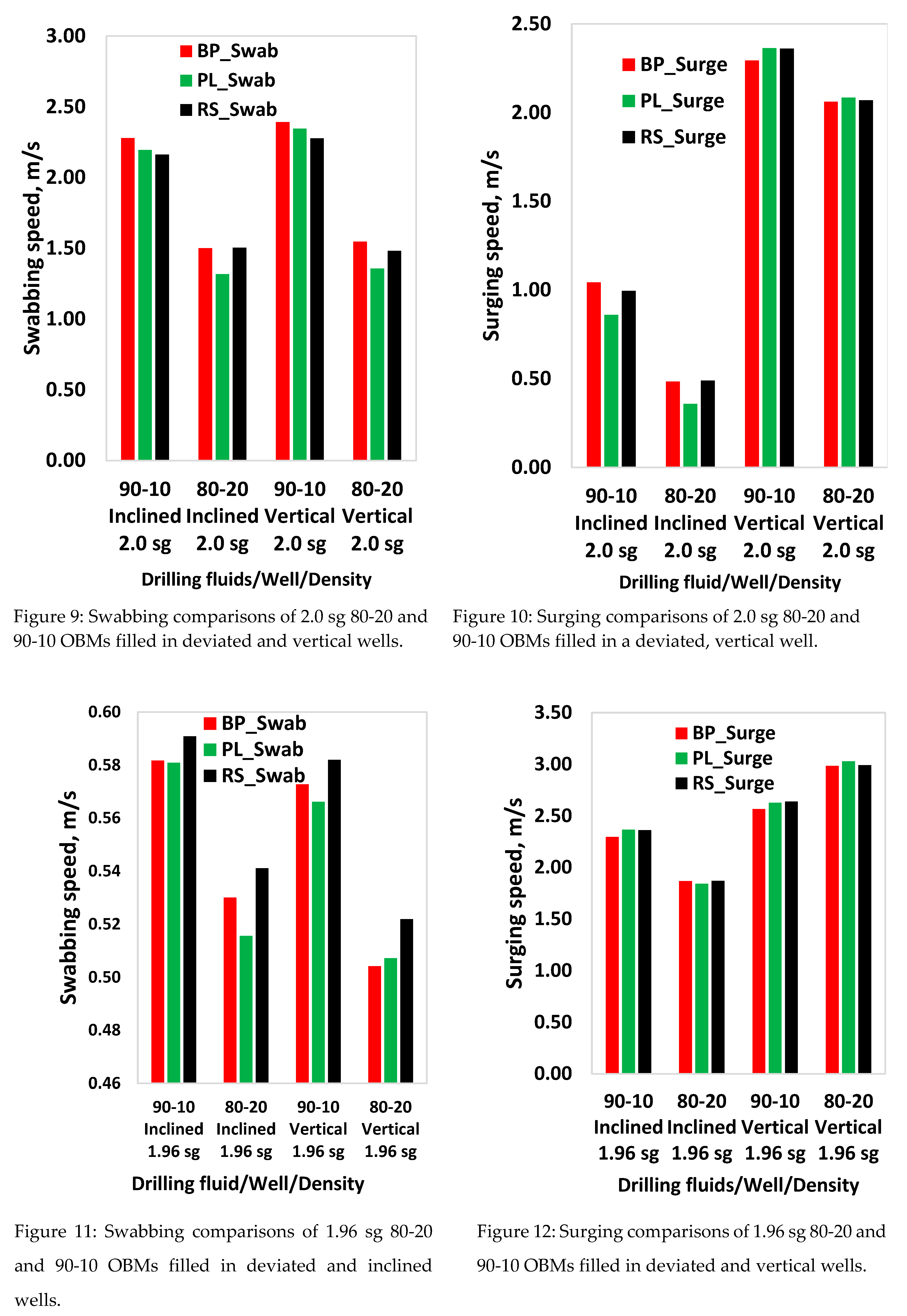
The simulation results also showed that the swabbing speed is higher during circulation, and the surging speed is higher when there is no circulation. To reduce the tripping time, it is important to trip out while in circulation and trip in while de-activating the rig pump. For further model performance evaluation, the swabbing speed was selected when the circulation flow rate was 600 liter per minute (lpm), and the surging speed was selected without the flow rate. The results are presented in Figure 9, Figure 10, Figure 11 and Figure 12. Results show the swabbing speed in the deviated and vertical wells filled with the two different drilling fluids.
Analysis
The percentile deviations of the BP from PL and RS models’ predictions are calculated for better quantification. The comparisons are presented in Table 5 and Table 6. As shown in Table 5, in vertical and deviated wells filled with the 2 sg 80-20 OBM drilling fluid, the BP’s swabbing speed model prediction is about 13.1 % and 12.4% higher than the PL model, respectively. On the other hand, for the 2.0 sg 90-10 OBM in the inclined and vertical wells, the BP model's prediction is about 5.1% and 4.8% higher than the RS, respectively. In the inclined well filled with 2 sg 90-10 and 80-20 OBMs, the surging speed model's prediction deviates from the PL by 17.6% and 25.9%, respectively. Table 6 shows the results obtained from the 1.96 sg drilling fluids. As shown, for both fluid types and wells, the BP deviation from the PL and RS records lower values.
3.1.2. Result 2
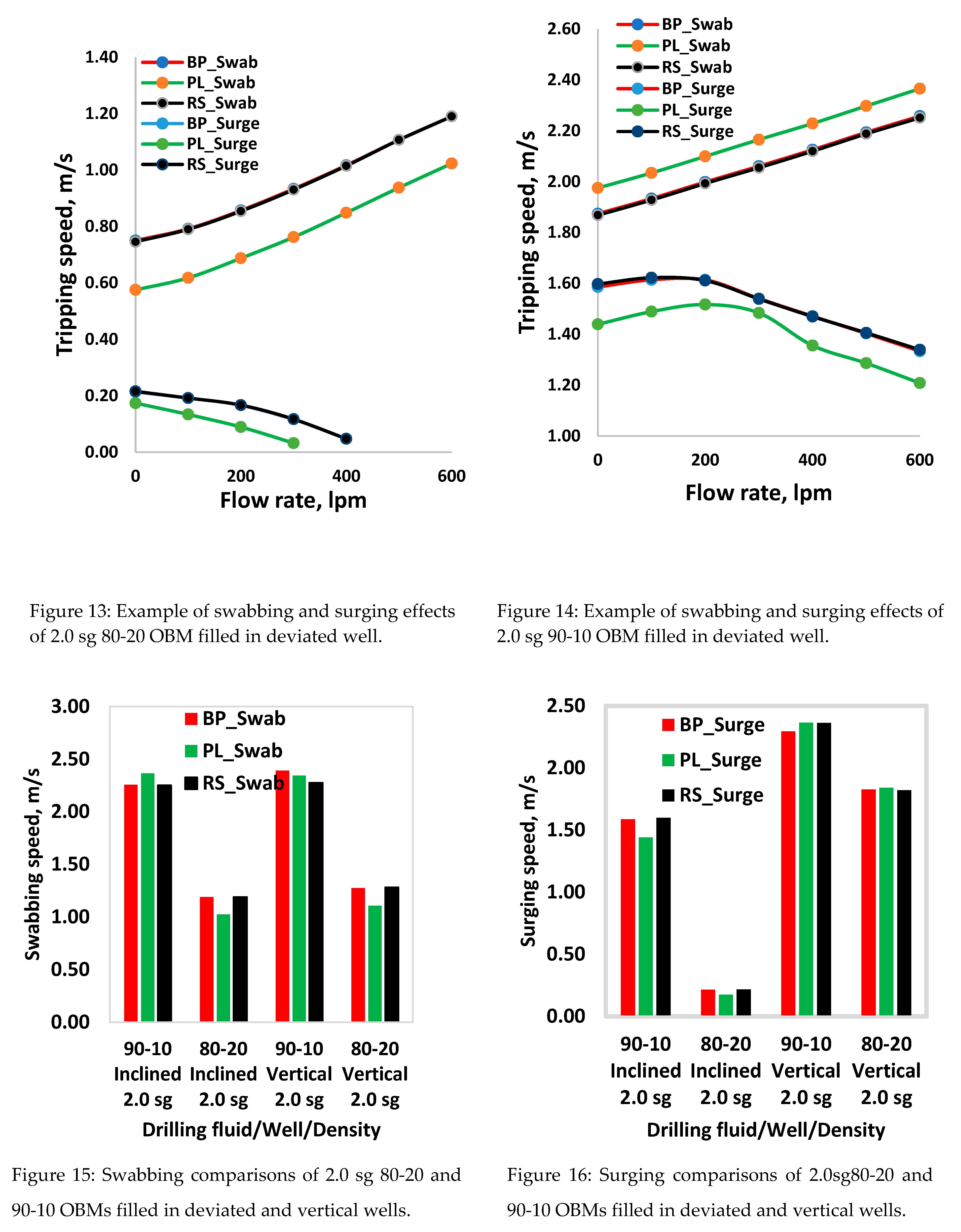
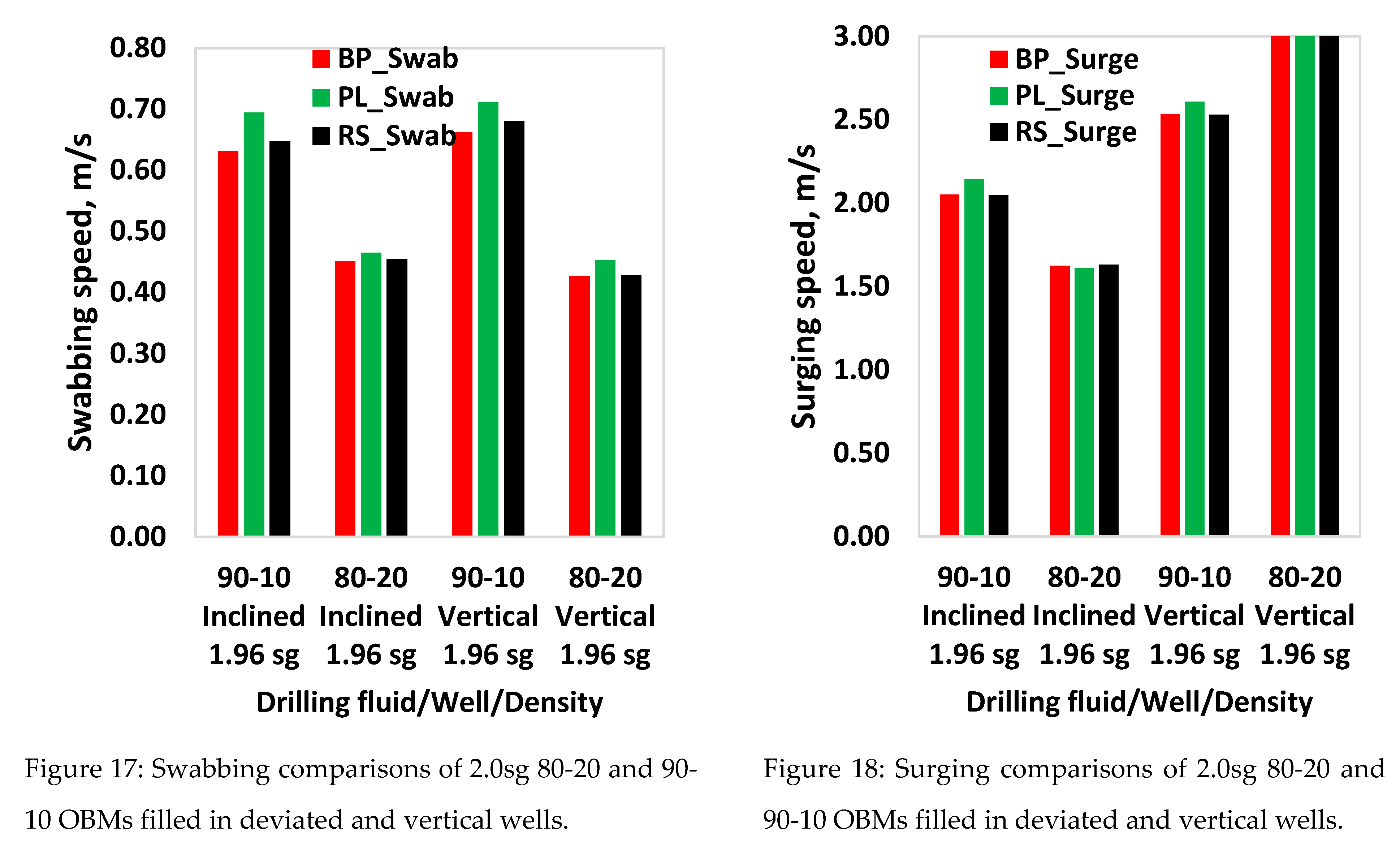
The second computer simulation results are based on the drilling fluids shown in Figure 7. The examples displayed in Figure 13 and Figure 14 are for the 80-20 -and 90-10 OBMs filled in a deviated well. The 80-20 OBM results show that BP and RS swabbing and surging speed prediction are nearly equal and differ from the Power law model for both fluids systems. However, the deviation of the Power law for swabbing is not consistent. Another observation here also that for the 90-10 OBM, the surging speed for the flow rate increments up to 300-400 lpm exhibited unexpected increases. For analysis purposes, the swabbing speeds (at 600 lpm) and surging speeds (no circulation) were considered, and the results are displayed in Figure 15, Figure 16, Figure 17 and Figure 18.
Analysis
Similarly, the percentile deviations of the swabbing and surging speed predicted by the PL and RS models (i.e., Figure 15, Figure 16, Figure 17 and Figure 18) are compared with the BP model. The comparisons are provided in Table 7 and Table 8. In the deviated well filled with the 2.0 sg 80-20 and 90-10 OBM, results showed that the swab and surge speeds prediction of the BP and RS is quite similar, recording less than 0.7% deviation. However, in the 80-20 OBM filled well, the BP model's swab and surge percentile deviation from PL records were 14% and 18.8%, respectively. Similarly, results obtained from the 90-10 OBM fluid show -4.8% and 9.3% deviations, respectively. Table 8 also shows the results obtained from the 1.96 sg drilling fluids (80-20 and 90-10 OBM) filled in the vertical and the inclined well. Results here also show that the deviation of the BP from the RS is relatively lower than from the PL model.
3.2. Machine Learning-based modeling result.
3.2.1. Result 1-Simulated and Laboratory-based data model.
The first ML modeling was performed by using the physics-based simulated dataset. The example presented here illustrates how the ML models predict the software-generated dataset. For this, the drilling fluid shown in Figure 7 was circulated in the experimental well.
Figure 19 shows the simulated synthetic dataset obtained from the BP and RS models. Simulation stopped at the maximum allowable tripping speed that causes the well pressure reaches to the weak point (i.e., at casing shoe, 2.06 sg). Figure 20 also shows the laboratory scale surge pressure gradient as a function of tripping speed [6].
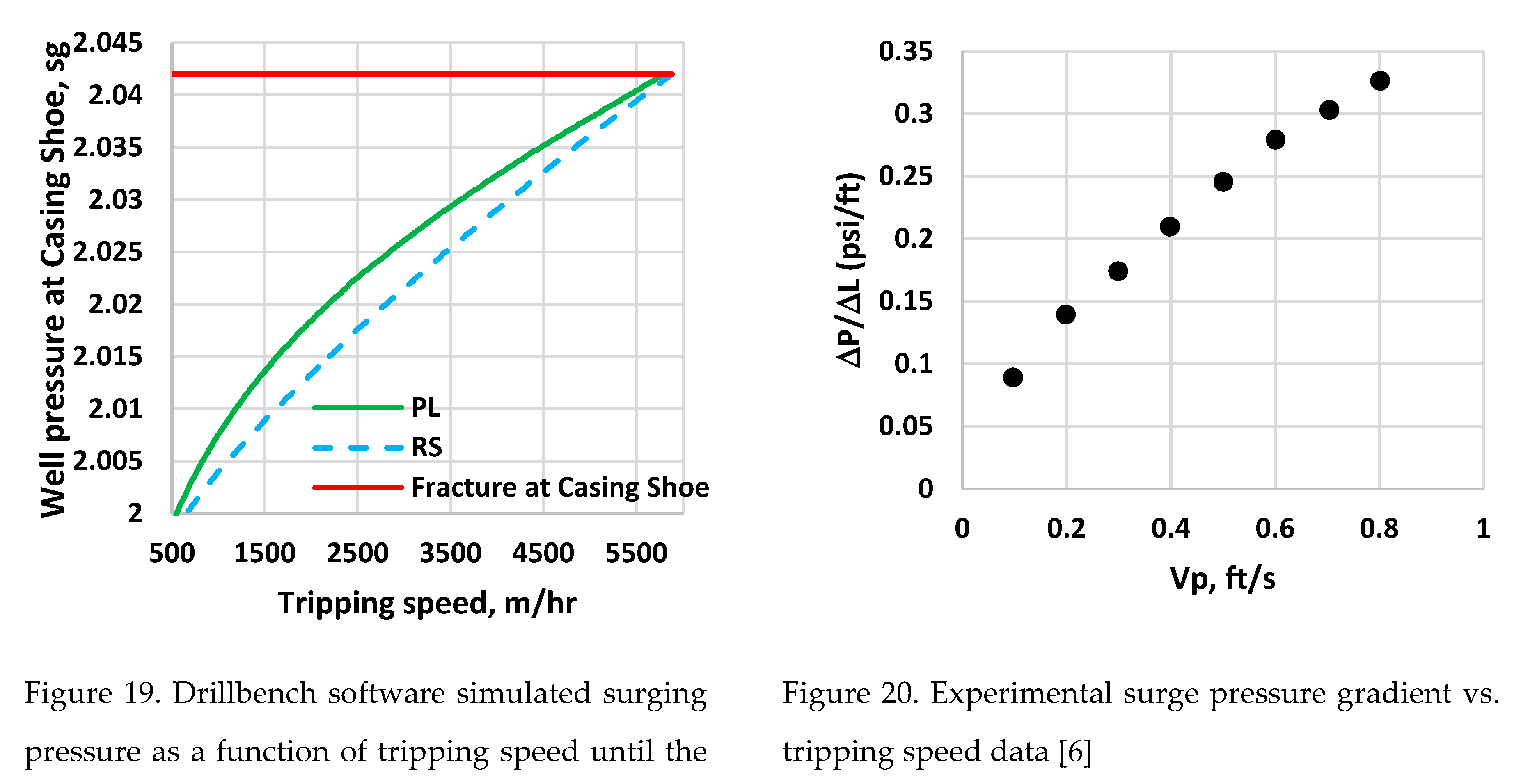
Polynomial inversion
The frictional pressure loss is proportional to the square of fluid flow. Similarly, the simulated (Figure 19) and the laboratory experimental (Figure 20) surge pressure variations with the pipe movement trend look like a second-order polynomial function. Therefore, the simulated and the experimental test data will be modeled as a polynomial function that includes both constant and middle terms. The maximum allowable well pressure is when the well pressure reaches the casing pressure (Pc). The variation of well pressure due to tripping speeds is given as follows:
where βο, β1 and β2 the curve fitting parameters will be determined from the green or blue dataset
Based on the knowledge of the case shoe pressure, one can therefore write well pressure at the critical tripping speed by inversion of Eq. 16 and given as:
Using the synthetic and experimental data, polynomial-based modeling was performed to estimate the curve fitting parameters (βο, β1, β2), and the results are provided in Table 9. Both models show higher R2 correlation values. However, it is essential to note that the polynomial-based modeling is applied only for the swab and surge field data or laboratory data if the pressure variation behaves as a polynomial when the tripping speed varies.
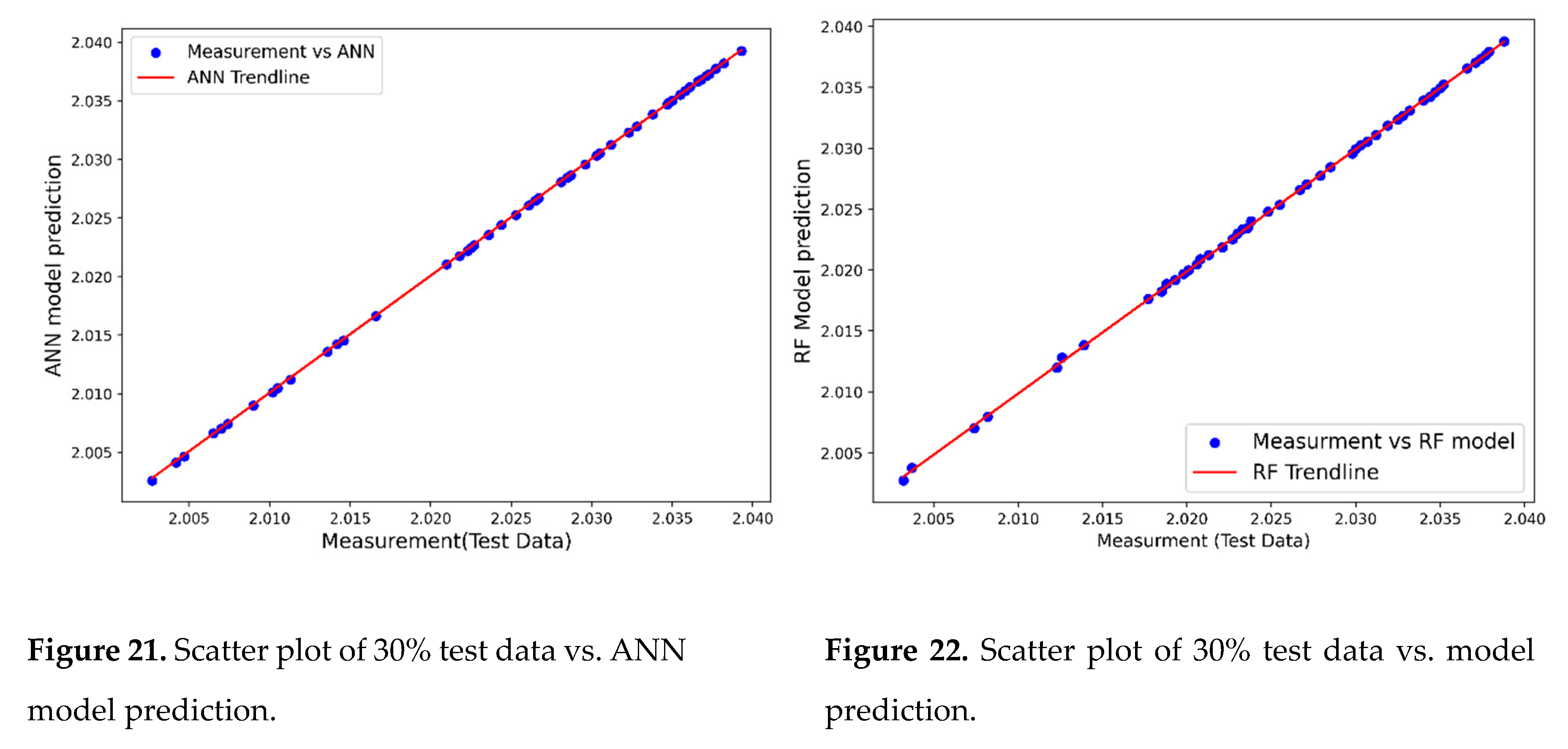
In the following, two Machine learning algorithms (ANN and RF) were selected to evaluate how the Data-driven-based modeling predicts the synthetic, simulated data shown in Figure 19.
ANN Modeling and Testing
Figure 21 compares the simulated dataset and ANN model predictions. Table 10 summarizes the ANN model performance analysis. As shown in the Table, the ANN model strongly correlated with the training and testing data with R2 values of 0.999 and 0.999, respectively. Moreover, the other statistical parameters also show that the model predicts the synthetic dataset perfectly. Since the physics model generates data without including noises, the ML model prediction shows the trustworthiness of the method.
RF Modeling and Testing
Similarly, Figure 22 shows the result obtained from the simulated dataset and RF model prediction. Table 10 also provides the RF model accuracy performance analysis. The R2 values of the training and testing datasets showed a strong correlation with 0.999 and 0.999, respectively. The statistical parameters also indicate that the RF method accurately predicts the simulated data.
3.2.2. Result 2-Field Data-Based Machine Learning
In Section §3.2.1, the selected RF and ANN methods significantly recovered the physics-based synthetic dataset. In this section, the application of six ML models will be tested on field-measured data, presented in Figure 3. Since the dataset contains noises, the data pre-processing was performed before ML modeling.
The ML-based model predicted, and the actual measured values are used for statistical accuracy analysis. For this, a linear regression model is derived based on the model predicted and the actual values. Figure 23, Figure 24, Figure 25, Figure 26, Figure 27 and Figure 28 show the ML model prediction and ML model linear trendline given as:
where, a and b are the slope and the intercept, respectively.
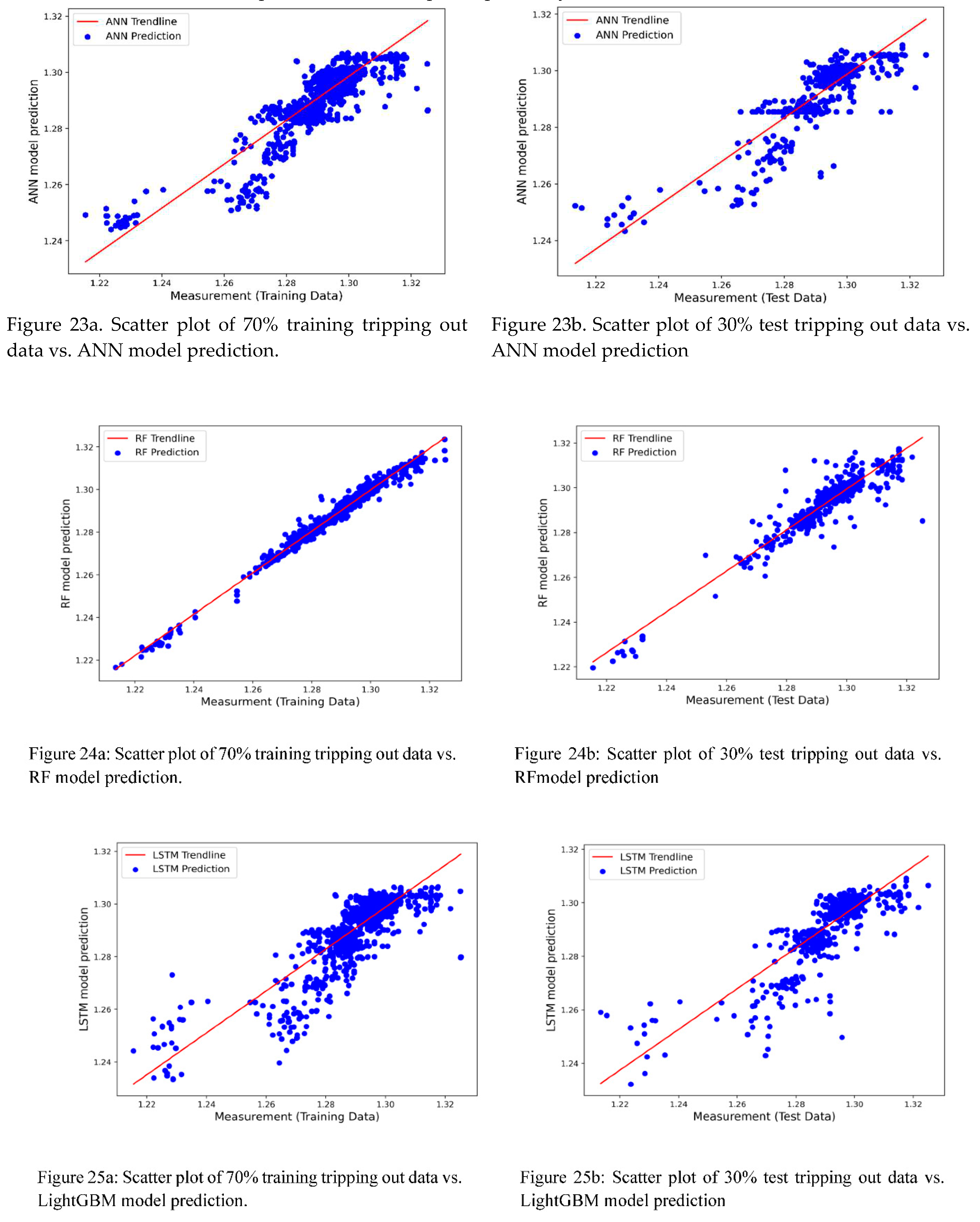
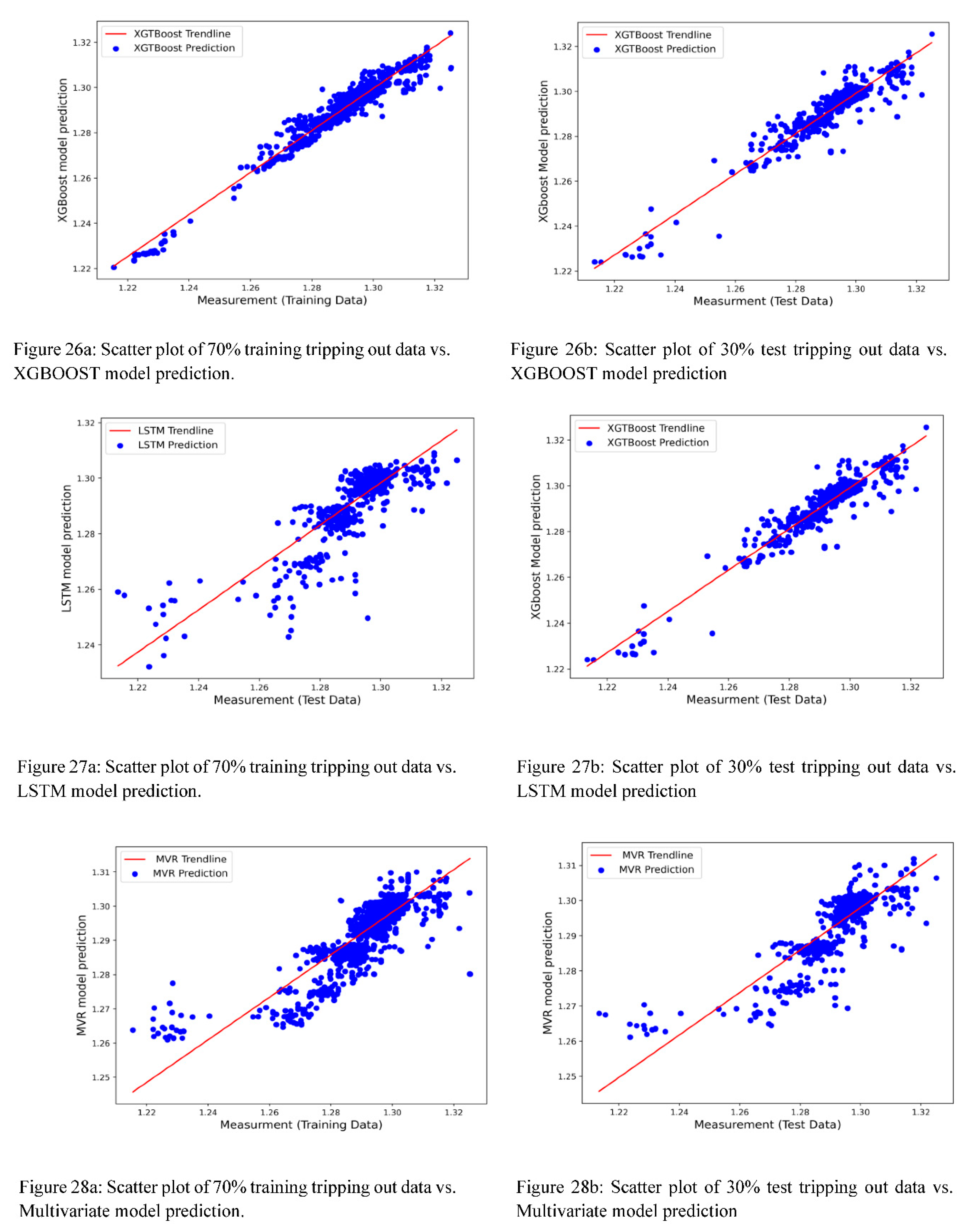
Table 11 shows the ML model's accuracy performance of the training and test results displayed in Figure 23, Figure 24, Figure 25, Figure 26, Figure 27 and Figure 28. The model's predictions exhibited a high R2 score, minimum mean square, and standard deviation. Results show the potential application of Machine learning modeling for the swab and surge field dataset.
4. Discussion
The tripping operation is lowering or withdrawing the drill string into the hole. The literature indicates that about 18% of the time is spent in tripping operations and is considered non-productive Christopher Jeffery et al. (2020) [29]. Tripping is performed, among others, to replace worn-out drill bits. Tripping string at a lower speed is safe concerning wellbore instability; however, it will increase the non-productive time and cost. Tripping at the higher speed will minimize the non-productive time, but pulling the strings over the optimum values will create undesired surging and swabbing pressures that lead to wellbore fracture and collapse/kick, respectively. For safe and efficient operation, it is imperative to predict the appropriate swab surge pressure precisely associated with the optimized tripping speeds.
Amir et al. (2022) [39] presented an extensive literature survey on surge/swab pressure models, which are developed based on physical laws (analytical models) and based experimental works (empirical models). The analytical models developed are based on several presumptions and the laboratory-controlled experimental setup condition. On the other hand, it is difficult to precisely quantify the degree of drill string eccentricity, wellbore roughness, sizes, and fluid properties in actual drilling well operation. Hence, the model prediction with uncertain input will not be correct. Moreover, the model predictions are also varying. This indicates the uncertainty of the parametric-based modeling for swab and surge models.
In this paper, first, we have conducted a physis-based swab and surge simulation study to evaluate the model prediction in different well trajectories filled with different rheological and physical properties of drilling fluids. The models are Bingham Plastic, Power Law, and Robertson and Stiff. Considered for the simulations were four oil-based drilling fluids with various viscosities, as well as vertical and deviated well profiles.
Observations based on the considered drilling fluids and experimental setup showed that:
- The model's predictions are inconsistent compared with each other.
- As the flow rates increase to about 200-300lpm, the surging speeds in a deviated well filled with 90-10 OBM show an increasing trend. Whereas, in 80-20 OMB, the surging speed shows a decreasing trend. On the other hand, in both fluids system, the surging speeds decrease when the flow rate increase above 300lpm. Even though the surge speeds trend of the three models' predictions seems similar, the values are quite different.
- Regarding rheology fluid description, the RS model has shown a lower error deviation. However, the Swab and Surge percentile deviation from the BP is lower than the RS with PL. The swab and surge predictions with the three models vary in the different well trajectories filled with different densities and viscosities.
- It is difficult to conclude the accuracy of the hydraulics model prediction based on how the model accurately describes the fluid rheological properties.
Generally, a model that considers all the physical processes and fluid properties is unavailable. It is, therefore, vital to calibrate models with a real-time measured dataset that considers the bulk effects in the wellbore on the dataset.
North Sea field-measured hydraulics data and the hydraulic model were compared by Lohne et al. in 2008 [40]. The comparison results revealed a difference between the measured and modeled values. This comparison demonstrates that the model is unable to predict the measurement. The model's parameters, including density, friction factor, and well path, are all ambiguous. The authors incorporated a calibration factor and set the friction factor value to only one because the model does not fully represent the physics. The authors created a dynamic calibration factor based on the collected data to calibrate the annulus and drill string pressure. Jeyhun (2014) [38] deployed five hydraulic models on both the laboratory and field data in a separate study and discovered that the predictions made from these models were inconsistent. For instance, the Herschel Bulkley model may forecast the hydraulics of fluid A in a pipe or annulus, whereas, for fluid type B, the Robertson and Stiff models work better than the others. This suggests that no universal solution anticipates the fluid's hydraulics in the wellbore owing to the fluid flow and pipe movements in and out of the well.
For the hydraulics model calibration, the accuracy of the measurement is also a critical factor. For this, the high-speed telemetry system WDP plays a significant role both in terms of a higher rate of data transmission with less noise Lohne et al. in (2008) [40], Reeves et al. (2006) [28], Christopher et al. (2020) [29]). Moreover, unlike Measurement-While-Drilling (MWD) sensors, the WDP telemetry allows a continuous measure of the downhole pressure with low or zero drilling fluid flow rate conditions, Michael (2003) [41]. The argument for data-driven-based modeling is that the measured data includes all possible factors contributing to the swab and surge impact. Wired pipe technology provides high-quality and fast data transfer. Moreover, knowing which physics-based modeling perfectly predicts the swab surge model as consistently and accurately as possible is difficult.
Therefore, the applicability of the selected ML models (ANN and RF) was first employed on the generated physics-based generated synthetic data. Results show that the ML perfectly discovered the dataset.
The performance of the six ML algorithms implemented on WPD tripping out field datasets has shown excellent prediction on both the training and test datasets.
5. Conclusion
Optimized swab and surge operations contribute to the reduction of tripping time and hence reduce non-productive time. This paper evaluates the physics-based swab and surge simulation and data-driven-based machine learning modeling of field surging field datasets.
The summary of the analysis shows that:
- The deviation of the swab surge model prediction from each model is inconsistent.
- Physics-based models generally require model calibration based on the accurate measured data.
- The reviewed physics models do not consider all operational parameters, constraints, fluid properties, and non-uniform eccentricity. Moreover, it is difficult to quantify these parameters precisely in drilling well.
- Data-driven-based modeling predicts both the training and unseen test data with higher accuracy.
The application of ML models on the swabbing pressure example presented in this paper indicates the potential of deploying an intelligent solution as online or offline-based modeling. This will allow drilling engineers to do drilling optimization and better well planning.
Author Contributions
A.M. Conceptualization, Methodology, Data processing, Software simulation, ML modeling, Testing, Result Analysis, Interpretation, and Writing. M.B.Methodology, Original draft preparation, Review and Editing. R.D. Supervision, Project administration, Funding acquisition, Review, and Editing. All authors have read and agreed to the published version of the manuscript.
Funding
This research was financed by the research council of Norway.
Institutional Review Board Statement
Not applicable.
Informed Consent Statement
Not applicable.
Data Availability Statement
Not applicable.
Acknowledgments
We thank Schlumberger for Drillbench free software to conduct Swab / Surge Simulation.
Conflicts of Interest
The authors declare no conflict of interest.
References
- Burkhardt, J. A. Wellbore pressure surges produced by pipe movement. Journal of petroleum technology 1961, 13, 595–605. [Google Scholar] [CrossRef]
- Schuh, F. J. Computer makes surge-pressure calculations useful. Oil and Gas Journal 1964, 31, 96. [Google Scholar]
- Fontenot, J.E.; Clark, R. An Improved Method for Calculating Swab and Surge Pressures and Circulating Pressures in a Drilling Well. Soc. Pet. Eng. J. 1974, 14, 451–462. [Google Scholar] [CrossRef]
- Mitchell, R.F. Dynamic Surge/Swab Pressure Predictions. SPE Drill. Eng. 1988, 3, 325–333. [Google Scholar] [CrossRef]
- Ahmed, Ramadan, and Stefan Miska. "Experimental study and modeling of yield power-law fluid flow in annuli with drill pipe rotation." IADC/SPE Drilling Conference. 2008.
- Crespo, F., Ahmed, R., Saasen, A., 2010. Surge and swab pressure predictions for yield-power-law drilling fluids, paper SPE-138938, Presented at the SPE Latin American & Caribbean Petroleum Engineering Conference, 1–3 December, Lima, Peru.
- Srivastav, R., Ramadan Ahmed, and Arild Saasen. Experimental Study and Modeling of Surge and Swab Pressures in Horizontal and Inclined Wells. AADE-17-NTCE-075 Technical Conference and Exhibition held at the Hilton Houston North Hotel, Houston, Texas, April 11-12, 2017. 11 April.
- Gjerstad, K., Time, R. W., Bjorkevoll, K. S. 2013. A Medium-Order Flow Model for Dynamic Pressure Surges in Tripping Operations. Society of Petroleum Engineers. [CrossRef]
- Tang, M.; Ahmed, R.; Srivastav, R.; He, S. Simplified surge pressure model for yield power law fluid in eccentric annuli. J. Pet. Sci. Eng. 2016, 145, 346–356. [Google Scholar] [CrossRef]
- Freddy Crespo, Ramadan Ahmed, Majed Enfis, Arild Saasen; and Mahmood Amani, "Surge-and-Swab Pressure Predictions for Yield-Power-Law Drilling Fluids" December 2012 SPE Drilling & Completion27.04 (2012): 574-585. 20 December.
- Erge, O.; Ozbayoglu, E.M.; Miska, S.Z.; Yu, M.; Takach, N.; Saasen, A.; May, R. The Effects of Drillstring-Eccentricity, -Rotation, and -Buckling Configurations on Annular Frictional Pressure Losses While Circulating Yield-Power-Law Fluids. SPE Drill. Complet. 2015, 30, 257–271. [Google Scholar] [CrossRef]
- He, S.; Tang, M.; Xiong, J.; Wang, W. A numerical model to predict surge and swab pressures for yield power law fluid in concentric annuli with open-ended pipe. J. Pet. Sci. Eng. 2016, 145, 464–472. [Google Scholar] [CrossRef]
- Ozbayoglu, E.M.; Oney, E.; Murat, A. O. Predicting the pressure losses while the drill string is buckled and rotating using artificial intelligence methods. Journal of Natural Gas Science and Engineering 2018, 56, 72–80. [Google Scholar] [CrossRef]
- Ettehadi, A.; Altun, G. Functional and practical analytical pressure surges model through herschel bulkley fluids. J. Pet. Sci. Eng. 2018, 171, 748–759. [Google Scholar] [CrossRef]
- Shwetank Krishna, Syahrir Ridha, and Pandian Vasant. "Prediction of Bottom-Hole Pressure Differential During Tripping Operations Using Artificial Neural Networks (ANN) " Intelligent Computing and Innovation on Data Science Proceedings of ICTIDS 2019 Lecture Notes in Networks and Systems Volume 118 2020 Springer Singapore, p. 379-388.
- Krishna, S.; Ridha, S.; Vasant, P.; Ilyas, S.U.; Irawan, S.; Gholami, R. Explicit flow velocity modelling of yield power-law fluid in concentric annulus to predict surge and swab pressure gradient for petroleum drilling applications. J. Pet. Sci. Eng. 2020, 195, 107743. [Google Scholar] [CrossRef]
- Belimane, Z.; Hadjadj, A.; Ferroudji, H.; Rahman, M.A.; Qureshi, M.F. Modeling surge pressures during tripping operations in eccentric annuli. J. Nat. Gas Sci. Eng. 2021, 96, 104233. [Google Scholar] [CrossRef]
- Mohammad, A., Karunakaran, S., Panchalingam, M., & Davidrajuh, R. (2022, December). "Prediction of Downhole Pressure while Tripping". In 2022 14th International Conference on Computational Intelligence and Communication Networks (CICN) (pp. 505-512). IEEE.
- Anderson TW. "An Introduction to Multivariate Statistical Analysis". 3rd Edition, ISBN: 978-0-471-36091-9 July 2003 Available from An Introduction to Multivariate Statistical Analysis, 3rd Edition | Wiley.
- Breiman L. (2001). "Random forests. Machine learning". 45(1), 5-32. Available from randomforest2001.pdf. Available online: berkeley.edu.
- Han J, Kamber M, Jian PJ. "Data Mining: Concepts and Techniques. " 3rd Edition - June 9, 2011 eBook ISBN: 9780123814807 available from Data Mining. Concepts and Techniques, 3rd Edition (The Morgan Kaufmann Series in Data Management Systems). Available online: sabanciuniv.edu.
- Ke, G., Meng, Q., Finley, T., Wang, T., Chen, W., Ma, W., & Liu, T. Y. (2017). "Lightgbm: A highly efficient gradient boosting decision tree". Advances in neural information processing systems, 30 (2017).
- Chen, Tianqi, and Carlos Guestrin. "Xgboost: A scalable tree boosting system." Proceedings of the 22nd acm sigkdd international conference on knowledge discovery and data mining. 2016.
- Chen, Tianqi, and Carlos Guestrin. "Xgboost: Reliable large-scale tree boosting system." Proceedings of the 22nd SIGKDD Conference on Knowledge Discovery and Data Mining, San Francisco, CA, USA. 2015.
- Tian, C.; Ma, J.; Zhang, C.; Zhan, P. A Deep Neural Network Model for Short-Term Load Forecast Based on Long Short-Term Memory Network and Convolutional Neural Network. Energies 2018, 11, 3493. [Google Scholar] [CrossRef]
- Sepp Hochreiter and Jürgen Schmidhuber. "Long Short-Term Memory."In: Neural Comput. 9.8 (Nov. 1997), pp. 1735–1780. ISSN: 0899-7667.
- Douglas CM. "Introduction to Statistical Quality Control".8th Edition; ISBN: 978-1-119-39930-8 August 2019 available from Introduction to Statistical Quality Control, 8th Edition | Wiley.
- Reeves, Michael, J. Macpherson, Ralf Zaeper, D. Bert, Jerry Shursen, K. Armagost, D. Pixton, and Maximo Hernandez. "High-Speed Drillstring Telemetry Network Enables New Real-Time Drilling and Measurement Technologies." In SPE/IADC Drilling Conference and Exhibition, pp. SPE-99134. SPE, 2006.
- Christopher Jeffery; Stephen Pink; Jennifer Taylor; Richard Hewlett. "Data While Tripping DWT: Keeping the Light on Downhole" SPE-202398-MS Paper presented at the SPE Asia Pacific Oil & Gas Conference and Exhibition, Virtual, November 2020.
- Drillbench Dynamic Drilling Simulation Software. Available online: slb.com.
- Tanmoy Chakraborty. 2012 "Performing simulation study on drill string mechanics, Torque, and Drag. " MSc Thesis University of Stavanger, 2012.
- Recommended Practice on the Rheology and Hydraulics of Oil-Well Drilling Fluids, API RP 13D Fourth Edition. American Petroleum Institute, (June 1995).
- Bourgoyne, A.T., Chenevert, M.E., Millheim, K.K. and Young, F.S. "Applied Drilling Engineering" SPE, Richardson, Texas (1991) 2.
- Robertson, R.E.; Stiff, H.A., Jr. An Improved Mathematical Model for Relating Shear Stress to Shear Rate in Drilling Fluids and Cement Slurries. Soc. Pet. Eng. J. 1976, 16, 31–36. [Google Scholar] [CrossRef]
- Sharman, Thomas. "Characterization and performance study of OBM at various oil-water ratios". MSthesis. University of Stavanger, Norway, 2015.
- Strømø, Simen Moe. "Formulation of New Drilling Fluids and Characterization in HPHT". MSthesis. University of Stavanger, Norway, 2019.
- Ochoa, Marilyn Viloria. "Analysis of drilling fluid rheology and tool joint effect to reduce errors in hydraulics calculations". Texas A&M University, 2006.
- Sadigov, J.; Mesfin, B. Analyses of Field Measured Data With Rheology and Hydraulics Models. International Journal of Fluids Engineering 2016, 8, 1–12. [Google Scholar]
- Mohammad, A.; Davidrajuh, R. Modeling of Swab and Surge Pressures: A Survey. Appl. Sci. 2022, 12, 3526. [Google Scholar] [CrossRef]
- Lohne, H. P., Gravdal, J. E., Dvergsnes, E. W., Nygaard, G., & Vefring, E. H. (2008, December). "Automatic calibration of real-time computer models in intelligent drilling control systems-results from a north sea field trial". In IPTC 2008: International Petroleum Technology Conference (pp. cp-148). European Association of Geoscientists & Engineers.
- Jellison, M. J., Hall, D. R., Howard, D. C., Hall Jr, H. T., Long, R. C., Chandler, R. B., & Pixton, D. S. (2003, February). "Telemetry drill pipe: enabling technology for the downhole internet". In SPE/IADC Drilling Conference and Exhibition (pp. SPE-79885).
Figure 1.
Summary of ML modeling and Performance analysis.
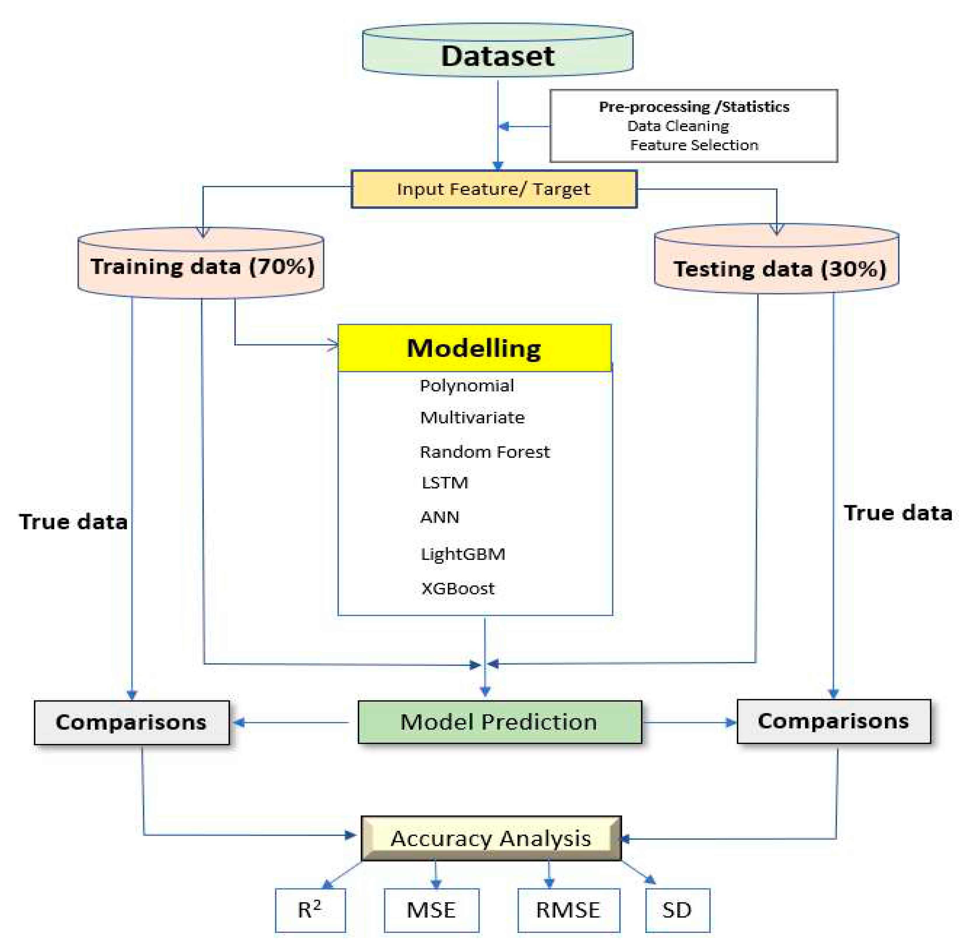
Figure 2.
Sensors placement along the wellbore.
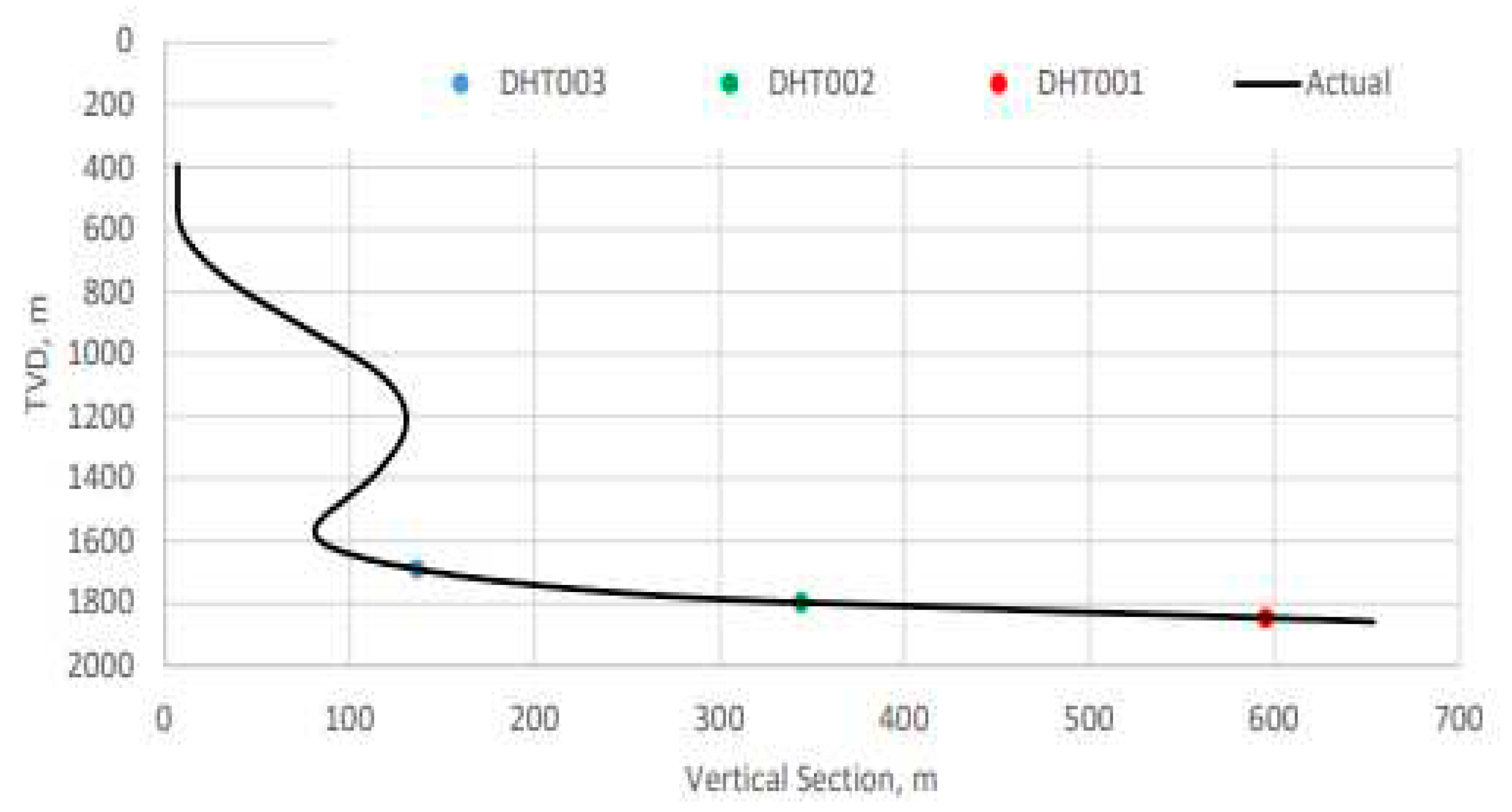
Figure 3.
Trip out dataset.
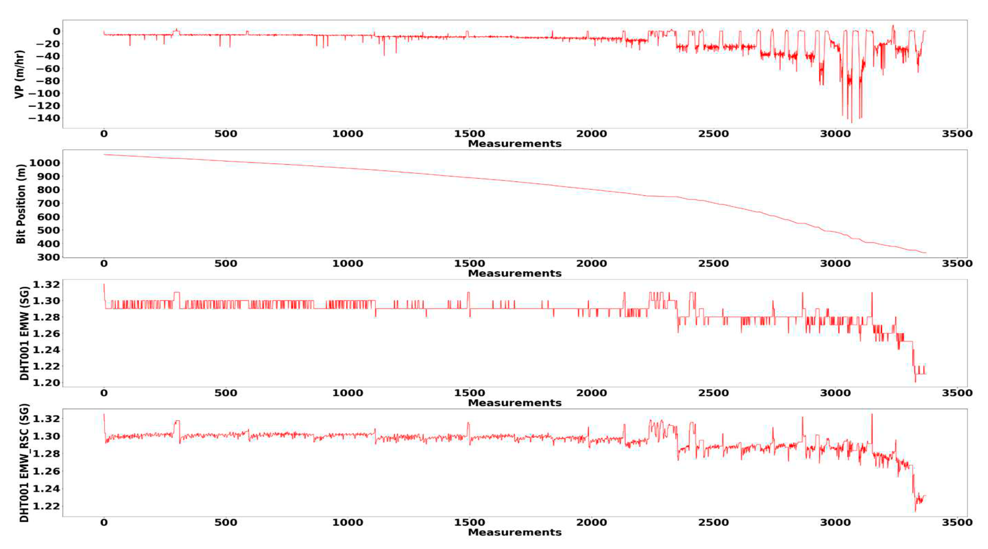
Figure 4.
Pore Pressure and Formation Strength Prognosis.
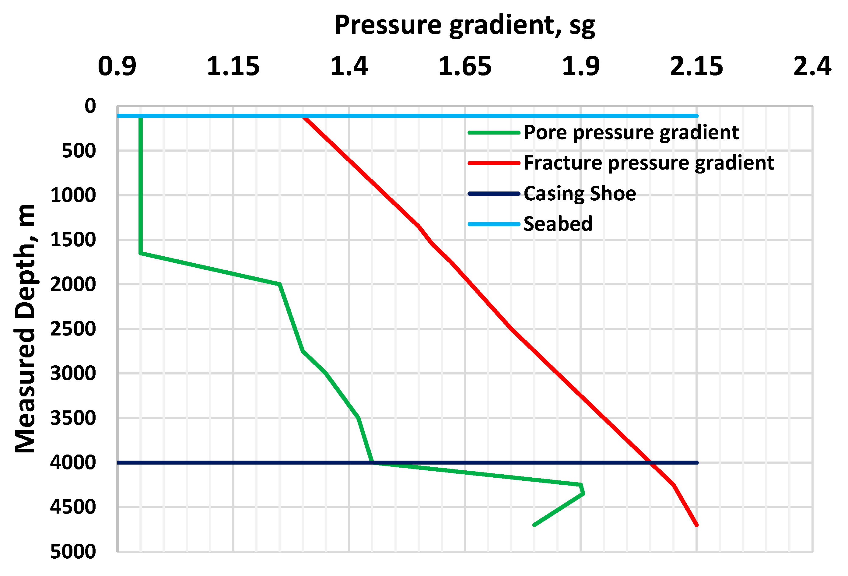
Figure 5.
Experimental well structure and well trajectory.
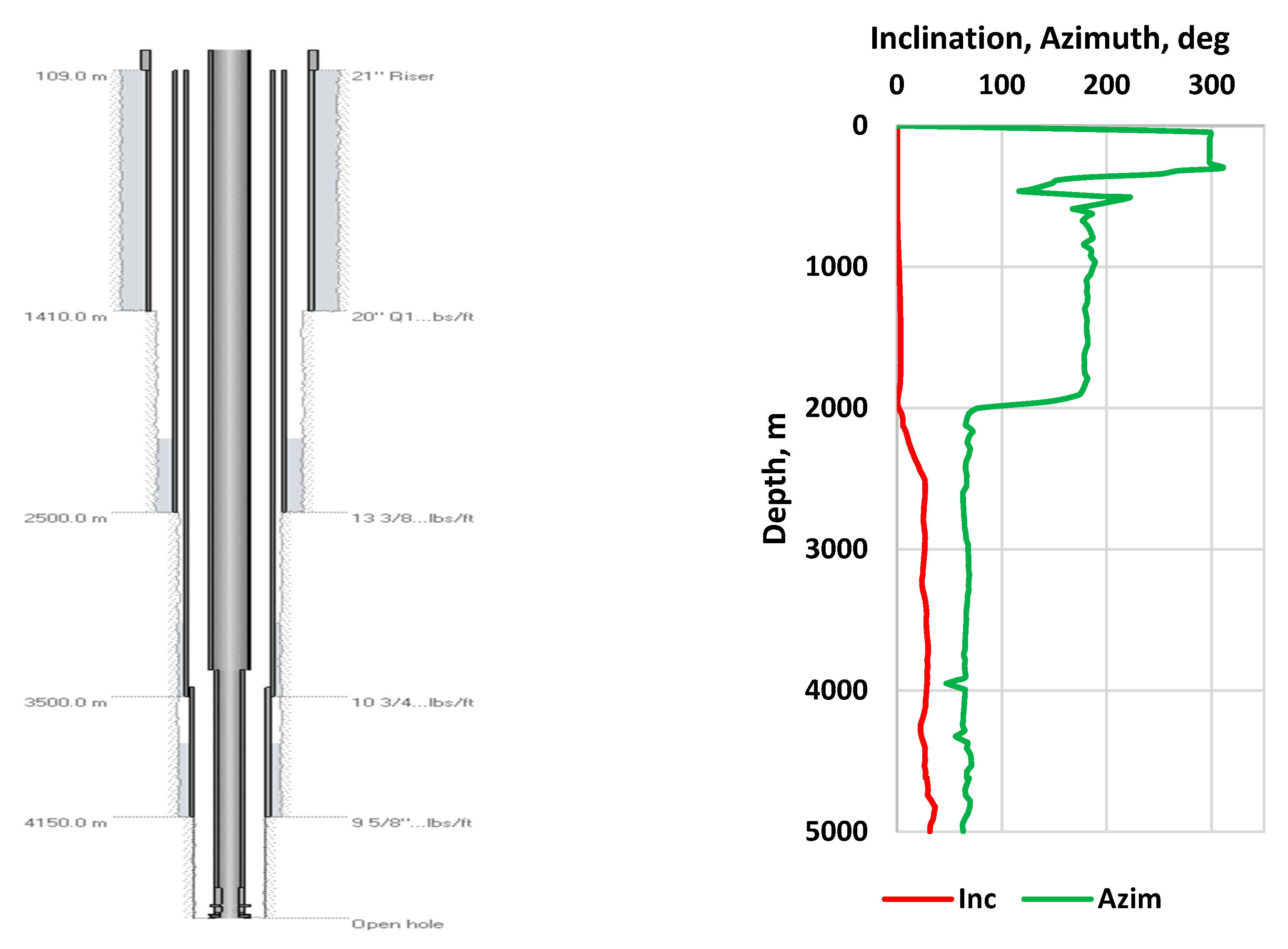
Figure 6.
80/20 and 90/10 OBM viscometer data measured at 20 0C [35].
Figure 6.
80/20 and 90/10 OBM viscometer data measured at 20 0C [35].
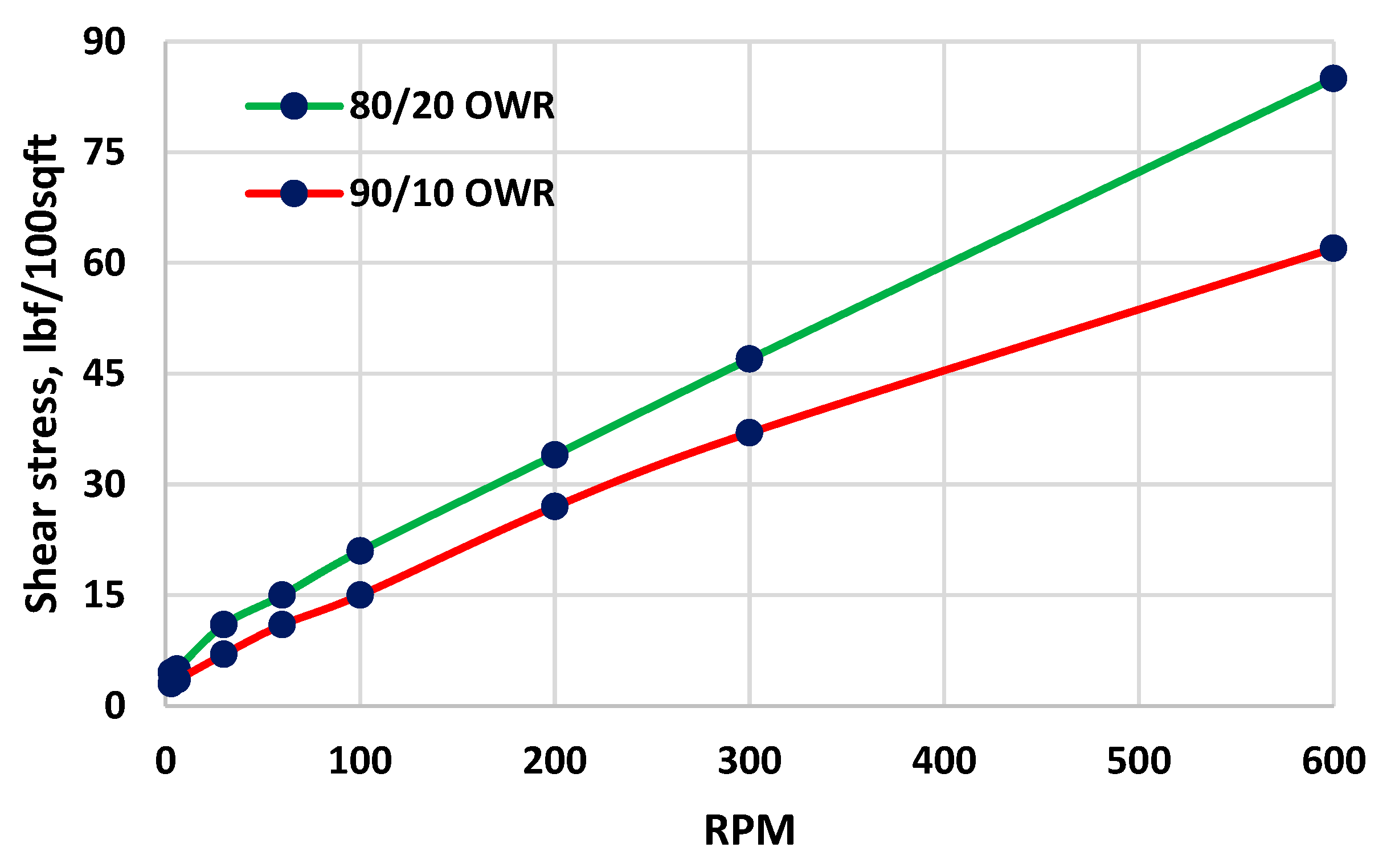
Figure 7.
80/20 and 90/10 OBM viscometer data measured at 20 0C [36].
Figure 7.
80/20 and 90/10 OBM viscometer data measured at 20 0C [36].
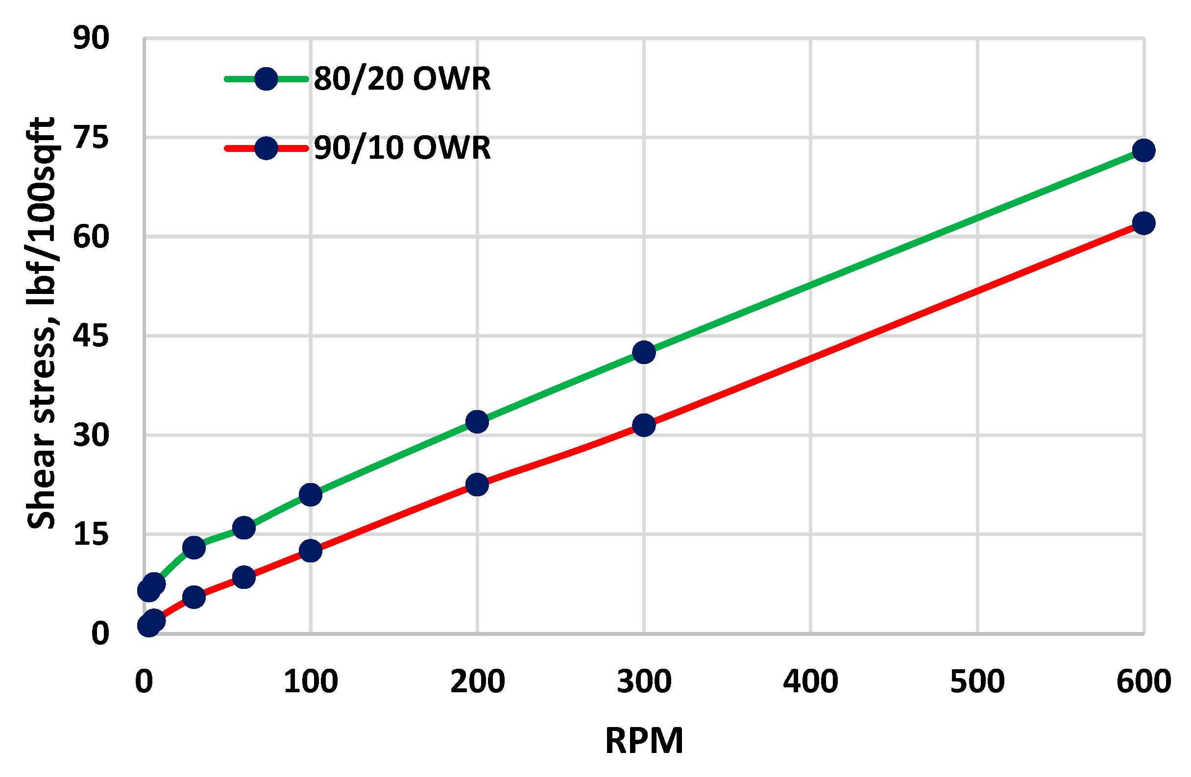

Table 1.
Figure 6's 80-20 OMB rheological parameters.
Table 1.
Figure 6's 80-20 OMB rheological parameters.
| Rheology Models | Parameters | % Error | |
|---|---|---|---|
| Bingham Plastic (BP) | YS [lbf/100sqft] | 6.0613 | 13.2 |
| PV [cP] | 40.314 | ||
| Power law (PL) | n [-] | 0.5461 | 13.6 |
| k [lbfsn/100sqft] | 1.6560 | ||
| Robertson and Stiff (RS) | A[lbfsn/100sqft] | 0.2618 | 1.5 |
| B [-] | 0.8384 | ||
| C [s-1] | 26.670 | ||
Table 2.
Figure 6's 90-10 OBM rheological parameters.
Table 2.
Figure 6's 90-10 OBM rheological parameters.
| Rheology Models | Parameters | % Error | |
|---|---|---|---|
| Bingham Plastic (BP) | YS [lbf/100sqft] | 4.8431 | 21.9 |
| PV [cP] | 29.820 | ||
| Power law (PL) | n [-] | 0.5704 | 12.2 |
| k [lbfsn/100sqft] | 1.0800 | ||
| Robertson and Stiff (RS) | A[lbfsn/100sqft] | 0.1792 | 2.1 |
| B [-] | 0.8551 | ||
| C [s-1] | 24.418 | ||
Table 3.
Figure 7's 80-20 OMB rheological parameters.
Table 3.
Figure 7's 80-20 OMB rheological parameters.
| Rheology Models | Parameters | % Error | |
|---|---|---|---|
| Bingham Plastic (BP) | YS [lbf/100sqft] | 8.69 | 11.1 |
| PV [cP] | 33.13 | ||
| Power law (PL) | n [] | 0.435 | 12.2 |
| k [lbfsn/100sqft] | 3.005 | ||
| Robertson and Stiff (RS) | A[lbfsn/100sqft] | 0.404 | 2.3 |
| B [-] | 0.751 | ||
| C [s-1] | 40.48 | ||
Table 4.
Figure 7's 90-10 OBM rheological parameters.
Table 4.
Figure 7's 90-10 OBM rheological parameters.
| Rheology Models | Parameters | % Error | |
|---|---|---|---|
| Bingham Plastic (BP) | YS [lbf/100sqft] | 1.724 | 13.6 |
| PV [cP] | 30.26 | ||
| Power law (PL) | n [] | 0.720 | 7.7 |
| k [lbfsn/100sqft] | 0.384 | ||
| Robertson and Stiff (RS) | A[lbfsn/100sqft] | 0.138 | 5.6 |
| B [-] | 0.884 | ||
| C [s-1] | 8.890 | ||
Table 5.
Comparisons of Figure 9 and Figure 10 (80-20 and 90-10 OBMs) with 2.0 sg density in vertical and inclined wells.
Table 5.
Comparisons of Figure 9 and Figure 10 (80-20 and 90-10 OBMs) with 2.0 sg density in vertical and inclined wells.
| OBM/ Well/Density | Swabbing | Surging | |||
|---|---|---|---|---|---|
| % BP to PL change | % BP to RS change | % BP to PLchange | % BP to RSchange | ||
| 90-10 Inclined 2.0 sg | 3.63 | 5.12 | 17.58 | 4.66 | |
| 80-20 Inclined 2.0 sg | 13.11 | 0.82 | 25.86 | -1.15 | |
| 90-10 Vertical 2.0 sg | 1.97 | 4.82 | -3.06 | -2.97 | |
| 80-20 Vertical 2.0 sg | 12.39 | 0.72 | -1.15 | -0.40 | |
Table 6.
compares Figure 11 and Figure 12 (80-20 and 90-10 OBMs) with 1.96 sg density in vertical and inclined wells.
Table 6.
compares Figure 11 and Figure 12 (80-20 and 90-10 OBMs) with 1.96 sg density in vertical and inclined wells.
| OBM/ Well/Density | Swabbing | Surging | |||
|---|---|---|---|---|---|
| % BPto PL change | % BP to RSchange | % BP to PL change | % BPto RS change | ||
| 90-10 Inclined 1.96 sg | 0.14 | -1.58 | -3.09 | -2.84 | |
| 80-20 Inclined 1.96 sg | 2.73 | -2.10 | 1.34 | -0.15 | |
| 90-10 Vertical 1.96 sg | 1.16 | -1.60 | -2.36 | -2.80 | |
| 80-20 Vertical 1.96 sg | -0.61 | -3.53 | -1.49 | -0.23 | |
Table 7.
Comparisons of Figure 15 and Figure 16 (80-20 and 90-10 OBMs) with 2.0 sg density in vertical and inclined wells.
Table 7.
Comparisons of Figure 15 and Figure 16 (80-20 and 90-10 OBMs) with 2.0 sg density in vertical and inclined wells.
| OBM/ Well/Density | Swabbing | Surging | |||
|---|---|---|---|---|---|
| % BP to PL change | % BP to RS change | % BP to PL change | % BP to RS change | ||
| 90-10 Inclined 2.0 sg | -4.77 | 0.30 | 9.28 | -0.70 | |
| 80-20 Inclined 2.0 sg | 14.00 | 0.00 | 18.83 | -0.65 | |
| 90-10 Vertical2.0 sg | 1.97 | 4.82 | -3.06 | -2.97 | |
| 80-20 Vertical 2.0 sg | 13.12 | -0.50 | -0.76 | 0.30 | |
Table 8.
Comparisons of Figure 17 and Figure 18 (80-20 and 90-10 OBMs) with 1.96 sg density in vertical and inclined wells.
Table 8.
Comparisons of Figure 17 and Figure 18 (80-20 and 90-10 OBMs) with 1.96 sg density in vertical and inclined wells.
| OBM/ Well/Density | Swabbing | Surging | |||
|---|---|---|---|---|---|
| % BP to PL change | % BP to RS change | % BP to PL change | % BP to RS change | ||
| 90-10 Inclined 1.96 sg | -9.89 | -2.42 | -4.55 | 0.14 | |
| 80-20 Inclined 1.96 sg | -3.21 | -0.99 | 0.68 | -0.51 | |
| 90-10 Vertical 1.96 sg | -7.34 | -2.73 | -2.96 | 0.05 | |
| 80-20 Vertical 1.96 sg | -6.05 | -0.33 | -1.24 | -0.79 | |
Table 9.
Polynomial function correlation factors of simulated and experimental data.
| Data | R2 | |||
|---|---|---|---|---|
| Figure 20 [6] | -0.1675 | 0.4851 | 0.0452 | 0.9992 |
| Figure 19 [PL] | -9E-10 | 1E-05 | 1.9954 | 0.9965 |
| Figure 19 [RS] | -4E-10 | 1E-05 | 1.9941 | 0.9997 |
Table 10.
ANN and Random Forest model performance accuracy summary.
| ML models | Dataset | Model performance accuracy analysis | |||
|---|---|---|---|---|---|
| SD | RMSE | MSE | R2 | ||
| ANN | Training | 0.0120 | 5.13 e-05 | 2.63 e-09 | 0.999 |
| Testing | 0.01129 | 4.85 e-05 | 2.35 e-09 | 0.999 | |
| RF | Training | 0.01251 | 0.00016 | 2.58 e-08 | 0.999 |
| Testing | 0.00573 | 7.64 e-05 | 5.84 e-09 | 0.999 | |
Table 11.
ML Models Accuracy Performance Analysis of Tripping out Dataset.
| ML model Algorithms | Dataset | Accuracy Performance Analysis | |||
|---|---|---|---|---|---|
| SD | RMSE | MSE | R2 | ||
| XGBOOST | Training | 0.21117 | 0.002648 | 7.02e-06 | 0.9751 |
| Testing | 0.28257 | 0.00390 | 1.52e-05 | 0.9541 | |
| ANN | Training | 0.3544 | 0.00509 | 2.59 e-05 | 0.9064 |
| Testing | 0.3707 | 0.0055 | 3.04e-05 | 0.9061 | |
| LightGBM | Training | 0.2592 | 0.00324 | 1.05e-05 | 0.9622 |
| Testing | 0.3146 | 0.00434 | 1.88e-05 | 0.9427 | |
| LSTM | Training | 0.46187 | 0.006 | 3.61 e-05 | 0.8649 |
| Testing | 0.46122 | 0.00675 | 4.56 e-05 | 0.8554 | |
| RF | Training | 0.10751 | 0.00136 | 1.84e-06 | 0.9939 |
| Testing | 0.31808 | 0.0038 | 1.45e-05 | 0.9445 | |
| Multivariate | Training | 0.8651 | 0.00622 | 3.870e-05 | 0.8651 |
| Testing | 0.3621 | 0.00697 | 4.863e-05 | 0.8578 | |
Disclaimer/Publisher’s Note: The statements, opinions and data contained in all publications are solely those of the individual author(s) and contributor(s) and not of MDPI and/or the editor(s). MDPI and/or the editor(s) disclaim responsibility for any injury to people or property resulting from any ideas, methods, instructions or products referred to in the content. |
© 2023 by the authors. Licensee MDPI, Basel, Switzerland. This article is an open access article distributed under the terms and conditions of the Creative Commons Attribution (CC BY) license (http://creativecommons.org/licenses/by/4.0/).
Copyright: This open access article is published under a Creative Commons CC BY 4.0 license, which permit the free download, distribution, and reuse, provided that the author and preprint are cited in any reuse.


