Submitted:
14 July 2023
Posted:
14 July 2023
You are already at the latest version
Abstract
A cell filtration platform that affords accurate size separation and minimizes fouling was developed. The platform features an ultra-thin porous membrane (UPM) filter, a pumping head for backflushing (PHB), and cell size measurement (CSM) software. The UPM chip is an ultrathin free-standing membrane with a large window area of 0.68 mm2, a pore diameter of 5 to 9 μm, and a thickness of less than 0.9 μm. The PHB prevents filter fouling. The CSM software analyzes the size distributions of the supernatants and subnatants of isolated cells and presents the data visually. The D99 particle size of cells of the chronic myeloid leukemia (CML) line K562 decreased from 22.2 to 17.5 μm after passage through a 5-μm filter. K562 cells could be separated by careful selection of the pore size; the recovery rate attained 91.3%. The method was compared to conventional blocking models by evaluating the mean square errors (MSEs) between the measured and calculated filtering volumes. The filtering rate was fitted by a linear regression model with a significance that exceeded 0.99 based on the R2 value. The platform can be used to separate various soft biomaterials and affords excellent stability during filtration.
Keywords:
ultra-thin porous membrane
; pumping head for backflush
; chronic myeloid leukemia cell
; fouling
; blocking filtration model
1. Introduction
Biomaterial filtration is used to remove unwanted substances or to isolate materials required for disease diagnoses. Such filtration is of great commercial importance in the field of clinical pathology. Typically, materials such as red blood cells (RBCs), white blood cells (WBCs), and circulating tumor cells (CTCs) are filtered. Various methods have been developed to isolate such microscopic materials. [1] The most common methods feature antigen-antibody reactions or employ microfluidics-based devices to isolated minute microvesicles (MVs) or cells. [2,3] Such techniques can be applied alone or together. In methods that use antibodies on magnetic beads, the sizes of CTCs are artificially amplified by binding antibody-attached beads to the cell surfaces, facilitating cell isolation. [4,5] One method isolates CTCs using a microvortex generated by a herringbone structure to deliver cells to an antibody-rich region. [6] Another method captures CTCs using an antibody-attached OncoBean Chip. [7] However, methods that employ antibodies require (inconvenient) post-processing to retrieve the antigens. [8] Pinched flow fractionation (PFF) exploits only the flow control afforded by microfluidic devices; this minimizes contact between substances of interest and device structures. [9,10] A method using an acoustic node generated by sound waves has been employed to isolate smaller particles using a microfluidic device. Although particles smaller than 1 μm could thus be isolated, the separation efficiency fell when the size difference between particles was not high. [11,12]
Membrane filtration is a physical method that isolates particles without using specific biomarkers such as antibodies; also, sophisticated microfluidic devices and flow control are not required. Particles of various sizes are isolated by adjusting the membrane pore size, density, and thickness. If two membrane filters are employed, the size ranges of filtered particles can be controlled. One method for isolation of MVs sized 20–600 nm employed two polycarbonate track etched (PCTE) filters. [13] Anodizing aluminum oxide (AAO) filters effectively isolate nanoparticles sized 24-150 nm. [14] Such filters are simple to use, but the thick membranes readily foul, and the low pore density and poor size uniformity prevent accurate size-based separation. [15] More accurate separation is possible when the filtering device is fabricated using microelectromechanical systems (MEMS) technologies that afford high pattern uniformity. Deterministic lateral displacement (DLD) pillar arrays fabricated via MEMS generate fluid bifurcations within structures, and effectively isolate WBCs from whole blood. [16] A modification of the technique has been used to isolate exosomes sized 20–110 nm. [17] Another method isolated WBCs and extracted the RNAs therein. [18] However, fouling was of concern because the material being filtered progressed through a long, rod-embossed patterned passage.
Fouling and inaccurate size separation can be significantly improved using highly porous ultrathin membranes (UPMs) prepared via MEMS. This is a very simple, 2D, physical, particle isolation mechanism. In addition to the commonly used silicon-based thin films, polymer-based porous membranes can also be employed. [19] Photolithography is usually employed to pattern the pore array, although e-beam lithography affords more precise patterning. Recently, a new lithography technique featuring gaps between uniformly arranged beads has been reported. [20] Silicon and the oxides (SiO2) and nitrides (Si3N4) thereof are the principal filter materials, and are non-toxic, allow of cell culture, are very biocompatible, and do not cause cell aggregation or damage. [21]
During filtration, fouling can be quantified by the recovery rate. If that rate is high, losses are reduced, improving filtering performance and enabling long-term filter use. Although an excellent filter is required to ensure a high recovery rate, the filtration method is also important. In general, dead end filtration (DEF) is a unidirectional filtration method that easily blocks filters, whereas tangential flow filtration (TFF) prevents blocking and increases filtration continuity. [22] However, even during DEF, the recovery rate can be increased by backflushing. [23] Also, a high recovery rate can be ensured using well-established operating protocols featuring multiple filters and buffers. [24]
Here, we develop a micro-scale cell filtering platform that isolates certain types of cells more accurately than other types. The platform features a UPM fabricated via MEMS and a pumping head for backflushing (PHB). Cell permeability is increased by the UPM, and the recovery rate is maximized by the PHB. Preliminary testing employed polystyrene (PS) beads, and verification used the chronic myeloid leukemia (CML) cell line K562. As the particle size distribution was broad, it was possible to evaluate both size separation and the recovery rate. [25] To verify the effects of backflushing, the filtering rates were compared to those of four blocking filtration laws, and the validity of the comparisons discussed. [26] Typically, ImageJ software is used to measure cell size [27], but the software does not evaluate multiple cells; we thus developed cell size measurement (CSM) software that sized large numbers of cells. The CSM uses deep learning to identify live cells and generates histograms of cell size distributions, enabling rapid statistical analyses of mean cell sizes and the standard deviations. The cell filtration platform featuring the UPM, PHB, and CSM software allowed of CTC and CML cell filtration and will find many commercial diagnostic applications.
2. Method
2.1. Fabrication processes of ultra-thin porous membrane (UPM) filter
The fabrication processes of UPM is shown in Figure 1a. A SiO2 thin film of 5000 Å was formed on the front side of a silicon wafer of orientation <100> with an oxidation furnace (Centronic E1200, Centrotherm, Germany). Afterward, a Si3N4 thin film of 9000 Å was deposited on top of the film by low pressure chemical vapor deposition (LP-CVD) method. The pore array was patterned by photolithography (I-Line Stepper NSR2205i12D, Nikon, Japan), and only the Si3N4 layer was etched by a dry etching process (ICP dry etcher PlasmaPro100 Cobra, Oxford, UK). For the etching, the wafer was exposed to plasma by CHF3 gas for 13 min. On the backside of the wafer, the membrane area was patterned in a square shape by photolithography (Mask-Aligner MA200 Compact, SUSS Micro Tec, Germany). Then, the double dielectric layer was over etched until the Si was exposed. To form a membrane by etching Si, wet etching was performed by exposing the wafer to a 20% KOH solution at 90⁰C for 3 hours (Potassium hydroxide solution 45%, Daejung Chemical Co., Korea). To etch the residual SiO2 film below the pore patterned Si3N4 film, the wafer was soaked in the BOE etchant for 7 min (Buffered oxide etch 6:1, Samchun Chemical, Korea).
2.2. Operation of the filtering system with backflush
The structure of PHB and operation principle of the backflush are shown in Figure 1b. The filtering system consists of a UPM filter, a pump head, a filter housing, and two syringe pumps (Fusion 100, Chemyx, USA). The reciprocating piston motion of the syringe pump was applied to continuously disperse the cells to prevent fouling of the filter. The detailed method of back flushing in the filtering process is as follows. In the upper part of PHB, 3 ports are formed on the top of it, an open/close port on the left, an injection/suction port in the middle, and a buffer injection port on the right. PHB operates in two steps. In step 1, positive pressure is applied to the middle port to proceed with filtering. At this time, the left port is opened by the solenoid valve. DPBS buffer solution is continuously supplied to the right port at a flow rate of 1 to 4 ml/min depending on the filtration rate. In step 2, negative pressure is applied to the middle port to prevent fouling of the membrane filter. At this time, the left port should be closed to ensure a complete seal. To optimize filtering, steps 1 and 2 of the protocol operated for 5 s each, and were then repeated. The PHB system is similar to the existing systems, but is much more compact and efficient. [23]
2.3. Filtering rate measurements and fitting to the blocking laws
As shown in the lower panel of Figure 1b, the filtering rate was measured by configuring a bench-scale microfiltration system. The filtering rate was used to verify the validity of the blocking model. [28] Three filtration methods, thus DEF TFF, and backflush filtration were evaluated. The backflush filtration was applied by the PHB system. To determine the filtering rate, the weight of filtrate was measured using a data acquisition program (RsWeight, Ver5.4) of an electronic micro balance (HR-200, A&D Co., Japan). The collected data was further analyzed by fitting with blocking models i.e., complete blocking, intermediate blocking, standard blocking, and cake filtration law. (Further details on the DEF, TFF, and PHB filtration systems are shown Figures S1 and S2 in the SI.)
2.4. Filtration processes of polystyrene (PS) beads and CML (K562) cells
To filter PS beads, four types of beads with diameters of 5.12, 6.78, 8.91 and 10.6 μm (Uniform Polystyrene Latex, Magsphere Inc., USA) were dispersed in DI water in equal numbers. A solution of 10ml with a particle density of about 1×10⁶ EA/ml was prepared. The solution was filtered for 30 min using a UPM filter with a pore diameter of 6,7,8, and 9μm. For analysis, filtrate and retentate were concentrated using a centrifuge (Centrifuge 5910 R, Eppendorf, Germany). 10 ml of filtrate and retentate were concentrated to 1 ml, respectably. Similarly, in the case of K562 cells, 10 ml of solution with a particle concentration of about 1×10⁶EA/ml was prepared. The K562 cell solution was filtered for 40 min using a UPM filter with a pore diameter of 6,7,8, and 9μm followed by centrifugation.
2.5. Determination of size distribution and the recovery rate
The distribution of the cell sizes was determined to evaluate the separation performance. By analyzing optical microscope images of the cells, the size distribution was determined. To prepare samples for the optical microscope (Eclipse E400, Nikon, Japan), the concentrated solutions of K562 in filtrate, retentate, and the original solution were mixed with a cell staining reagent (Trypan Blue, Invitrogen, USA) at a 1:1 ratio, and then 10 μl of the mixture was injected into a cell counting slide (Cell Counting Chamber Slides; Invitrogen, USA). The cells inside the slide were stabilized for 1 min. Then, 100× magnification images were acquired at least 15 points. The CSM software converts the image into gray scale, filters out noise and agglomerated objects. By applying a deep learning algorithm, dead cells were recognized and excluded. Finally, the total area and average diameter were determined from the lines formed at the cell edges. From the size distribution histogram of the cells, the values of D10, D50, D90, D95 and D99 were determined. (Further details on the recognition of cells and size determination are shown in Figure S3.)
To determine the recovery rate, the concentrated K562 cell solutions were analyzed with a cell counter (Countess II, Invitrogen, USA). Three types of solutions were mixed with the staining reagent and injected into the cell counting slides. To obtain the number of particles, at least three samples were used. The total recovery rate was determined by the following equation:
where, Nfiltrate is the number of particles in the filtrate, Nretentate is the value for the retentate, and Noriginal is the value for the original solution. The recovery rate in the filtrate was determined by Nfiltrate/Noriginal and the recovery rate in the retentate was determined by Nretentate/Noriginal.
2.6. Observation of structural characteristics of UPM filters
To determine structural characteristics, UPM filters were observed using FE-SEM (Helios 5 UC DualBeam, FEI, USA). The top view and tilt view were acquired. For low magnification, 1300× magnification images were acquired and 10000× magnification images were acquired for high magnification. To measure the film thickness, the device was etched using Focused Ion Beam (FIB) and measured at 10000× magnification.
2.7. Procedure of fluorescence microscopy observation of K562 cells
For culturing K562 cell, about 1.0 × 10⁶ cells were thawed in a T25 flask. Cell passaging was conducted with 2 day intervals with a cell seeding condition of 2.0 × 10⁵ cells/ml. For cell culture media, Iscove Modified Dulbecco Medium (IMDM, Gibco), HyClone Characterized Fetal Bovine Serum (FBS, Gibco) 10%, and penicillin/streptomycin 1% were used. Subculturing was performed after harvesting 8.0 × 10⁵ cells/ml. The third passage sample was used for the experiment. Incubation was conducted in an incubator (ICO240, Memmert, Germany) at 37°C and an atmosphere condition of 5% CO2.
For cell staining, a fluorescence in situ hybridization (FISH) probe (Vysis LSI BCR/ABL Dual Color, Dual Fusion Translocation probe kit, 08L10-001, Gibco, USA) was used. Cells were stained in the following processes. After suspending the cells for staining, a drop (10 μl) was deposited on a pre-washed slide glass and then dried. Afterwards, the slide glass was immersed in 2× SSC buffer for 2 minutes. Then, the slide glass immersed in 70%, 85%, and 100% ethanol solutions for 2 minutes each, then dehydrated and dried. For hybridization of K562 cell, care was taken not to expose the cell to light. The probe staining solution was pre-warmed at 37°C in a heat block for 5 minutes. The pre-warmed solution was deposited on the cells immobilized on a slide glass. Then, the area was slowly covered with a coverslip. The coverslip was tilted 45° to avoid air bubbles. For sealing, the sample was coated with a rubber solution and reacted at 75°C for 2 minutes on a thermal stage. Finally, the sample was placed in a light-proof container and reacted under conditions of humidity of 95% to 100%, temperature of 37°C, and reaction time of 9 to 18 hrs. After hybridization, the coverslip of the sample is removed and immersed in a 0.4× SSC+0.3% NP-40 buffer at 72°C for 2 minutes for washing. Then, the sample was immersed in a 2× SSC+0.1% NP-40 buffer at room temperature for 30 sec.
To observe with a fluorescence microscope (Optiphot-2 Fluorescence Microscope, Nikon, Japan), DAPI staining solution is deposited for nuclear staining after removing surface moisture. Then, the area was slowly covered with a coverslip. After stabilization in a dark area for 10 minutes, the sample was used for the observation.
2.8. Finite element analysis
Finite element analysis was performed using ANSYS R16 software. The cells were modeled as spheres of diameter 15 μm, and the device material was assumed to be viscoelastic. The Young modulus and the Poisson ratio were those reported for K562 cells. [29,30] The viscoelastic properties were modeled as a prony relaxation series using the viscoelasticity of a typical biological tissue. [31] (Viscoelastic property of the cell is shown in Figure S4.) The thickness of the UPM filter was 0.9 μm, and three pore diameters of 5, 6, and 9 μm were modeled. The material was assumed to be isotropically elastic, and the Young modulus and Poisson ratio were those of Si3N4. [32] The contacts between cells and filters were assumed to be either bonded or frictional. In the latter case, the friction coefficient was assumed to be 0.3. Solution convergence becomes more difficult if friction is in play. A recent report found that the friction coefficient did not change greatly when the pressure difference was small, but varied markedly as the pressure difference increased. [33]
3. Theory
To explain filter fouling in the filtration process, a number of theoretical models have been proposed. In particular, Ruth's cake filtration model [34,35] and Hermans and Bredee's blocking model [36] are recognized as the earliest significant achievements. Later, the models were established as four blocking filtration laws by Grace [37,38] and Hermia [39] and other researchers. As shown in Figure 1c, the blocking filtration laws consist of cake filtration, intermediate blocking, standard blocking, and complete blocking. In the cake filtration model, aggregation between particles is the main cause of fouling, while in the complete blocking model, the blocking of pores by the particles is considered to determine fouling. In the intermediate blocking and standard blocking models, there are aspects that include both mechanisms.
According to the blocking filtration law, the filtration under constant pressure can be expressed as a common differential equation: [26]
where, v is the filtrate volume per unit membrane area (m), and n is the blocking index which is different for each filtration model, where 0 is the value for cake filtration, 1 for intermediate blocking, 1.5 for standard blocking, and 2 for complete blocking. While n can be simply determined according to each blocking model, the blocking constant k is related to various filtering conditions, which is a difficult to be determined.
For cake filtration (n = 0), Eq.2 derived as follows:
where, kc is the blocking constant for cake filtration model (m-2s), J is filtration rate (m/s), and J0 is the initial filtration rate.
For intermediate blocking model (n = 1), Eq.2 derived as follows:
where, ki is the blocking constant for intermediate blocking model (m-1).
For standard blocking model (n = 1.5), Eq.2 derived as follows:
where, ks is the blocking constant for standard blocking model (m-1).
For complete blocking model (n = 2), Eq.2 derived as follows:
where, kb is the blocking constant for complete blocking model (s-1).
In Table 1, ν and J for four blocking models were summarized. Research on verifying the validity of four models for each filtering method was conducted. A MATLAB program was created to realize a routine that minimizes the error between the measured filtrate volume and the calculated value. Hereby, the validity of each modeling according to the filtering method was verified, and the blocking constant could be obtained.
4. Results and discussion
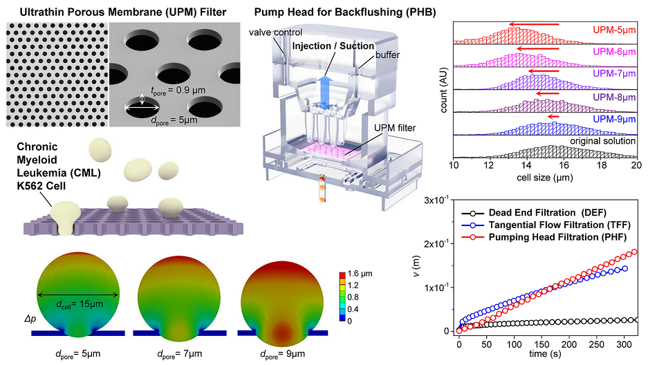
Photographs of the UPM filter are shown in Figure 2a. Si3N4 membranes are arranged in a rectangular array of 10 columns and 13 rows on a 25 × 25 mm silicon substrate. The hexagonal pore arrays are of diameters (dpore) 5, 6, 7, 8, and 9 μm and 0.9 μm in thickness (tpore). The distance between pores was chosen to render the porosity about 32.5%. Each membrane has an area of 0.825 × 0.825 mm, and a pore array was patterned in an active area of 0.7 × 0.7 mm. Therefore, as 130 membranes were used, the total active area was 63.7 mm2. For membranes with 5-μm pores (UPM-5), the total active area was slightly less. Table 2 lists the design values of the UPM filters by the pore sizes and the values measured after fabrication. The measured values were slightly smaller than the design values because the photomask pattern is not accurately transferred to the wafer, given the loading effect that occurs during the fabrication process. [40] Due to the typical negative minus stress applied to the Si3N4 membrane, the probability of membrane breakage in the process was very low at 0.61%, and the broken membrane was sealed through post-treatment. Figure 2b shows a photograph of a UPM filter installed in the filter housing. To eliminate leakage, silicon gaskets were appressed on both sides of the UPM. Figure 2c shows a photograph of the pump head with three input/output ports on the top and 3 × 3 nozzles on the bottom. As shown in the scanning electron micrographs (SEMs) of Figure 2d, the pore side walls are vertical and the diameters rather uniform. The standard deviations of the pore diameters are the error values of Table 2. The membrane aspect ratio, thus the diameter divided by the thickness (dpore/tpore), of UPM-5 is 5.4 but increases to 10.1 for UPM-9. Due to the high aspect ratio, damage applied to cells during filtering can be minimized. Such silicon-based UPM filters are bio-friendly and can be used to prepare transmission electron microscope grids. [41] (More images including cross-sectional view of UPM filter are shown Figure S5.)
The simplest methods that evaluate filter cut-offs use beads. [11,14] In Figure 3a, the size distributions of the four types of beads are shown. The average bead sizes were 5.1, 6.8, 8.9, and 10.6 μm and they were mixed in a single suspension. The software uses the outlines to identify particles that are near-circular, calculates their areas and sizes, and fits the sizes to a Gaussian distribution. Figure 3b-e show the size distributions of beads in the filtrates and retentates when the suspension was filtered through UPM-6, 7, 8, and 9 respectively. Usually, the D90 and D99 values are used to evaluate size separation performance. [42] D99 tends to increase as the pore diameter increases. D99 was 6.2 μm for UPM-6, 7.2 μm for UPM-7, 7.9 μm for UPM-8, and 8.8 μm for UPM-9. Major reductions in the retentate peaks are evident, and the second peak at the 6.8-μm position decreases as the pore diameter increases. The D99s of all UPM filters were repeatedly evaluated, and the averages and standard deviations are presented in Figure 3f. (Further details on determining the size distribution of beads and microscope images of clogged filters are shown in Figures S6–S8.)
Figure 4 shows the filtering results for K562 cells based on the finite element method. Figure 4a-c show the filtrate and retentate particle distributions after filtering. A MATLAB code was written to fit the results to a Gaussian distribution. The filtrate peak downshifted as the pore diameter decreased (Figure 4d). The median values (D50s) of the filtrate distributions corresponding to the various filter pore diameters are shown in Figure 4e. The D50 was 15.7 μm before filtration, and did not change after filtering through UPM-15. However, the values decreased slightly to 15.4 μm after filtering through UPM-9, to 14.7 μm after filtering through UPM-7, and to 13.3 μm after filtering through UPM-5 because the uniform, regular pore arrangements of the UPM filters very effectively fractionate cells [19]; cells can be effectively isolated by controlling pore size. Table 3 and Table 4 list the D10, 50, 90, 95, and 99 values of the original suspension, and those of the filtrates and retentates, by the filter pore diameters. The filtrate distribution is greatly affected by the pore diameter, but the retentate distribution less so. The filter particle recovery rates by the pore diameters are shown in Figure 4f. The particle recovery rate is high in the retentate and low in the filtrate when the pore diameter is small, but high in the filtrate and low in the retentate when the pore diameter is large. However, the total recovery rate is always high, thus 83.6 to 91.3%. (Further result on K562 cells filtration can be found in Figure S9.)
The effect of pore diameter on the pore penetration of K562 cells was investigated via finite element analysis. Figure 4g shows the analytical parameters, thus the cell diameter (dcell), pore diameter (dpore), and the pressure difference (Δp) between the upper and lower sides of the membrane. In fact, positive pressure was applied to the upper sides of the membrane and cell. The effect of applied pressure on the cell penetration length (LP) was calculated for various pore diameters. Figure 4h shows the deformation of cells of diameter 15 μm when passing through membranes with pore diameters of 5, 7, and 9 μm. In all cases, the same pressure difference (140 Pa) was applied. As the pore diameter increases, cell deformation also increases, and therefore also LP. To allow of quantitative analysis, LP was written as a function of Δp (Figure 4i). Note that when the pore diameter is 5 μm, the initial LP is small and then increases slowly with respect to Δp; when the pore diameter is 9 μm, the initial LP is large and increases rapidly with respect to Δp. Thus, as the pore diameter increases, the more readily the cells penetrate the pores, greatly increasing the probability that cells will pass through the filter. The pressure was assumed to be applied to the upper side of the filter, as during experiments. However, a scenario in which suction was applied below the cells was also analyzed; this differed significantly from the pressure-on-top situation, which can be found in Figure S10 of the SI.
Figure 5a shows the principles of TFF and pumping head filtration (PHF). When the three filtering methods were compared, TFF and PHF were significantly better than DEF (Figure 5b). DEF proceeded in a non-pressurized manner; there was no vacuum pump. CML cells are soft, and thus easily damaged by high pressure, undermining the utility of filtering. In the DEF graph, fouling commences within 2 s, thus even under non-pressurized conditions. Based on the measurements and the calculations of Eqs. 2, 4, 6, and 8, both the J0 values and the blocking constants can be obtained using the least squares method (LSM). The validities of the blocking models can be compared by determining the extent of RMSE minimization; the RMSE is:
The DEF result is shown in Figure 5c and is in good agreement with predictions of the intermediate, standard blocking model. Two types of blocking occurred. [43] However, minor differences between the measured J values and those calculated using the fitted parameters are apparent in Figure 5d. The minimized RMSE values are compared in Table 5; these are consistent with the model. Also, the measured data were fitted using the linear regression models of the blocking laws. [26] The inset of Figure 5c shows the linear regression model for standard blocking; the R2 value was 0.988. The inset of Figure 5d shows the linear regression model for intermediate blocking; R2 was 0.989. Figure 5e shows that, during TFF, not only the filtering volume increased but the fouling initiation time was delayed, implying that the filter blocks more slowly even at much higher filtration volumes than that of DEF. Unlike during DEF, flux continues, thus never becoming completely saturated, even after fouling onset [44] (Figure 5a). When the LSM was used to explore the validities of the blocking models, TFF was well-matched to the intermediate blocking model. However, as shown in the inset to Figure 5e, when determining validities using linear regressions, the match to the standard blocking model was also high; R2 was 0.995. The inset of Figure 5f shows the linear regression result for the intermediate blocking model. Qualitatively, the agreement is good, but R2 is low because of data instability.
The DEF and FTT filtering volumes (the v figures) are nonlinear and become saturated with time, but the v for PHF is linear and does not become saturated (Figure 5a and g). When the LSM was used to explore the validities of blocking models, the theoretical curves were in good agreement with the experimental data, but did not indicate a preferred fit for any model. As shown in Figure 5h and the inset, the curve of the filtering rate (the J value) exhibits periodic changes, reflecting episodic backflushing. Thus, the filtering results are difficult to explain using the known blocking mechanisms. Table 5 shows that, even after fitting via linear regression, the R2 values of all four models were less than 0.1, evidencing poor validity. This confirms that PHF cannot be explained by an existing blocking model. Despite this, PHF maintains a constant flow rate by continuously repeating injection and suction, and is far superior to DFF and better than TFF in the long-term.
Figure 6 shows micrographs of fluorescent K562 cells. Figure 6a merges the fluorescent and 4′,6-diamidino-2-phenylindole (DAPI)-stained images of K562 cells. The breakpoint cluster region (BCR) is stained green in Figure 7c. Figure 7d shows the protein-tyrosine protein kinase abl1 gene stained orange. K562 cells are chronic myeloid leukemia (CML) cells. The BCR-ABL gene sequence is created via partial breakage and joining of chromosomes 9 and 22. Thus, BCR-ABL status can be observed using a single filtered cell. [45]
5. Conclusion
We developed a filtration system based on UPMs with pores of diameter 5 to 9 μm and used this to isolate near-circular cells and beads of various sizes. The UPM thickness was 0.9 μm and the pore diameters were very uniform, enabling accurate size cut-off. For filtered beads, the D99 was very close to the pore diameter; for K562 cells, the D99 was significantly greater than the pore diameter because beads are rigid and do not deform whereas cells are soft and easily deformed, allowing them to pass through holes smaller than the cells. Therefore, when isolating cells of a specific diameter, a filter with a pore diameter smaller than the cells is required. As the pore diameter became smaller, the size distributions of cells passing through the filter changed from the original value. Specifically, the D50 value of K562 cells was 15.7 μm but, after filtering through UPM-5, the figure became 13.2 μm. It was thus possible to determine precisely a cut-off yielding a single, soft cell line.
Apart from the precise size cut-off, the system minimizes fouling and is very reproducible. Fouling is reduced via periodic PHB; the UPM is extremely thin, and clogged substances are easily removed. It is difficult to maintain low pressure during DEF and TFF but, in our system, PHB controls pumping to maintain a low pressure, thus minimizing soft cell destruction. The filtering rate is constant long-term. Valid blocking models were developed for DEF, TFF, and PHB filtrations. The CSM software facilitates fast and accurate statistical analysis of the sizes of many cells. The system can be applied to separate not only soft cells but also MVs of various sizes. The economic outlook is good given the accurate separation, high reproducibility, and long-term filter viability.
Supplementary Materials
The following supporting information can be downloaded at: Preprints.org, Figure S1: title; Table S1: title; Video S1: title.
Acknowledgments
This work was supported by a grant from Kyung Hee University in 2020 (KHU-20201096).
References
- Horade, M.; Tsai, C.H.D.; Ito, H.; Kaneko, M. Red Blood Cell Responses during a Long-Standing Load in a Microfluidic Constriction. Micromachines-Basel 2017, 8, 100. [Google Scholar] [CrossRef]
- Shao, H.L.; Chung, J.; Lee, K.; Balaj, L.; Min, C.; Carter, B.S.; Hochberg, F.H.; Breakefield, X.O.; Lee, H.; Weissleder, R. Chip-based analysis of exosomal mRNA mediating drug resistance in glioblastoma. Nat Commun 2015, 6, 6999. [Google Scholar] [CrossRef]
- Rho, J.; Chung, J.; Im, H.; Liong, M.; Shao, H.L.; Castro, C.M.; Weissleder, R.; Lee, H. Magnetic Nanosensor for Detection and Profiling of Erythrocyte-Derived Microvesicles. Acs Nano 2013, 7, 11227–11233. [Google Scholar] [CrossRef]
- Lee, S.; Lee, W.; Kim, H.; Bae, P.K.; Park, J.; Kim, J. Oscillatory flow-assisted efficient target enrichment with small volumes of sample by using a particle-based microarray device. Biosens Bioelectron 2019, 131, 280–286. [Google Scholar] [CrossRef]
- Kim, M.S.; Sim, T.S.; Kim, Y.J.; Kim, S.S.; Jeong, H.; Park, J.M.; Moon, H.S.; Kim, S.I.; Gurel, O.; Lee, S.S.; et al. SSA-MOA: a novel CTC isolation platform using selective size amplification (SSA) and a multi-obstacle architecture (MOA) filter. Lab Chip 2012, 12, 5282–5282. [Google Scholar] [CrossRef]
- Stott, S.L.; Hsu, C.H.; Tsukrov, D.I.; Yu, M.; Miyamoto, D.T.; Waltman, B.A.; Rothenberg, S.M.; Shah, A.M.; Smas, M.E.; Korir, G.K.; et al. Isolation of circulating tumor cells using a microvortex-generating herringbone-chip. P Natl Acad Sci USA 2010, 107, 18392–18397. [Google Scholar] [CrossRef]
- Murlidhar, V.; Zeinali, M.; Grabauskiene, S.; Ghannad-Rezaie, M.; Wicha, M.S.; Simeone, D.M.; Ramnath, N.; Reddy, R.M.; Nagrath, S. A Radial Flow Microfluidic Device for Ultra-High-Throughput Affinity-Based Isolation of Circulating Tumor Cells. Small 2014, 10, 4895–4904. [Google Scholar] [CrossRef]
- Cai, S.; Luo, B.; Jiang, P.P.; Zhou, X.X.; Lan, F.; Yi, Q.Y.; Wu, Y. Immuno-modified superparamagnetic nanoparticles via host-guest interactions for high-purity capture and mild release of exosomes. Nanoscale 2018, 10, 14280–14289. [Google Scholar] [CrossRef]
- Podenphant, M.; Ashley, N.; Koprowska, K.; Mir, K.U.; Zalkovskij, M.; Bilenberg, B.; Bodmer, W.; Kristensen, A.; Marie, R. Separation of cancer cells from white blood cells by pinched flow fractionation. Lab Chip 2015, 15, 4598–4606. [Google Scholar] [CrossRef]
- Shin, S.; Han, D.; Park, M.C.; Mun, J.; Choi, J.; Chun, H.; Kim, S.; Hong, J.W. Separation of extracellular nanovesicles and apoptotic bodies from cancer cell culture broth using tunable microfluidic systems. Sci Rep-Uk 2017, 7, 9907. [Google Scholar] [CrossRef]
- Lee, K.; Shao, H.L.; Weissleder, R.; Lee, H. Acoustic Purification of Extracellular Microvesicles. Acs Nano 2015, 9, 2321–2327. [Google Scholar] [CrossRef]
- Li, P.; Mao, Z.M.; Peng, Z.L.; Zhou, L.L.; Chen, Y.C.; Huang, P.H.; Truica, C.I.; Drabick, J.J.; El-Deiry, W.S.; Dao, M.; et al. Acoustic separation of circulating tumor cells. P Natl Acad Sci USA 2015, 112, 4970–4975. [Google Scholar] [CrossRef]
- Liang, L.G.; Kong, M.Q.; Zhou, S.; Sheng, Y.F.; Wang, P.; Yu, T.; Inci, F.; Kuo, W.P.; Li, L.J.; Demirci, U.; et al. An integrated double-filtration microfluidic device for isolation, enrichment and quantification of urinary extracellular vesicles for detection of bladder cancer. Sci Rep-Uk 2017, 7, 46224. [Google Scholar] [CrossRef]
- Woo, H.K.; Sunkara, V.; Park, J.; Kim, T.H.; Han, J.R.; Kim, C.J.; Choi, H.I.; Kim, Y.K.; Cho, Y.K. Exodisc for Rapid, Size-Selective, and Efficient Isolation and Analysis of Nanoscale Extracellular Vesicles from Biological Samples. Acs Nano 2017, 11, 1360–1370. [Google Scholar] [CrossRef]
- Phuong, N.T.; Andisetiawan, A.; Lam, D.V.; Kim, J.H.; Choi, D.S.; Whang, K.H.; Nham, J.; Lee, Y.J.; Yoo, Y.E.; Yoon, J.S. Nano sand filter with functionalized nanoparticles embedded in anodic aluminum oxide templates. Sci Rep-Uk 2016, 6, 37673. [Google Scholar] [CrossRef]
- Mehendale, N.; Sharma, O.; Pandey, S.; Paul, D. Clogging-free continuous operation with whole blood in a radial pillar device (RAPID). Biomed Microdevices 2018, 20, 75. [Google Scholar] [CrossRef]
- Wunsch, B.H.; Smith, J.T.; Gifford, S.M.; Wang, C.; Brink, M.; Bruce, R.L.; Austin, R.H.; Stolovitzky, G.; Astier, Y. Nanoscale lateral displacement arrays for the separation of exosomes and colloids down to 20 nm. Nat Nanotechnol 2016, 11, 936–940. [Google Scholar] [CrossRef]
- Choi, J.C.; Hyun, J.C.; Yang, S. On-chip Extraction of Intracellular Molecules in White Blood Cells from Whole Blood. Sci Rep-Uk 2015, 5, 15167. [Google Scholar] [CrossRef]
- Sabirova, A.; Pisig, F.; Rayapuram, N.; Hirt, H.; Nunes, S.P. Nanofabrication of Isoporous Membranes for Cell Fractionation. Sci Rep-Uk 2020, 10. [Google Scholar] [CrossRef]
- Mireles, M.; Soule, C.W.; Dehghani, M.; Gaborski, T.R. Use of nanosphere self-assembly to pattern nanoporous membranes for the study of extracellular vesicles. Nanoscale Adv 2020, 2, 4427–4436. [Google Scholar] [CrossRef]
- Mazzocchi, A.R.; Man, A.J.; DesOrmeaux, J.P.S.; Gaborski, T.R. Porous Membranes Promote Endothelial Differentiation of Adipose-Derived Stem Cells and Perivascular Interactions. Cell Mol Bioeng 2014, 7, 369–378. [Google Scholar] [CrossRef]
- Ohanessian, K.; Monnot, M.; Moulin, P.; Ferrasse, J.H.; Barca, C.; Soric, A.; Boutin, O. Dead-end and crossflow ultrafiltration process modelling: Application on chemical mechanical polishing wastewaters (vol 158, pg 164, 2020). Chem Eng Res Des 2020, 162, 38–38. [Google Scholar] [CrossRef]
- Enten, A.C.; Leipner, M.P.I.; Bellavia, M.C.; King, L.E.; Sulchek, T.A. Optimizing Flux Capacity of Dead-end Filtration Membranes by Controlling Flow with Pulse Width Modulated Periodic Backflush. Sci Rep-Uk 2020, 10, 896. [Google Scholar] [CrossRef]
- Karabacak, N.M.; Spuhler, P.S.; Fachin, F.; Lim, E.J.; Pai, V.; Ozkumur, E.; Martel, J.M.; Kojic, N.; Smith, K.; Chen, P.I.; et al. Microfluidic, marker-free isolation of circulating tumor cells from blood samples. Nat Protoc 2014, 9, 694–710. [Google Scholar] [CrossRef]
- Hui, T.H.; Zhou, Z.L.; Qian, J.; Lin, Y.; Ngan, A.H.W.; Gao, H. Volumetric Deformation of Live Cells Induced by Pressure-Activated Cross-Membrane Ion Transport. Phys Rev Lett 2014, 113, 118101. [Google Scholar] [CrossRef]
- Iritani, E.; Katagiri, N. Developments of Blocking Filtration Model in Membrane Filtration. Kona Powder Part J 2016, 179–202. [Google Scholar] [CrossRef]
- Abràmoff, M.D.; Magalhães, P. J.; Ram, S. J. Image Processing with ImageJ. Biophotonics International 2004, 11, 36–42. [Google Scholar]
- Almandoz, C.; Pagliero, C.; Ochoa, A.; Marchese, J. Corn syrup clarification by microfiltration with ceramic membranes. J Membrane Sci 2010, 363, 87–95. [Google Scholar] [CrossRef]
- Li, M.; Liu, L.Q.; Xi, N.; Wang, Y.C.; Dong, Z.L.; Xiao, X.B.; Zhang, W.J. Atomic force microscopy imaging and mechanical properties measurement of red blood cells and aggressive cancer cells. Sci China Life Sci 2012, 55, 968–973. [Google Scholar] [CrossRef]
- Wang, G.H.; Crawford, K.; Turbyfield, C.; Lam, W.; Alexeev, A.; Sulchek, T. Microfluidic cellular enrichment and separation through differences in viscoelastic deformation. Lab Chip 2015, 15, 532–540. [Google Scholar] [CrossRef]
- Li, Y.; Deng, J.X.; Zhou, J.; Li, X.E. Elastic and viscoelastic mechanical properties of brain tissues on the implanting trajectory of sub-thalamic nucleus stimulation. J Mater Sci-Mater M 2016, 27, 163. [Google Scholar] [CrossRef] [PubMed]
- https://www.memsnet.org/material/siliconnitridesi3n4film/.
- Sun, X.H.; Wang, K.; Wu, H.A.; Chen, J.; Long, R. Finite element simulation of a viscoelastic cell entering a cylindrical channel: Effects of frictional contact. Mech Mater 2022, 167, 104263. [Google Scholar] [CrossRef]
- Ruth, B.F. Studies in Filtration III. Derivation of General Filtration Equations. Industrial & Engineering Chemistry 1935, 27, 708–723. [Google Scholar]
- Ruth, B.F. Correlating Filtration Theory with Industrial Practice. Industrial & Engineering Chemistry 1946, 38, 564–571. [Google Scholar]
- Hermans, P.H.; Bredée, H.L. Principles of the mathematical treatment of constant-pressure filtration. Journal of The Society of Chemical Industry 1936, 55, 1–4. [Google Scholar]
- Grace, H.P. Resistance and Compressibility of Filter Cake. Chemical Engineering Progress. Chemical Engineering Progress, 1953, 49, 303–318. [Google Scholar]
- Grace, H.P. Structure and performance of filter media. II. Performance of filter media in liquid service. AIChE Journal 1956, 2, 316–336. [Google Scholar] [CrossRef]
- Hermia, J. Constant pressure blocking filtration laws - Application to power-law non-newtonian fluids. Transaction of the Institution of Chemical Engineers 1982, 60, 183–187. [Google Scholar]
- Mogab, C.J. The loading effect in plasma etching. Journal of The Electrochemical Society 1977, 124, 1262–1268. [Google Scholar] [CrossRef]
- Wolfrum, B.; Mourzina, Y.; Sommerhage, F.; Offenhausser, A. Suspended nanoporous membranes as interfaces for neuronal biohybrid systems. Nano Lett 2006, 6, 453–457. [Google Scholar] [CrossRef]
- Geiss, O.; Bianchi, I.; Senaldi, C.; Bucher, G.; Verleysen, E.; Waegeneers, N.; Brassinne, F.; Mast, J.; Loeschner, K.; Vidmar, J.; et al. Particle size analysis of pristine food-grade titanium dioxide and E 171 in confectionery products: Interlaboratory testing of a single-particle inductively coupled plasma mass spectrometry screening method and confirmation with transmission electron microscopy. Food Control 2021, 120, 107550. [Google Scholar] [CrossRef] [PubMed]
- Amosa, M.K. Towards sustainable membrane filtration of palm oil mill effluent: analysis of fouling phenomena from a hybrid PAC-UF process. Applied Water Science 2017, 7, 3365–3375. [Google Scholar] [CrossRef]
- Hwang, K.J.; Hsu, Y.L.; Tung, K.L. Effect of particle size on the performance of cross-flow microfiltration. Adv Powder Technol 2006, 17, 189–206. [Google Scholar] [CrossRef]
- Druker, B.J.; Tamura, S.; Buchdunger, E.; Ohno, S.; Segal, G.M.; Fanning, S.; Zimmermann, J.; Lydon, N.B. Effects of a selective inhibitor of the Abl tyrosine kinase on the growth of Bcr-Abl positive cells. Nat Med 1996, 2, 561–566. [Google Scholar] [CrossRef] [PubMed]
Figure 1.
Overview of the filtering system and filtering principle: (a) Illustrated diagram for the fabrication process of the UPM filter, (b) the structure of the PHB (upper), mechanism of backflush (right), schematic of the filtering system (lower), (c) illustration of four blocking models: cake filtration, intermediate blocking, standard blocking, and complete blocking.
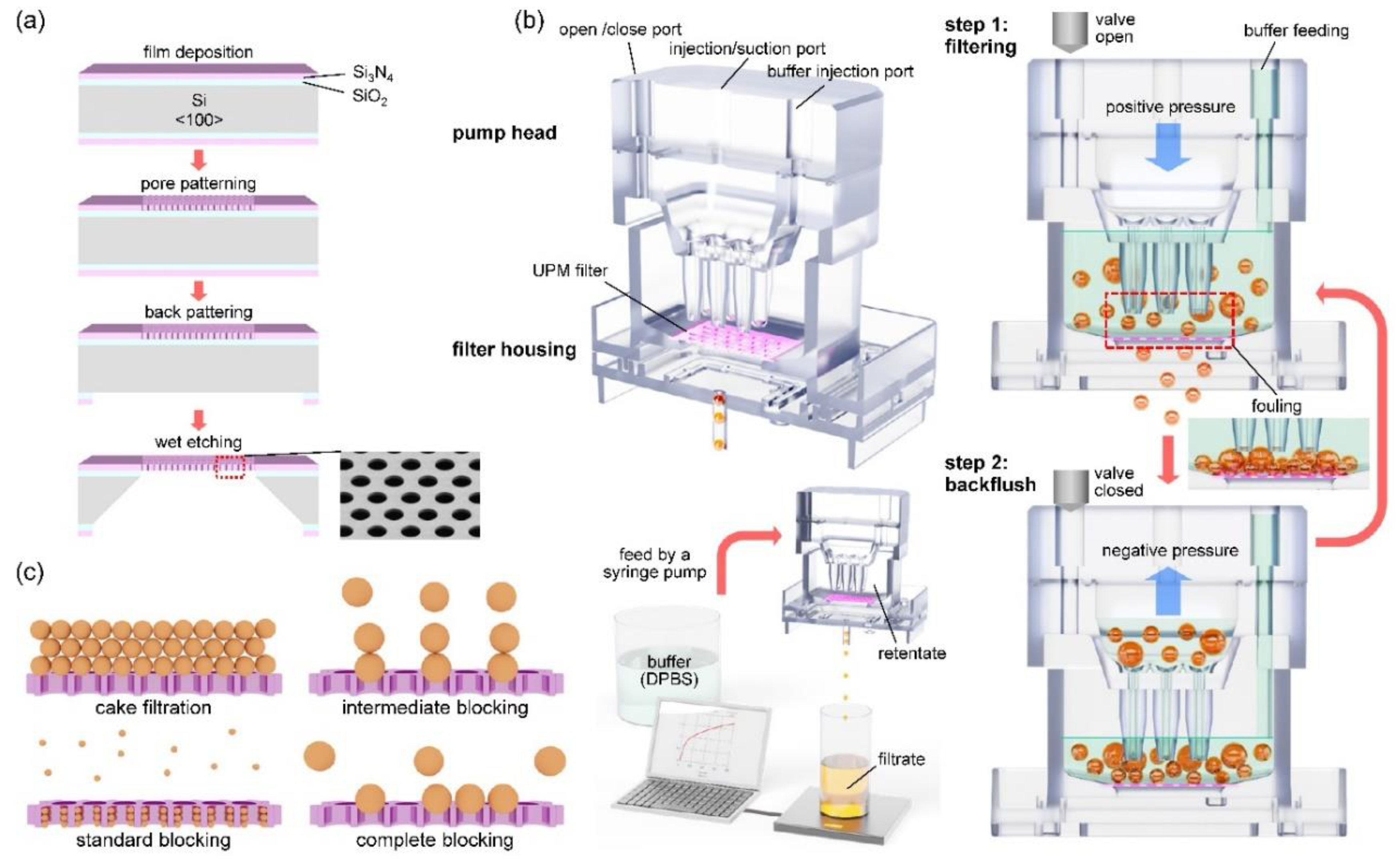
Figure 2.
Structure of UPM filter and PHB: (a) Photo of UPM filter (upper), microscope image showing active area and membrane area (lower), (b) photo of the lower part of PHB (filter housing) with UPM filter installed inside, (c) photo of the upper part of PHB (pump head), (d) SEM images of UPM filter: UPM-5μm (left), UPM-7μm (middle), and UPM-9μm (right) (the scale bar in the upper image represents 50μm and the scale bar in the lower image represent 5μm.).
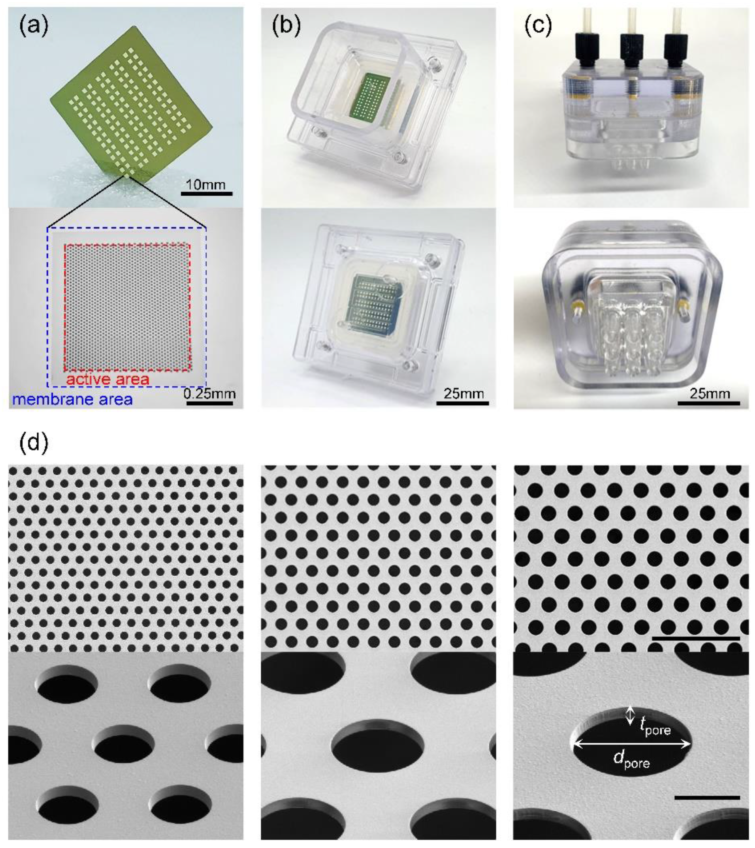
Figure 3.
Filtering result of beads mixture: (a) size distribution of the original beads mixture, (b) size distribution of the filtrate after filtration with UPM-6μm, distribution of retentate (inset), (c) distribution of the filtrate of UPM-7μm, distribution of retentate (inset), (d) distribution of the filtrate of UPM-8μm, distribution of retentate (inset), (e) distribution of the filtrate of UPM-9μm, distribution of retentate (inset), (f) D99 of filtrate as a function of pore diameters.
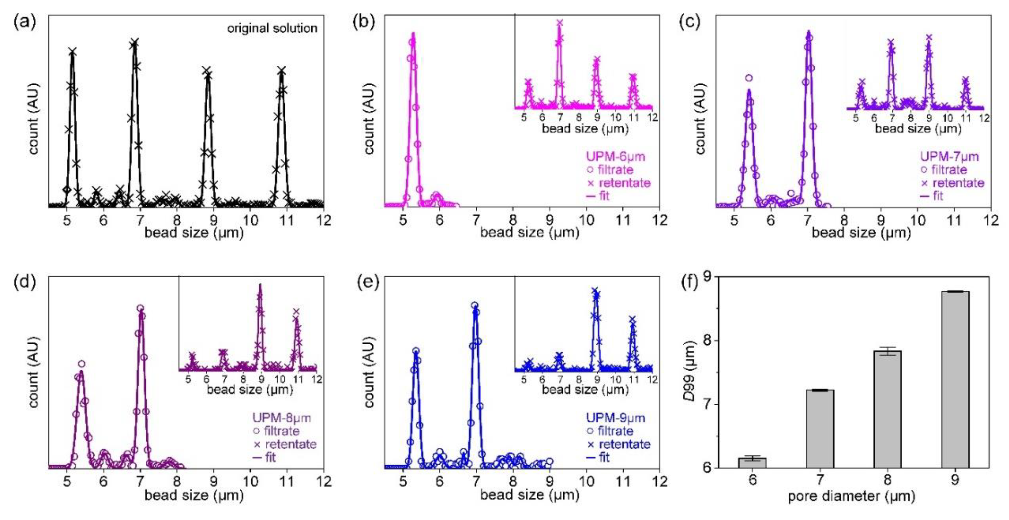
Figure 4.
Filtering result of K562 cell: (a) size distribution of the filtrate and retentate after filtration with UPM-5μm, (b) size distribution of the filtrate and retentate after filtration with UPM-7μm, (c) size distribution of the filtrate and retentate after filtration with UPM-9μm, (d) comparison of size distributions of filtrates from various UPM filters and original solution, (e) D50 of filtrate as a function of pore diameters, (f) recovery rates as a function of pore diameters, (g) modeling parameters of cell entering the pore of the membrane, (h) finite element analysis (FEA) result of deformation of cell entering the pores of different diameters, (i) FEA result of the penetrating length (LP) as a function of the applied pressure (Δp).
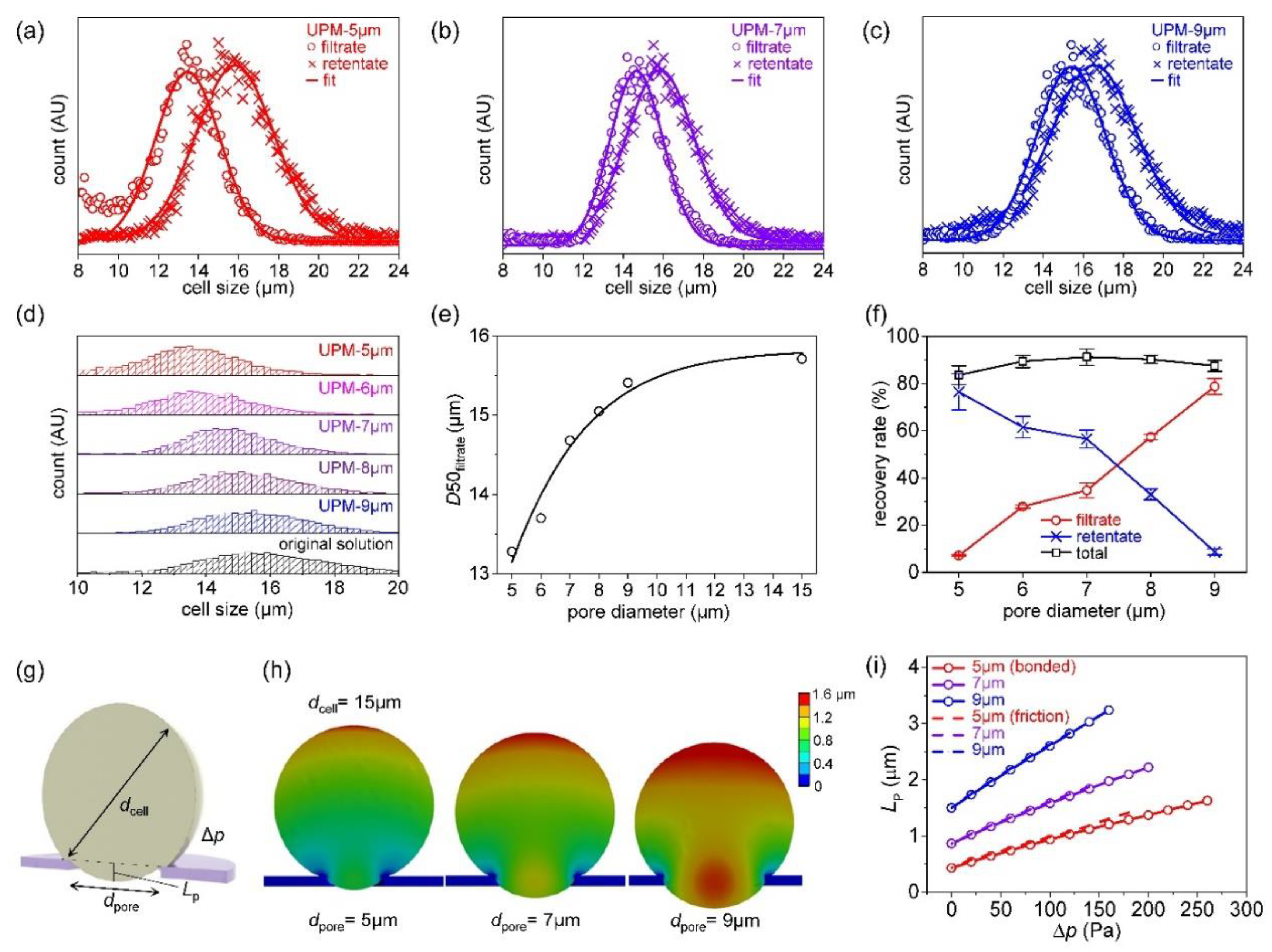
Figure 5.
Analysis of the filtering rate: (a) Illustrated principle of two filtering methods: tangential flow filtration, pumping head filtration, (b) comparison of filtering volume measured from three different filtering methods, (c) filtering volume measured from DEF, calculated curves by four blocking models, the linear regression model for standard blocking (inset), (d) filtering rate measured from DEF, calculated curves by four blocking models, the linear regression model for intermediate blocking (inset), (e) filtering volume measured from TFF, calculated curves by four blocking models, the linear regression model for standard blocking (inset), (f) filtering rate measured from TFF, calculated curves by four blocking models, the linear regression model for intermediate blocking (inset), (g) filtering volume measured from PHF, calculated curves by four blocking models, the linear regression model for cake filtration (inset), (h) filtering rate measured from TFF, calculated curves by four blocking models, two graphs for a specific time (inset).
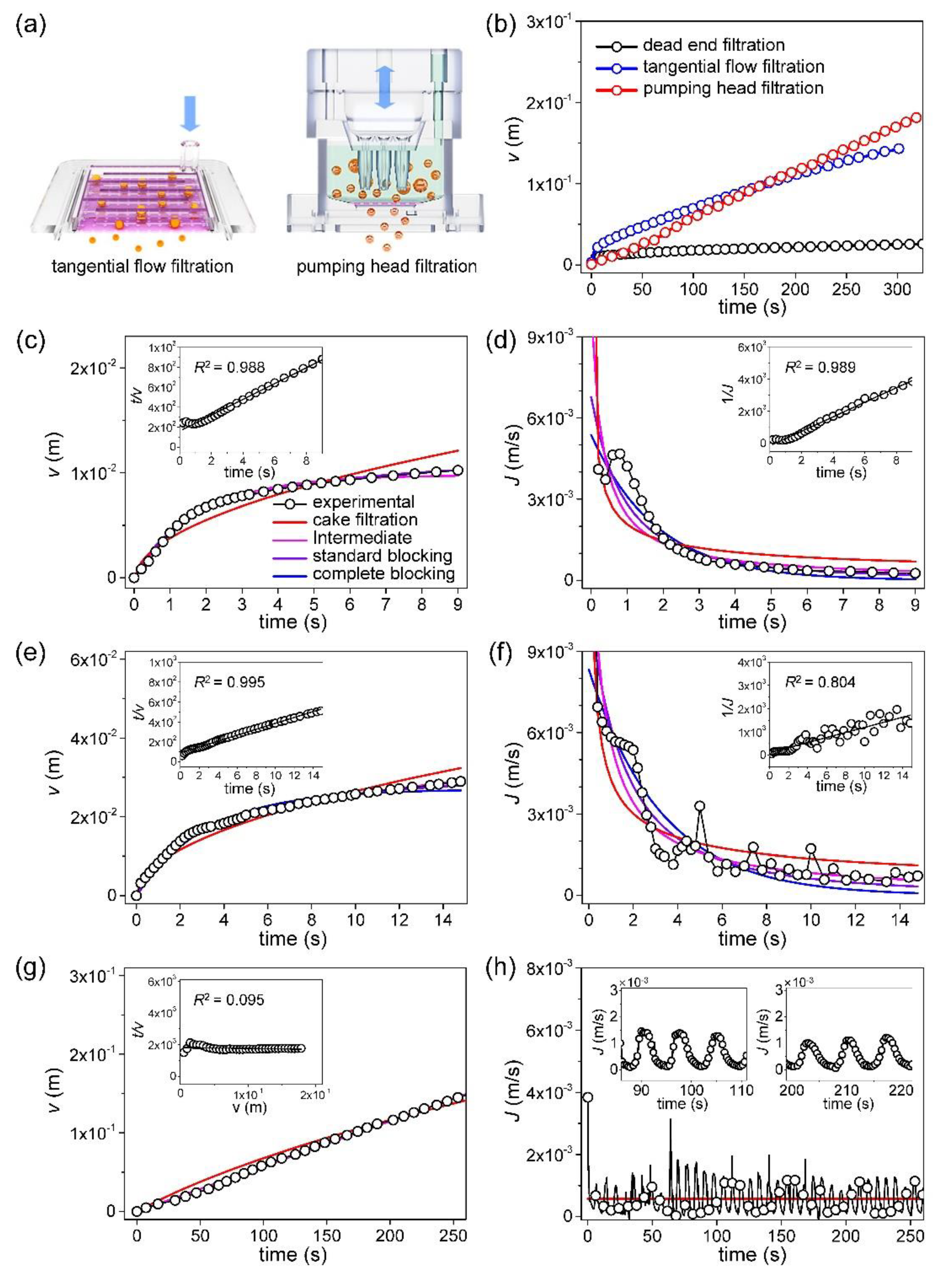
Figure 6.
Florescence microscope image of K562 cell: (a) a merged image of the stained K562 cells, which is stained with 4′,6-diamidino-2-phenylindole (DAPI) by fluorescence microscopy, (b) magnified image of the rectangular part, (c) BCR stained in green color, (d) ABL stained in orange color.
Figure 6.
Florescence microscope image of K562 cell: (a) a merged image of the stained K562 cells, which is stained with 4′,6-diamidino-2-phenylindole (DAPI) by fluorescence microscopy, (b) magnified image of the rectangular part, (c) BCR stained in green color, (d) ABL stained in orange color.
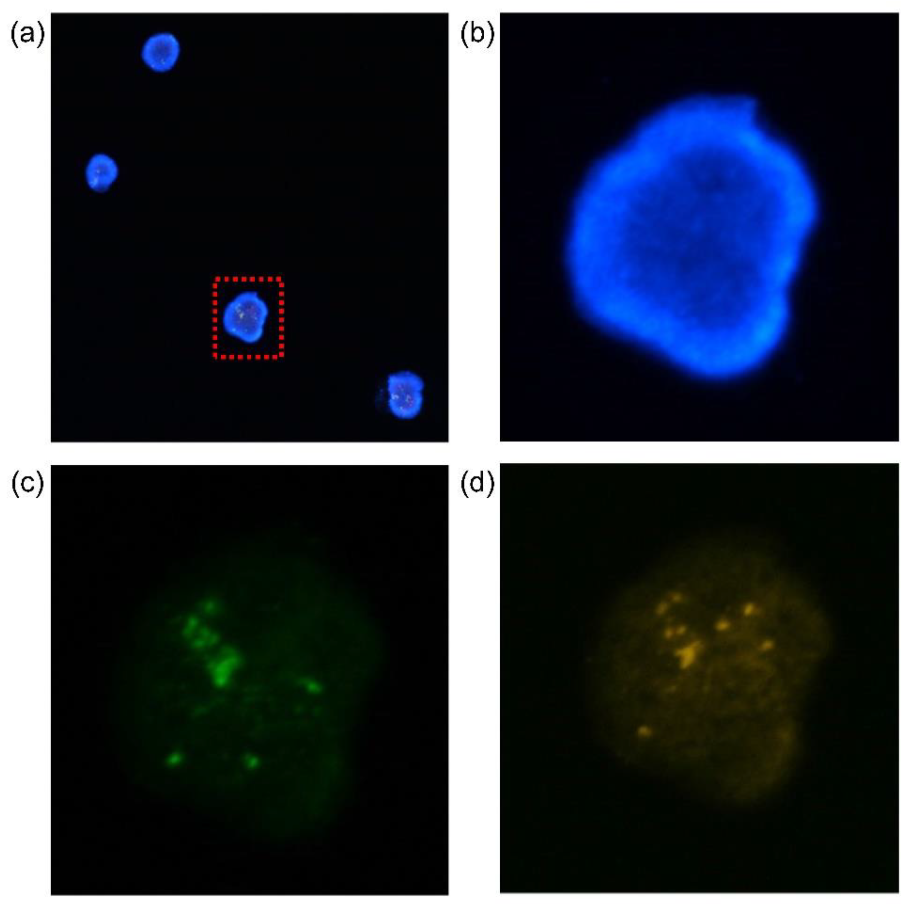

Table 1.
filtrate volume per unit membrane area (ν) and filtration rate (J) for each blocking model.
Table 1.
filtrate volume per unit membrane area (ν) and filtration rate (J) for each blocking model.
| Model | ν(t) | J(t) | blocking constant |
|---|---|---|---|
| Cake filtration | kc | ||
| Intermediate blocking | ki | ||
| Standard blocking | ks | ||
| Complete blocking | kb |
Table 2.
design values of UPM filters according to the pore size and measured values.
| designed pore dia. (μm) | actual pore dia. (μm) | designed porosity (%) | actual porosity (%) | active area (mm2) | thickness (μm) | |
|---|---|---|---|---|---|---|
| UPM-5 | 5 | 4.82 ± 0.13 | 32.6 | 30.3 | 54.9 | 0.89 |
| UPM-6 | 6 | 5.87 ± 0.01 | 32.5 | 31.1 | 63.7 | 0.89 |
| UPM-7 | 7 | 6.83 ± 0.06 | 32.5 | 31.0 | 63.7 | 0.89 |
| UPM-8 | 8 | 7.60 ± 0.04 | 32.6 | 29.6 | 63.7 | 0.89 |
| UPM-9 | 9 | 9.00 ± 0.06 | 32.6 | 32.6 | 63.7 | 0.89 |
Table 3.
D10, 50, 90, 95, and 99 of original solution, and filtrate.
| filtrate | K562 | UPM-5 | UPM-6 | UPM-7 | UPM-8 | UPM-9 | UPM-15 |
|---|---|---|---|---|---|---|---|
| D10 | 13.4 | 10.0 | 11.0 | 13.0 | 12.7 | 13.3 | 13.6 |
| D50 | 15.7 | 13.3 | 13.7 | 14.7 | 15.1 | 15.4 | 15.7 |
| D90 | 18.6 | 15.4 | 15.9 | 16.6 | 17.4 | 17.8 | 18.4 |
| D95 | 19.4 | 16.1 | 16.7 | 17.4 | 18.1 | 18.5 | 19.3 |
| D99 | 22.2 | 17.5 | 18.2 | 18.7 | 19.7 | 20.4 | 22.4 |
Table 4.
D10, 50, 90, 95, and 99 of original solution, and retentate.
| K562 | UPM-5 | UPM-6 | UPM-7 | UPM-8 | UPM-9 | |
|---|---|---|---|---|---|---|
| D10 | 13.4 | 13.5 | 13.7 | 13.8 | 13.4 | 13.6 |
| D50 | 15.7 | 15.8 | 15.9 | 15.8 | 16.0 | 16.6 |
| D90 | 18.6 | 18.9 | 18.8 | 18.5 | 18.9 | 20.0 |
| D95 | 19.4 | 19.7 | 19.8 | 19.5 | 20.0 | 21.6 |
| D99 | 22.2 | 22.4 | 22.8 | 23.2 | 23.6 | 25.5 |
Table 5.
Review of suitability for 4 blocking models for each filtration method.
| Filtration method | Blocking model | fitting result | |||
| Jo (m/s) | blocking constant | fitting method 1: RMSE |
fitting method 2: R2 |
||
| Dead end filtration | cake filtration | 2.46×10⁻² | 3.24×10⁵ (m-2s) | 2.50×10⁻³ | 0.658 |
| intermediate | 1.26×10⁻² | 3.67×10² (m-1) | 3.56×10⁻⁴ | 0.989 | |
| standard | 4.82×10⁻³ | 1.35×10² (m-1) | 7.12×10⁻⁴ | 0.988 | |
| complete | 3.26×10⁻³ | 2.45×10⁻¹ (s-1) | 1.25×10⁻³ | 0.873 | |
| Tangential flow filtration | cake filtration | 9.62×10⁻² | 3.89×10⁴ (m-2s) | 2.68×10⁻³ | 0.893 |
| intermediate | 1.06×10⁻² | 8.91×101 (m-1) | 1.16×10⁻³ | 0.804 | |
| standard | 6.09×10⁻³ | 4.17×101 (m-1) | 2.12×10⁻³ | 0.995 | |
| complete | 4.32×10⁻³ | 1.08×10⁻¹ (s-1) | 3.06×10⁻³ | 0.736 | |
| Pumping head filtration | cake filtration | 5.28×10⁻⁴ | 1.09×10⁻⁶ (m-2s) | 1.24×10⁻³ | 0.095 |
| intermediate | 5.28×10⁻⁴ | 1.07×10⁻¹⁰ (m-1) | 1.24×10⁻³ | 0.011 | |
| standard | 5.74×10⁻⁴ | 2.00×10⁻¹⁴ (m-1) | 1.24×10⁻³ | 0.079 | |
| complete | 5.74×10⁻⁴ | 1.41×10⁻¹² (s-1) | 1.24×10⁻³ | 0.028 | |
Disclaimer/Publisher’s Note: The statements, opinions and data contained in all publications are solely those of the individual author(s) and contributor(s) and not of MDPI and/or the editor(s). MDPI and/or the editor(s) disclaim responsibility for any injury to people or property resulting from any ideas, methods, instructions or products referred to in the content. |
© 2023 by the authors. Licensee MDPI, Basel, Switzerland. This article is an open access article distributed under the terms and conditions of the Creative Commons Attribution (CC BY) license (https://creativecommons.org/licenses/by/4.0/).
Copyright: This open access article is published under a Creative Commons CC BY 4.0 license, which permit the free download, distribution, and reuse, provided that the author and preprint are cited in any reuse.


