Submitted:
04 July 2023
Posted:
05 July 2023
Read the latest preprint version here
Abstract
Solar photovoltaic systems are becoming increasingly popular due to their outstanding environmental, economic, and technical characteristics. To simulate, manage, and control photovoltaic (PV) systems, the primary challenge is identifying unknown parameters accurately and reliably as early as possible using a robust optimization algorithm. This paper proposes a newly developed cheetah optimizer (CO) and improved CO (ICO) to extract parameters from various PV models. This algorithm, inspired by cheetah hunting behavior, includes several basic strategies: searching, sitting, waiting, and attacking. Although this algorithm has shown remarkable capabilities in solving large-scale problems, it needs improvement concerning its convergence speed and computing time. Here, an improved CO (ICO) is presented to identify solar power model parameters for this purpose. Single-, double-, and PV module models are investigated to test ICO's parameter estimation performance. Statistical analysis uses minimum, mean, maximum, and standard deviation. Furthermore, to improve confidence in test results, Wilcoxon and Freidman rank nonparametric tests are also performed. Compared to other state-of-the-art optimization algorithms, the ICO algorithm is proven to be highly reliable and accurate when identifying PV parameters.
Keywords:
Solar energy
; metaheuristics
; optimization
; energy management
; solar cell
; photovoltaic modeling
1. Introduction
A growing number of solar photovoltaic systems are being integrated with electric utilities due to their outstanding environmental, economic, and technical characteristics [1]. The availability of solar radiation in most regions of the world makes solar energy generation and storage systems an attractive option for customers looking for a quick and efficient method of upgrading their electrical systems. In PV systems, solar energy is converted into electricity. In addition to solar radiation and temperature, several other factors affect the capacity of solar energy to generate electricity. As a result, it is essential to analyze how PV systems perform in real time so that they are capable of being optimized, managed, and modeled [2]. Single-diode model (SDM), double-diode model (DDM), and PV module model (PVMM) are typically used despite the existence of many mathematical models for PV nonlinearity. These models must include parameters that can change with environmental changes, faults, and aging [3]. Thus, regardless of the model used, it is essential to accurately determine unknown parameters as early as possible by using a robust optimization algorithm. Therefore, developing an optimization algorithm capable of accurately estimating the properties of PV models using the current-voltage measurements of the PV cell and module is imperative [4].
An optimization problem can be established to extract PV cell and module parameters, which involves the formulation of an objective function and the establishment of a set of constraints. There is noise in the measured current-voltage data. There are, therefore, several local optima in the search space, resulting in a nonlinear and multimodal search space [5], [6]. Deterministic and metaheuristic algorithms are commonly used to solve this challenging optimization problem. The former method makes use of gradient information, as well as initial points. As a result, classical techniques are ineffective in identifying the parameters of photovoltaic models due to their non-linear and non-convex nature [7]–[9]. There is a consensus that metaheuristic algorithms are more modern and easier to use than deterministic algorithms. Since then, there has been an increase in interest in metaheuristic algorithms for optimizing PV systems more efficiently and flexibly.
The field of study has been subjected to extensive research in recent years. Various metaheuristic and analytical methods have been employed by researchers in order to estimate the parameters of the solar cell/module. They are performance-guided JAYA (PGJAYA) algorithm [6], differential evolution (DE) [10], genetic algorithms (GA) [11], particle swarm optimization (PSO) [12], war strategy optimization (WSO) algorithm [13], SEDE [14], an efficient salp swarm-inspired algorithm (SSA) [15], improved JAYA (IJAYA) [16], RAO [17], modified artificial bee colony (MABC) [18], improved mosth-flame optimization (IMFO) [19], Shuffled frog leaping algorithm (SFLA) [20], triple-phase teaching-learning-based optimization (TPTLBO) [21], improved chaotic whale optimization (ICWO) algorithm [22], Sine-cosine algorithm (SCA) [23], a new hybrid algorithm based on grey wolf optimizer and cuckoo search (GWO-CS) [24], Coyote optimization algorithm (COA) [25], Marine predators algorithm (MPA) [26], adaptive genetic algorithm (AGA) based multi-objective optimization [27], an improved equilibrium optimizer (IEO) [28], new stochastic slime mould algorithm (SMA) [29], and orthogonally adapted Harris hawks optimization (OAHHO) [30], An overview of some of these research papers is presented in Table 1.
Although researchers are developing and modifying meta-heuristic algorithms in light of the “No Free Lunch” theorem [31] to determine the parameters of PV models. According to the authors’ knowledge, past algorithms have not provided a satisfactory balance between accuracy and reliability while maintaining a reasonable computing time. To improve the performance of metaheuristic algorithms, new ideas must be developed to produce simple and efficient methods for dealing with practical optimization problems.
Recently, Akbari et. al., [32] introduced a new and powerful algorithm namely the CO algorithm, which is inspired by the behavior of cheetahs during the hunting process. However, it is necessary to test the performance of this algorithm on different optimization problems so that its strengths are known more, and its weaknesses are also identified and resolved. In this article, this algorithm is utilized for the first time to identify PV parameters. Based on the experiences of the authors, this algorithm has a relatively high computational volume, and its complexity needs to be simplified to be used in optimization problems.
The purpose of this article is to introduce a simplified and improved version of CO, namely ICO, that can improve the features of CO while requiring significantly less computational effort. As part of the ICO algorithm, the search phase is controlled according to the position of the leader, and its step length is also adjusted following the sorted population. This new operator also aids the algorithm’s global search in addition to the local search. In addition, the interaction factor in the attack phase is adjusted based on the prey position, and the turning factor is controlled by a random value. It is believed that the proposed attack operator will improve the behavior of the algorithm in the global search as well as its convergence speed. When it comes to estimating optimal parameters for PV cells and models, the CO and proposed ICO are compared to two recently well-established algorithms for parameter extraction of PV models, i.e., PGJAYA [6] and SEDE [14], and eight well-known original algorithms, i.e., DE [33], PSO [34], GA [35], TLBO [36], JAYA [37], SSA [38], WSO [13], GWO [39].
Following is a summary of an overview of the remainder of the paper. In section 2, we describe in detail the SDM, DDM, and PVMM. The proposed ICO algorithm is presented in section 3. A simulation and evaluation of the results of the experiment are presented in Section 4. Finally, section 5 makes some closing remarks.
2. PV Modeling and Problem Formulation
In the literature, many PV models are presented to describe the characteristics of solar cells and PV module models. Among these models are SDM, DDM, and PVMM. This section describes the mathematical model used to formulate the optimization problem of determining the optimal parameters for these models.
2.1. The Model of a Solar Cell
2.1.1. SDM
For demonstrating the real-time characteristics of PV systems, their mathematical modeling is required by practical considerations. A PV array can be modeled using the cell as its basic unit. SDMs are widely used due to their simplicity and ease of implementation. According to Figure 1(a), the equivalent circuit for the SDM consists of a parallel resistor, a series resistor, a diode, and a current source. Calculating the output current can be accomplished using the following formula [22]:
Where, , , and are, respectively, the photogenerated, shunt resistor, and diode currents.
Calculating and can be accomplished using Kirchhoff’s Voltage Law (KVL) and Shockley’s equation as follows:
here, represents the non-physical diode ideality factor, whereas represents the diode reverse saturation current; represents cell output voltage; represent shunt resistance; and represents the series resistance.
The junction thermal voltage can be calculated using the electron charge, ( C), the junction temperature, , and Boltzmann’s constant, (J/K), as follows:
Combining Equations (3) to (6) will result in the cell output current () for SDM as follows:
2.1.2. DDM
Although it is widely employed to simulate PV cells, SDM ignores recombination current in the depletion region. As shown in Figure 1(b), by combining the photo-generated current source, the shunt resistance, two rectifying diodes, and the series resistance, DDM can solve the problem.
Using KCL, one can calculate the output current in DDM as follows:
Current flows through the first and second diodes (i.e., and ) as described by the Shockley diode equations in (9) and (10). Diodes also have two ideality factors known as and . Diffusion and saturation currents are and . Thus, substituting (5), (9) and (10), (8) can be rewritten as follows:
2.2. PVMM
A photovoltaic module may be designed to increase voltage and current by arranging several PV cells in parallel or series (see Figure 1(c)). Using the PVMM, the output current can be calculated as follows:
Here, a parallel arrangement consists of M solar cells, and a series arrangement consists of N solar cells.
2.3. Problem Formulation
The goal of the proposed optimization problem is to determine unknown parameters of PV cells and module accurately. An optimization algorithm is commonly employed to minimize the differences between the estimated and experimental I-V data obtained from the PV systems. Hence, as a rule, it is common to consider that the minimization of root mean square error (RMSE) is an objective function that should be considered when determining an estimate of current.
Subject to:
S is the number of experimental paired sample data. and are the s-th measured sample, and the determined value of PV output current, respectively. Constraints (14) indicate the upper () and lower () bounds on the PV parameters (decision variables). For the SDM and PVMM five unknown parameters are , and seven decision variables, i.e., should be defined for the DDM using an optimization technique. Finally, the calculated PV output current in each sample s, , can be expressed using (15), (16), and (17) for SDM, DDM, and PVMM, respectively.
3. Proposed Optimization Algorithm
3.1. Overview of CO Algorithm
Akbari et al. [23] recently developed the CO algorithm as a powerful optimization algorithm for mimicking specific cheetahs’ hunting strategies. This algorithm utilizes three important strategies: searching for prey, sitting and waiting, and attacking. The algorithm introduces leaving the prey and returning home to avoid getting stuck in local optimal points. In this section, the mathematical model of the CO algorithm is explained, then the ICO algorithm is presented.
Based on these strategies, as shown in Figure 2, cheetah populations are formed in different arrangements. The probable hunting arrangements of each cheetah are considered equivalent to the solution to the problem. It is assumed that the best position among the population determines the prey (best solution). Cheetahs adjust their possible arrangements to optimize their performance during the hunting period.
3.1.1. Searching Strategy
A cheetah scans its surroundings or searches for suitable prey based on environmental conditions and hunting behavior. A mathematical model’s searching phase looks like this [23]:
So that represents the current arrangement and represents the new arrangement of cheetah at hunting time . The inverse of a normally distributed random number represents the randomization parameter. Besides, the random step length is defined by , where is expressed for the leader as follows [23]:
where and are the upper and lower limits of the variable . The length of a hunting time is represented by . For other members of a group of cheetahs, the random step length is expressed based on the distance of the cheetah and arbitrarily selected cheetah in a group as follows [23]:
3.1.2. Sitting-and-Waiting Strategy
Cheetahs are swift hunters. During the chase, speed and flexibility require much energy. Therefore, the duration of the attack and chase cannot be long. As a result, one of the important strategies of cheetahs during the hunting process is to wait until the prey is close enough to them. Then, they start the attack. Hunting success can be increased by this behavior, which is modeled as follows [23]:
3.1.3. Attacking Strategy
At the appropriate time, cheetahs attack their prey. Speed and flexibility are two critical factors that the cheetah exploits during its attack. Cheetahs attack with maximum speed so that the cheetah must reach a close distance from their prey in the shortest possible time. In this case, the prey notices the cheetah’s attack and starts to run away. Because of the cheetah’s high speed and short distance from the prey, the prey prefers to escape by changing directions suddenly. Therefore, the cheetah uses its high flexibility to place the prey in unstable conditions and catch it. Attacks may take place individually or in groups. In solo attack mode, the cheetah’s position change is adjusted based on the position of the prey. This can be done interactively in a group attack based on the status of other members of the group and the prey. This strategy can be expressed using the following mathematical model [23]:
where is the prey position; is the turning factor which reflects the sudden changes of the prey while fleeing; and is a randomly chosen value from a normal distribution. The interaction factor is defined by in (22) which is expressed as follows [23]:
3.1.4. Strategy Selection Mechanism
Choosing the right strategy in the CO algorithm is done randomly [23]. Let and be two random numbers from a uniform distribution. If is greater than , the sit-and-wait strategy is selected; otherwise, one of the search or attack strategies takes place. There is a condition between the two strategies of search and attack, which is controlled based on the H factor (see Figure 3). This factor decreases with time, which is expressed as follows [23]:
where is a random value from [0, 1]. A condition has been set between these two strategies so that searching is the most likely choice at the start of hunting season. An attack will likely occur as the time of hunting progresses.
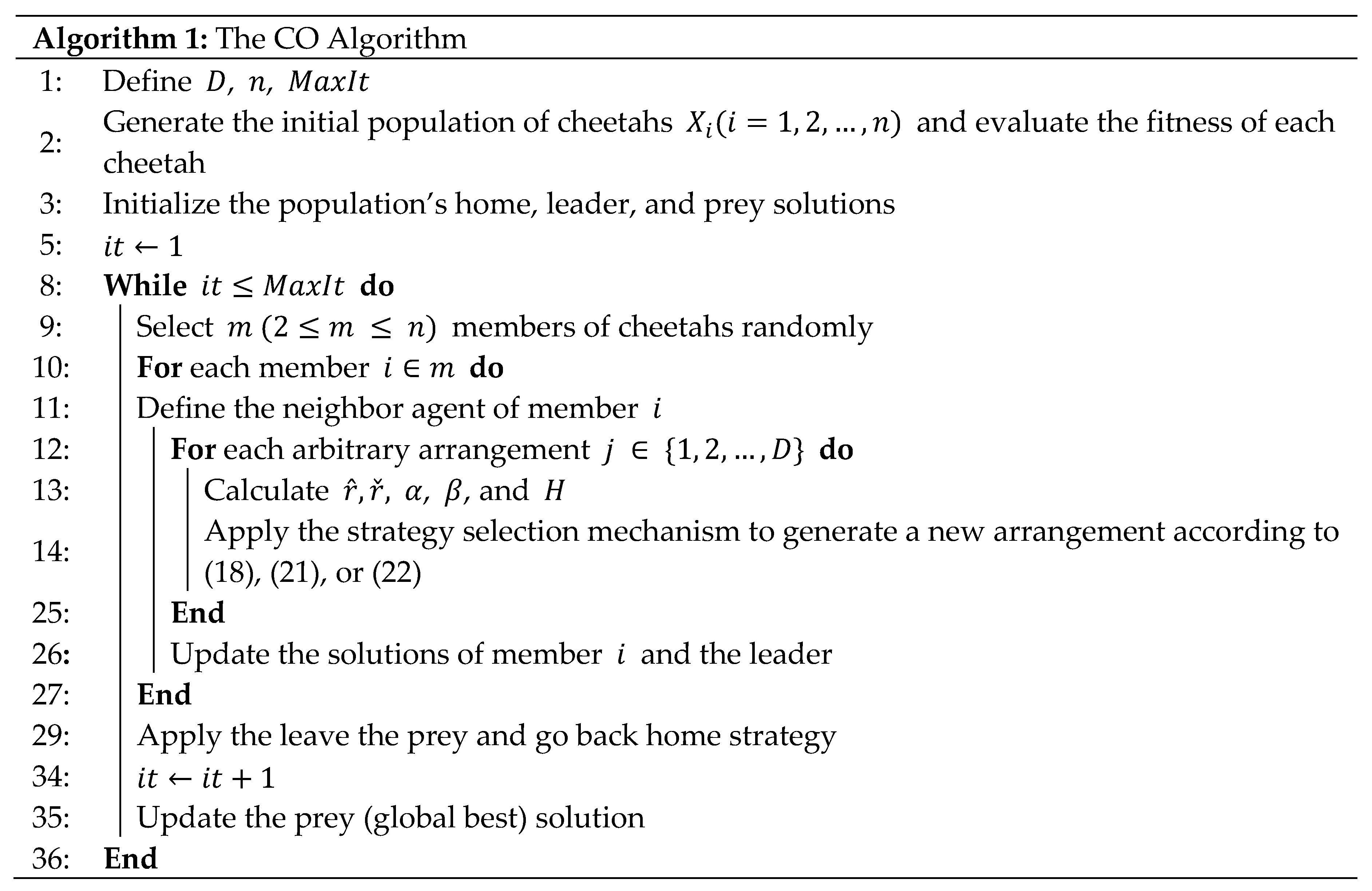
The pseudo-code of CO is summarized in Algorithm 1 [23].
3.2. Improved Cheetah Optimizer (ICO) Algorithm
The CO algorithm has shown good capabilities in solving large-scale problems. However, as will show in the experimental results, it needs improvement in terms of convergence speed and computing time in identifying the parameters of photovoltaic models. For this purpose, a modified version of the CO algorithm is presented to cover these shortcomings.
3.2.1. Searching Strategy
In the search mode of the CO algorithm, each cheetah updates its position based on its previous position. This is when cheetahs usually follow the leader of the group and follow him. On this basis, the searching strategy in (18) is modified based on the leader position (second-best cheetah’s position in the population), , as follows:
where, the randomization parameter (), and random step length () are modified as follows:
Here, and are random values of the normal distribution function. and are the position of k’th and i’th cheetahs in the sorted population.
It is worth noting that updating the position of each cheetah around the position of the group leader can help the local search phase. In addition, the second term on the right side of the relationship (26) causes the diversity of solutions and thus contributes to the global search phase (exploitation phase). Also, by creating long steps during the hunting period, the random parameter will cause the solution to go out of the range of variables and thus be replaced with the new random solution in the population. Consequently, in addition to diversifying the solutions, it can prevent the algorithm from getting stuck in local optimal points.
3.2.2. Attacking Strategy
Moreover, the attacking strategy in the ICO algorithm is reformulated as follows:
where is a random value from [0, 1].
In the CO algorithm, the interaction factor is expressed using the position of the adjacent cheetah (see Eq. (24)). While cheetahs usually attack their prey singly. Therefore, their position should be adjusted based on the position of the prey. Hence, in this proposed attack strategy, each cheetah updates his/her position relative to the prey during the attack mode and moves towards it, which is defined as follows:
This proposed attack strategy helps the CO algorithm to find the near-optimal solution faster. Therefore, the local search capability (exploitation phase) of the CO algorithm is enhanced and its convergence speed will be increased.
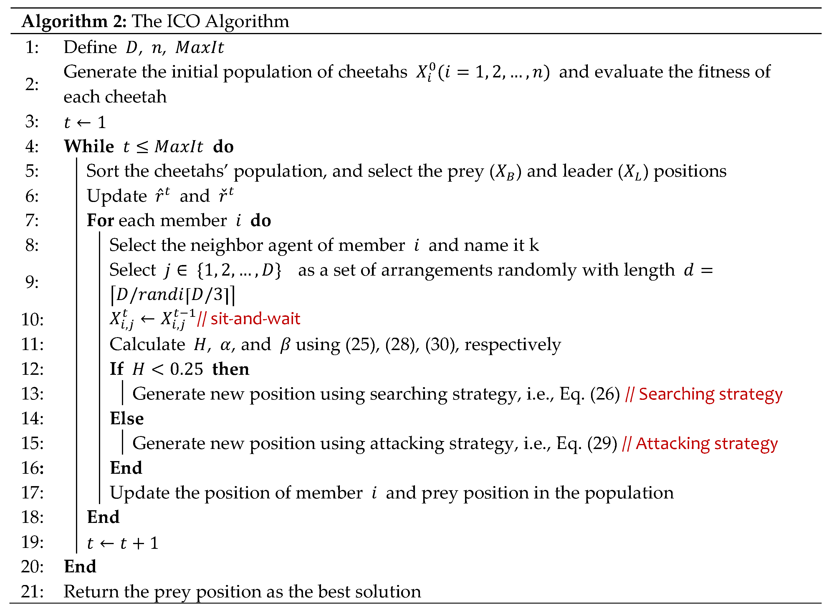
The pseudo-code of the proposed ICO is summarized in Algorithm 2.
4. Experimental Results
The CO and ICO algorithms are evaluated in this section to show their performance on the parameter estimation of three types of PV models, i.e., SD, DD, and PVM models. The SD and DD tests are conducted on silicon solar cells with 57 mm diameters (R.T.C. France) to collect current-voltage data [24]. Moreover, under 1000 W/m2 irradiance, a PV module (Photo Watt-PWP 201) with 36 polycrystalline PV cells is used [24]. Experimental data is used to estimate the parameters of PV models using a variety of algorithms. The maximum and minimum limit for each parameter of the PV model is given in Table 2 [7].
Moreover, two recently developed algorithms including PGJAYA [1] and SEDE [4], as well as eight well-known original algorithms, i.e., DE [25], PSO [26], GA [27], TLBO [28], JAYA [29], SSA [30], WSO [5], GWO [31] are chosen to validate and verify the effectiveness of CO and ICO for identifying PV parameters. The maximum number of 50000 function evaluations is assumed for all case studies. As in the original literature, the other parameters of the applied algorithms are maintained. The statistical analysis is performed by running each algorithm 30 times independently in MATLAB 2021b.
4.1. Population Size Analysis
One of the parameters influencing the performance of any evolutionary algorithm is the size of the initial population. Therefore, the behavior of the proposed algorithm for optimal extraction of the parameters of three PV models has been investigated with the population size (n) of 10, 20, 40, 50, 80, and 100. For each of these population sizes, the ICO has been run 30 times and the statistical results are summarized in Table 3. As can be seen, for the SD and PVM models, the algorithm can achieve the best solution (Min value) for all population sizes. For the DD model, the algorithm has reached the best solution in 9.824849E-04 with n = 80. In addition, the proposed algorithm shows significant robustness with all initial populations except population 10. The CPU times and Friedman test results through 30 runs are represented in the last three columns of this Table 3, and their average values for the three models are shown in Figure 4. Based on these results, it can be seen that the proposed algorithm with n = 80 has the best relative performance in three models with average sum rank of 80 and CPU time of 39.5 sec. The population size of 40 and 50 rank second and third among all examined population sizes, respectively.
In addition, the convergence characteristics of the algorithm with different population numbers are shown in Figure 5 for three models. When the population number is set above 10, almost the same convergence behavior is seen. However, for the first model, when the population is 40, the speed of convergence is almost better. When the population of 80 and 100 is considered, the speed of convergence in the second model is the best. For the third model, all populations except 100 have almost converged on the same point. For the population number of 10, the speed of convergence in SDM and DDM shows the worst situation among the tested populations, while for the third model, it shows a significant convergence behavior.
4.2. Results of Parameter Extraction Based on SDM
For the SDM, the best solutions found by competitive algorithms with n = 40 and n = 80 including PV parameters and objective function (RMSE) values are summarized in Table 4. From the results, for the two tested population sizes, the best RMSE value of 9.860218778914E–04 is obtained from CO and ICO. For n = 40, SEDE and WSO, and for n = 80, WSO gives the second-best solutions. It should be noted that the lower values of the RMSE indicate a higher accuracy of the estimation of model parameters. The curves of current and power in terms of voltage are illustrated in Figure 6(a) and Figure 6(b) to verify the accuracy of the algorithm. Additionally, the values of IAEI and IAEP are drawn in Figure 6(c) and Figure 6(d) over the voltage ranges. In all cases, the individual absolute error of current (IAEI) is less than 2.52E–3 and the individual absolute error of power (AIEP) is less than 1.375E–3, indicating that CO and ICO are highly accurate in estimating SDM parameters.
4.3. Results of Parameter Extraction Based on DDM
The best solutions found by competitive algorithms for DDM models with n = 40 and n = 80, including PV parameters and optimal RMSE values, are represented in Table 5. From the table, it can be seen that CO obtains the best RMSE value of 9.824848822723E–04 for n = 40, followed by the ICO with RMSE of 9.824860991382E–04. Additionally, for n = 80, these optimizers get the best results out of 12 algorithms. Conversely, SSA and GWO produce the worst results. Figure 7(a) and Figure 7 (b) respectively illustrate the I–V and P–V curves using measured and estimated data for the DDM model. The corresponding IAEI and IAEP are illustrated in Figure 7(c) and Figure 7(d) indicating that CO and ICO are incredibly accurate in estimating DDM parameters.
4.4. PVMM-Based Photo Watt-PWP 201
For PVMM, it can be observed from Table 6 that the best solutions are obtained from CO, ICO, SEDE, and WSO. However, in terms of RMSE, the best result is related to CO, and then ICO, WSO, and SEDE are placed in the next ranks respectively. Among competitive algorithms, for n = 40 and n = 80, CO, ICO, and WSO show stable behavior in finding the best optimal solution. From Figure 8(a) and (b), I–V and P–V characteristics of measured data are very similar to those obtained by ICO and CO. It can be seen that the IAEI and IAEP in this example are less than 0.0048 and 0.0798, respectively (see Figure 8(c) and (d)). The results of this study demonstrate the high accuracy of the estimated parameters by the CO and ICO for the PVMM.
4.5. Comparison of Statistical Results
For a clearer understanding of the comparison, the statistical results are also saved. We record the maximum (Max), the minimum (Min), the mean (Mean), and the standard deviation (SD) of RMSE over thirty independent runs for each algorithm. By comparing the Min, Mean, and SD values of RMSE, one can measure the accuracy, the average accuracy, and the robustness of the applied algorithms. Table 7, Table 8 and Table 9 present the statistical results for 12 algorithms with n = 40 and n = 80 through 30 runs to identify unknown parameters of three PV models. A bolded value indicates the algorithm that produced the best results. A Freidman test is used to determine the performance ranking of the comparative algorithms. In Freidman, the smallest value of mean/sum rank indicates that the applied algorithm is superior to the other 12 algorithms. To measure the significance between ICO and its competitors, the Wilcoxon signed rank test [54] is used with a significance level of 0.05. The symbols of “+” and “≈” in Table 7, Table 8 and Table 9 indicate ICO’s performance is significantly superior and almost similar to its competitor.
For SDM, as shown in Table 7, when n = 40, the ICO, CO, and SEDE give the best and average accuracy results in terms of Min and Mean values. However, in terms of robustness, ICO with an SD value of 3.091E–17 shows the best performance among competitive algorithms. PGJAYA and WSO show the second- and third-best accuracy, respectively. According to the Friedman test, CO shows the best performance and ICO the second-best performance among 12 algorithms, respectively. Besides, when n = 80, ICO and CO show the best accuracy and WSO shows the second-best accuracy. However, in terms of reliability, ICO and CO respectively with the SD values of 5.21E–17 and 1.02E–16 are the best and second best among competitive algorithms. Based on the Wilcoxon signed rank test, there is no significant difference between ICO and CO, while they obtain significantly superior results than other competitive algorithms.
When it comes to DDM, as represented in Table 8, CO results in the best accuracy and ICO obtains the best average accuracy among the tested algorithms. ICO’s accuracy in terms of the minimum value of RMSE is very similar to the result of CO, and other algorithms are unable to approach it. ICO and CO rank first and second in terms of robustness. In addition, when the population size is set at 40, SEDE provides the best performance and ICO provides the second-best performance based on Friedman’s test. When n = 80, however, ICO is determined to be the best-performing algorithm, while CO is determined to be the second-best-performing algorithm among the 12 competing algorithms. Furthermore, when the population size is 40, the Wilcoxon signed rank test does not indicate a significant difference between ICO, CO, SEDE, and PGJAYA. Moreover, based on Wilcoxon tests of n = 80, ICO, CO, and PGJAYA perform similarly.
The best results are from utilizing ICO, CO, and SEDE for PVMM when looking at Min and Mean RMSE of Table 9. Despite WSO’s ability to achieve the highest accuracy, its average accuracy and robustness cannot compete with, ICO, CO, and SEDE. The lowest SD value is achieved by SEDE equals 2.319E–17, and the second and third-best values are obtained by ICO and CO, which achieved 4.998E–17 and 1.105E–16, respectively. According to Friedman’s test, ICO provides the best performance and CO provides the second-best performance when n = 40. For n = 80, this ranking is shifted. The final ranking of comparative algorithms for identifying the unknown parameters of SDM, DDM, and PVMM is shown in Figure 9. For these models, the best sum-ranking result among 12 algorithms with n = 40 is obtained by ICO, followed by CO and SEDE. While n = 80, respectively CO, ICO, and PGJAYA exhibit first, second, and third sum-ranking results in three models.
Additionally, Figure 10 shows a box plot diagram of all competitive algorithms for a visual representation of the distribution of optimal RMSE obtained for three investigated models during 30 runs. Based on the distribution of answers, it is clear that the ICO and CO perform the best in terms of robustness in finding the optimal solution. SEDE and PGJAYA also provide acceptable robustness.
4.6. Computational Time
To further evaluate the performance of competing algorithms, we recorded the computing time for 30 runs of each algorithm on three models and presented them in Figure 11. As can be seen from this figure, different times were spent to identify the parameters of each model of the algorithm. Among the 12 algorithms, GA takes the longest time to solve three models, while JAYA takes the least time for SDM and DDM. Besides, SSA requires the least computational time to solve PVMM, followed by GWO, JAYA, and ICO. For SDM, after JAYA, ICO requires the least computing time. DDM, PSO, GWO, WSO, and SSA have almost the same computing time, and ICO needs a little more time than them. As compared to the original algorithms such as JAYA, GWO, WSO, and SSA, the time spent by ICO is comparable. Its superior performance over these algorithms, however, is significant from a statistical perspective. In addition, although CO, SEDE, and PGJAYA show significant performance in terms of statistical results, they require more computational time than ICO. As compared to CO, the main advantage of ICO is its ability to reduce computing time while maintaining or even improving its performance.
4.7. Convergence Characteristics
According to Figure 12, each algorithm’s convergence curve is depicted for each model and indicates the average RMSE performance across 30 independent runs. As can be seen from Figure 12, it is evident that ICO achieves a competitive or faster convergence rate than other algorithms for three PV models, demonstrating its capability to maintain a good balance between exploration and exploitation. It is worth noting that, the convergence behavior of CO seems better than other conventional algorithms such as DE, GA, PSO, WGO, SSA, TLBO, JAYA, and WSO.
4.8. Exploration and Exploitation Analysis
Keeping exploration and exploitation in balance can be achieved by ensuring sufficient diversity among individuals. In this way, an algorithm can avoid being trapped in a local solution and ultimately produce a better solution to a particular optimization problem. However, exploration-exploitation and diversity measurements alone can’t prove that one algorithm is better than another for solving optimization problems. Some experiments are presented in this section to evaluate exploration-exploitation and diversity of solutions in the comparative algorithms on the SDM problem. During iterations, Figure 13 shows variations in exploration, exploitation, and population diversity among individuals of competitive algorithms. Calculations are made under the procedure detailed in [32].
Figure 13(a) and (b) shows that, in contrast to other algorithms, SSA and GWO exhibit a greater percentage of exploration during iterations than exploitation. It is shown in Figure 14 that these two algorithms have average exploration-exploitation ratios of 80%:20% and 76%:24%. This is due to the high diversity in the population in these two algorithms as shown in Figure 13(c). Comparatively, GA and WSO provide the greatest level of exploitation capabilities, with an average value of 99%. Further evidence of this can be found in Figure 13(c), demonstrating that these two algorithms were unable to provide sufficient diversity throughout the iteration process. Thus, premature convergence is one of the main weaknesses of these algorithms.
Figure 13(a) and (b) also show that ICO, CO, DE, PSO, GA, TLBO, SEDE, JAYA, PGJAYA, and WSO are all explorative at first, but after a few iterations, they are deemed exploitative algorithms. Similar results can be observed for the diversity measure in these algorithms which after a few iterations, it drops (see Figure 13(c)). It must be noted, however, that spikes in the population diversity characteristic are observed in CO due to the leave the prey and go back home strategy.
5. Conclusion
This paper introduced a simplified and improved version of the CO algorithm and investigated its performance in identifying unknown parameters of PV cells and modules. An extensive set of experiments was conducted to assess the performance of CO and ICO in identifying parameters of different PV models, including SDM, DDM, and PVMM. It examined how the size of the initial population affects the performance of ICO. It was found that the algorithm performed well for populations with a number greater than 10. The results obtained from ICO and CO were also compared to those obtained from other well-known algorithms in terms of accuracy, robustness, computing time, and convergence characteristics. Based on the Wilcoxon signed rank test and Friedman test, the performance of the algorithms was compared and determined. The results of these tests indicated the superiority of ICO compared to other competitive algorithms. Moreover, the further improvement made in CO revealed that ICO was able to significantly reduce computing time by maintaining or improving its features, and it also demonstrated enhanced performance. ICO will be applied in future studies to solve a variety of power system optimization problems, including placement of renewable distributed generations, economic load dispatch, and feeder reconfiguration.
Author Contributions
All the authors contributed to formulating the research idea, algorithm design, result analysis, writing and reviewing the research. All authors have read and agreed to the published version of the manuscript.
Data Availability Statement
Data sharing is not applicable—no new data was generated.
Acknowledgments
This work has been funded by Ajman University under the internal research grant (2022-IRG-ENIT-9).
Conflicts of Interest
The authors declare no conflict of interest.
References
- Yu, K.; Qu, B.; Yue, C.; Ge, S.; Chen, X.; Liang, J. A Performance-Guided JAYA Algorithm for Parameters Identification of Photovoltaic Cell and Module. Appl. Energy 2019, 237, 241–257. [Google Scholar] [CrossRef]
- Ishaque, K.; Salam, Z. An Improved Modeling Method to Determine the Model Parameters of Photovoltaic (PV) Modules Using Differential Evolution (DE). Sol. energy 2011, 85, 2349–2359. [Google Scholar] [CrossRef]
- Khanna, V.; Das, B.K.; Bisht, D.; Singh, P.K. A Three Diode Model for Industrial Solar Cells and Estimation of Solar Cell Parameters Using PSO Algorithm. Renew. Energy 2015, 78, 105–113. [Google Scholar] [CrossRef]
- Liang, J.; Qiao, K.; Yu, K.; Ge, S.; Qu, B.; Xu, R.; Li, K. Parameters Estimation of Solar Photovoltaic Models via a Self-Adaptive Ensemble-Based Differential Evolution. Sol. Energy 2020, 207, 336–346. [Google Scholar] [CrossRef]
- Ayyarao, T.S.L. V; Kumar, P.P. Parameter Estimation of Solar PV Models with a New Proposed War Strategy Optimization Algorithm. Int. J. Energy Res. 2022, 46, 7215–7238. [Google Scholar] [CrossRef]
- Abbassi, R.; Abbassi, A.; Heidari, A.A.; Mirjalili, S. An Efficient Salp Swarm-Inspired Algorithm for Parameters Identification of Photovoltaic Cell Models. Energy Convers. Manag. 2019, 179, 362–372. [Google Scholar] [CrossRef]
- Yu, K.; Liang, J.J.; Qu, B.Y.; Chen, X.; Wang, H. Parameters Identification of Photovoltaic Models Using an Improved JAYA Optimization Algorithm. Energy Convers. Manag. 2017, 150, 742–753. [Google Scholar] [CrossRef]
- Premkumar, M.; Babu, T.S.; Umashankar, S.; Sowmya, R. A New Metaphor-Less Algorithms for the Photovoltaic Cell Parameter Estimation. Optik (Stuttg). 2020, 208, 164559. [Google Scholar] [CrossRef]
- Jamadi, M.; Merrikh-Bayat, F.; Bigdeli, M. Very Accurate Parameter Estimation of Single-and Double-Diode Solar Cell Models Using a Modified Artificial Bee Colony Algorithm. Int. J. Energy Environ. Eng. 2016, 7, 13–25. [Google Scholar] [CrossRef]
- Sheng, H.; Li, C.; Wang, H.; Yan, Z.; Xiong, Y.; Cao, Z.; Kuang, Q. Parameters Extraction of Photovoltaic Models Using an Improved Moth-Flame Optimization. Energies 2019, 12, 3527. [Google Scholar] [CrossRef]
- Hasanien, H.M. Shuffled Frog Leaping Algorithm for Photovoltaic Model Identification. IEEE Trans. Sustain. Energy 2015, 6, 509–515. [Google Scholar] [CrossRef]
- Liao, Z.; Chen, Z.; Li, S. Parameters Extraction of Photovoltaic Models Using Triple-Phase Teaching-Learning-Based Optimization. IEEE Access 2020, 8, 69937–69952. [Google Scholar] [CrossRef]
- Oliva, D.; Abd El Aziz, M.; Hassanien, A.E. Parameter Estimation of Photovoltaic Cells Using an Improved Chaotic Whale Optimization Algorithm. Appl. Energy 2017, 200, 141–154. [Google Scholar] [CrossRef]
- Montoya, O.D.; Gil-González, W.; Grisales-Noreña, L.F. Sine-Cosine Algorithm for Parameters’ Estimation in Solar Cells Using Datasheet Information. In Proceedings of the Journal of Physics: Conference Series; 2020; Vol. 1671, p. 12008. [Google Scholar]
- Long, W.; Cai, S.; Jiao, J.; Xu, M.; Wu, T. A New Hybrid Algorithm Based on Grey Wolf Optimizer and Cuckoo Search for Parameter Extraction of Solar Photovoltaic Models. Energy Convers. Manag. 2020, 203, 112243. [Google Scholar] [CrossRef]
- Diab, A.A.Z.; Sultan, H.M.; Do, T.D.; Kamel, O.M.; Mossa, M.A. Coyote Optimization Algorithm for Parameters Estimation of Various Models of Solar Cells and PV Modules. Ieee Access 2020, 8, 111102–111140. [Google Scholar] [CrossRef]
- Soliman, M.A.; Hasanien, H.M.; Alkuhayli, A. Marine Predators Algorithm for Parameters Identification of Triple-Diode Photovoltaic Models. IEEE Access 2020, 8, 155832–155842. [Google Scholar] [CrossRef]
- Kumari, P.A.; Geethanjali, P. Adaptive Genetic Algorithm Based Multi-Objective Optimization for Photovoltaic Cell Design Parameter Extraction. Energy Procedia 2017, 117, 432–441. [Google Scholar] [CrossRef]
- Abdel-Basset, M.; Mohamed, R.; Mirjalili, S.; Chakrabortty, R.K.; Ryan, M.J. Solar Photovoltaic Parameter Estimation Using an Improved Equilibrium Optimizer. Sol. Energy 2020, 209, 694–708. [Google Scholar] [CrossRef]
- Kumar, C.; Raj, T.D.; Premkumar, M.; Raj, T.D. A New Stochastic Slime Mould Optimization Algorithm for the Estimation of Solar Photovoltaic Cell Parameters. Optik (Stuttg). 2020, 223, 165277. [Google Scholar] [CrossRef]
- Jiao, S.; Chong, G.; Huang, C.; Hu, H.; Wang, M.; Heidari, A.A.; Chen, H.; Zhao, X. Orthogonally Adapted Harris Hawks Optimization for Parameter Estimation of Photovoltaic Models. Energy 2020, 203, 117804. [Google Scholar] [CrossRef]
- AlRashidi, M.R.; AlHajri, M.F.; El-Naggar, K.M.; Al-Othman, A.K. A New Estimation Approach for Determining the I–V Characteristics of Solar Cells. Sol. Energy 2011, 85, 1543–1550. [Google Scholar] [CrossRef]
- Akbari, M.A.; Zare, M.; Azizipanah-Abarghooee, R.; Mirjalili, S.; Deriche, M. The Cheetah Optimizer: A Nature-Inspired Metaheuristic Algorithm for Large-Scale Optimization Problems. Sci. Rep. 2022, 12, 1–20. [Google Scholar] [CrossRef]
- Easwarakhanthan, T.; Bottin, J.; Bouhouch, I.; Boutrit, C. Nonlinear Minimization Algorithm for Determining the Solar Cell Parameters with Microcomputers. Int. J. Sol. energy 1986, 4, 1–12. [Google Scholar] [CrossRef]
- Storn, R.; Price, K. Differential Evolution--a Simple and Efficient Heuristic for Global Optimization over Continuous Spaces. J. Glob. Optim. 1997, 11, 341–359. [Google Scholar] [CrossRef]
- Kennedy, J.; Eberhart, R. Particle Swarm Optimization. In Proceedings of the Proceedings of ICNN’95-international conference on neural networks; pp. 199541942–1948.
- Mitchell, M. An Introduction to Genetic Algorithms; MIT press, 1998. [Google Scholar]
- Rao, R.V.; Savsani, V.J.; Vakharia, D.P. Teaching–Learning-Based Optimization: An Optimization Method for Continuous Non-Linear Large Scale Problems. Inf. Sci. (Ny). 2012, 183, 1–15. [Google Scholar] [CrossRef]
- R. Venkata Rao Jaya: A Simple and New Optimization Algorithm for Solving Constrained and Unconstrained Optimization Problems. Int. J. Ind. Eng. Comput. 2016, 7, 19–34. [Google Scholar] [CrossRef]
- Mirjalili, S.; Gandomi, A.H.; Mirjalili, S.Z.; Saremi, S.; Faris, H.; Mirjalili, S.M. Salp Swarm Algorithm: A Bio-Inspired Optimizer for Engineering Design Problems. Adv. Eng. Softw. 2017, 114, 163–191. [Google Scholar] [CrossRef]
- Mirjalili, S.; Mirjalili, S.M.; Lewis, A. Grey Wolf Optimizer. Adv. Eng. Softw. 2014, 69, 46–61. [Google Scholar] [CrossRef]
- Hussain, K.; Salleh, M.N.M.; Cheng, S.; Shi, Y. On the Exploration and Exploitation in Popular Swarm-Based Metaheuristic Algorithms. Neural Comput. Appl. 2019, 31, 7665–7683. [Google Scholar] [CrossRef]
Figure 1.
Equivalent representation of the (a) SDM, (b) DDM, and (c) PVMM.
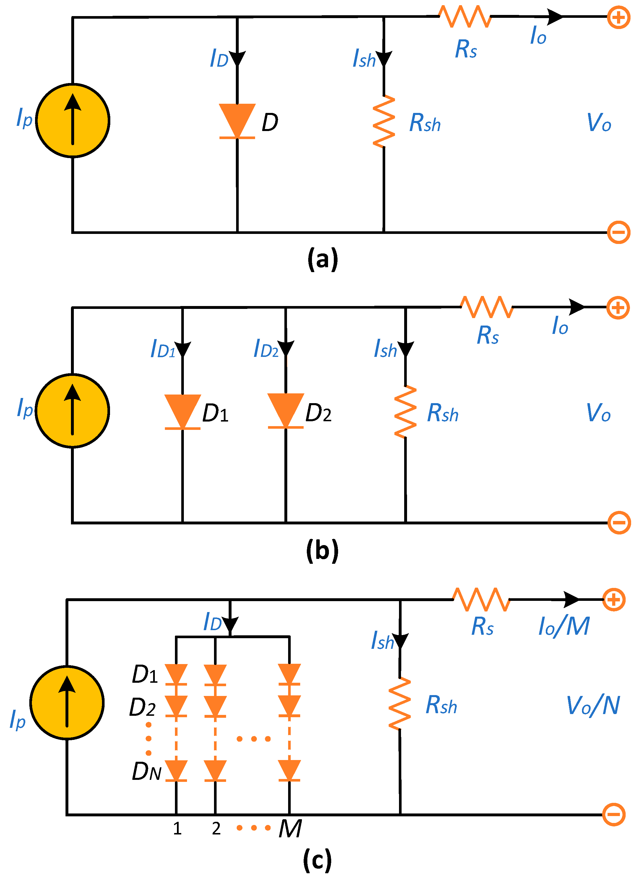
Figure 2.
Representation of the CO algorithm.
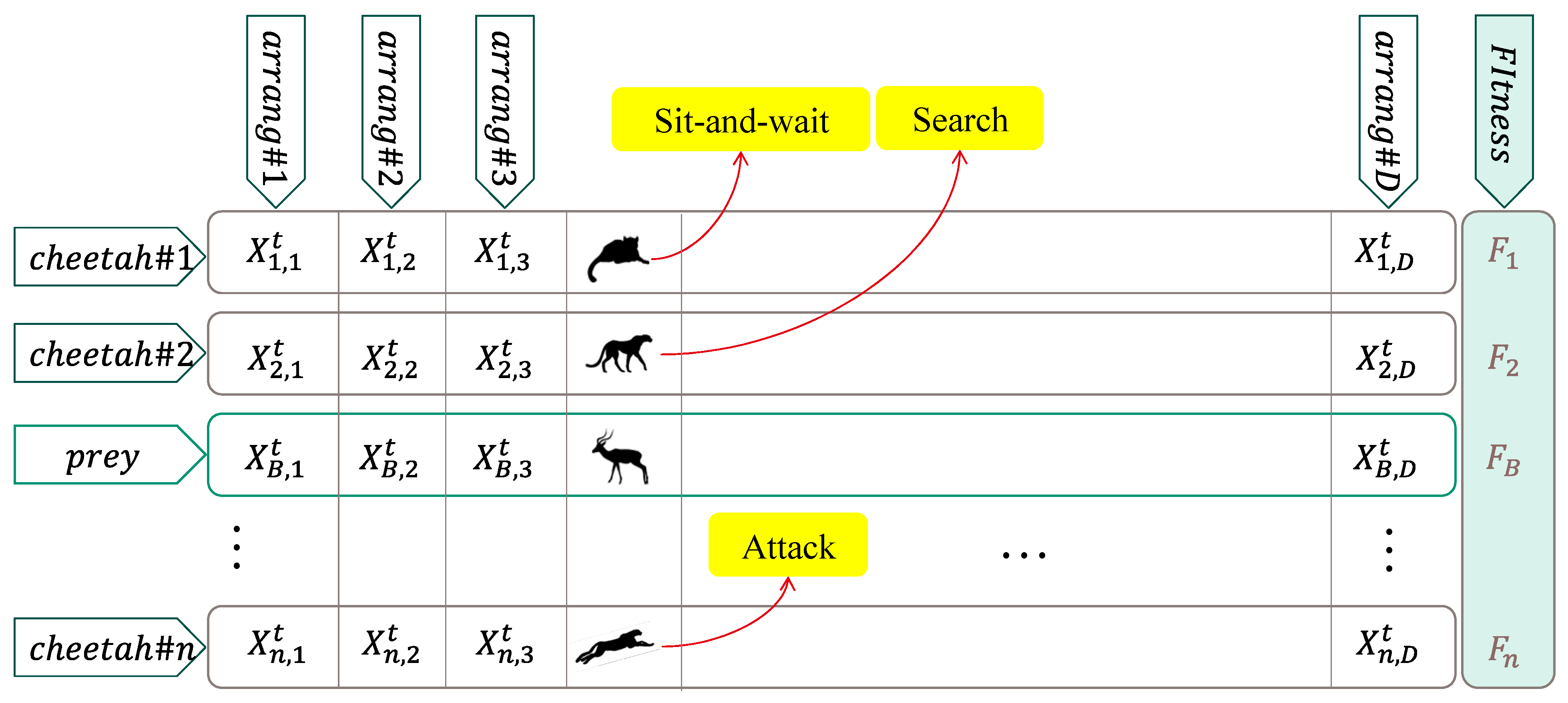
Figure 3.
An overview of the strategy selection mechanism in the CO algorithm.
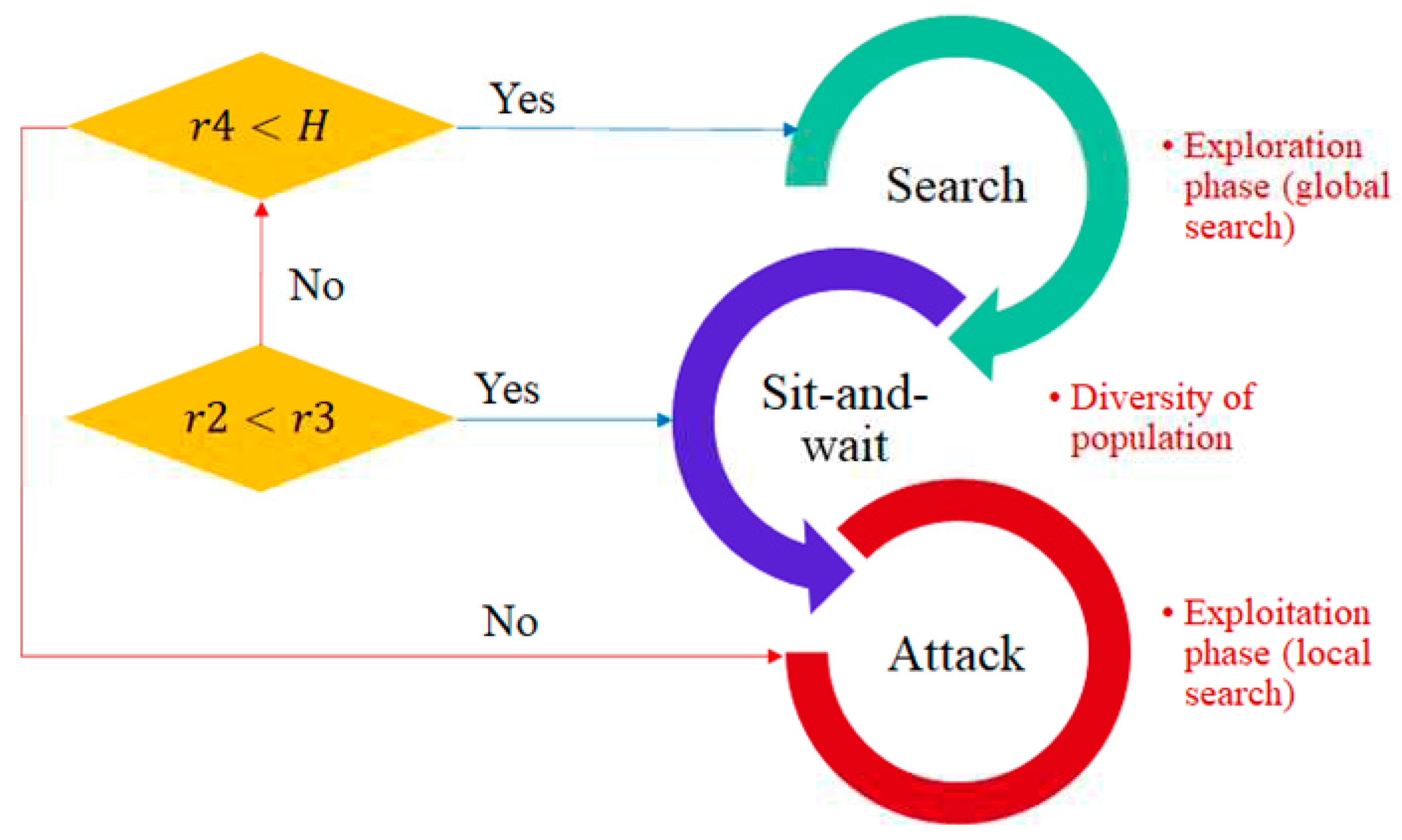
Figure 4.
Average ranks of the utilized population sizes in three models.
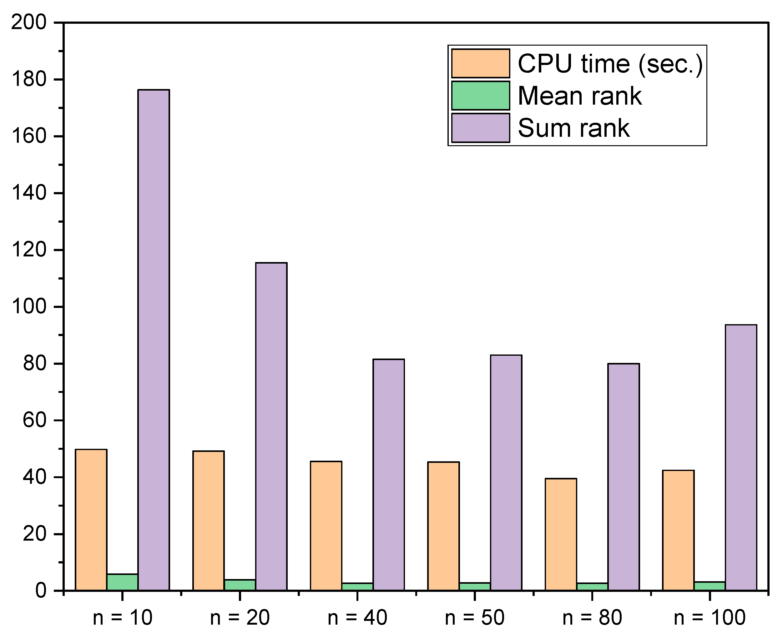
Figure 5.
Convergence curves of ICO with different population sizes in solving (a) SDM, (b) DDM, and (c) PVMM.
Figure 5.
Convergence curves of ICO with different population sizes in solving (a) SDM, (b) DDM, and (c) PVMM.
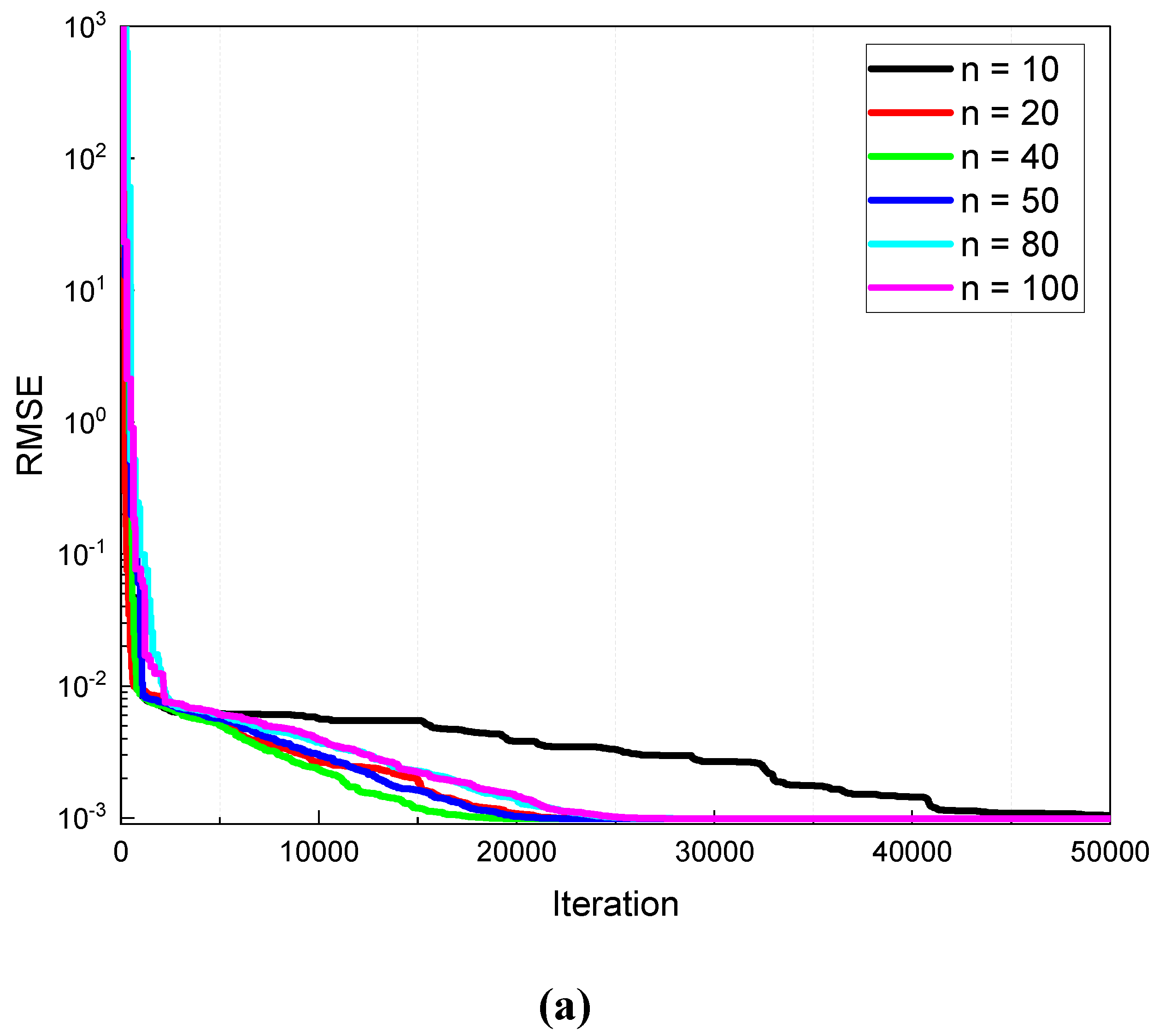
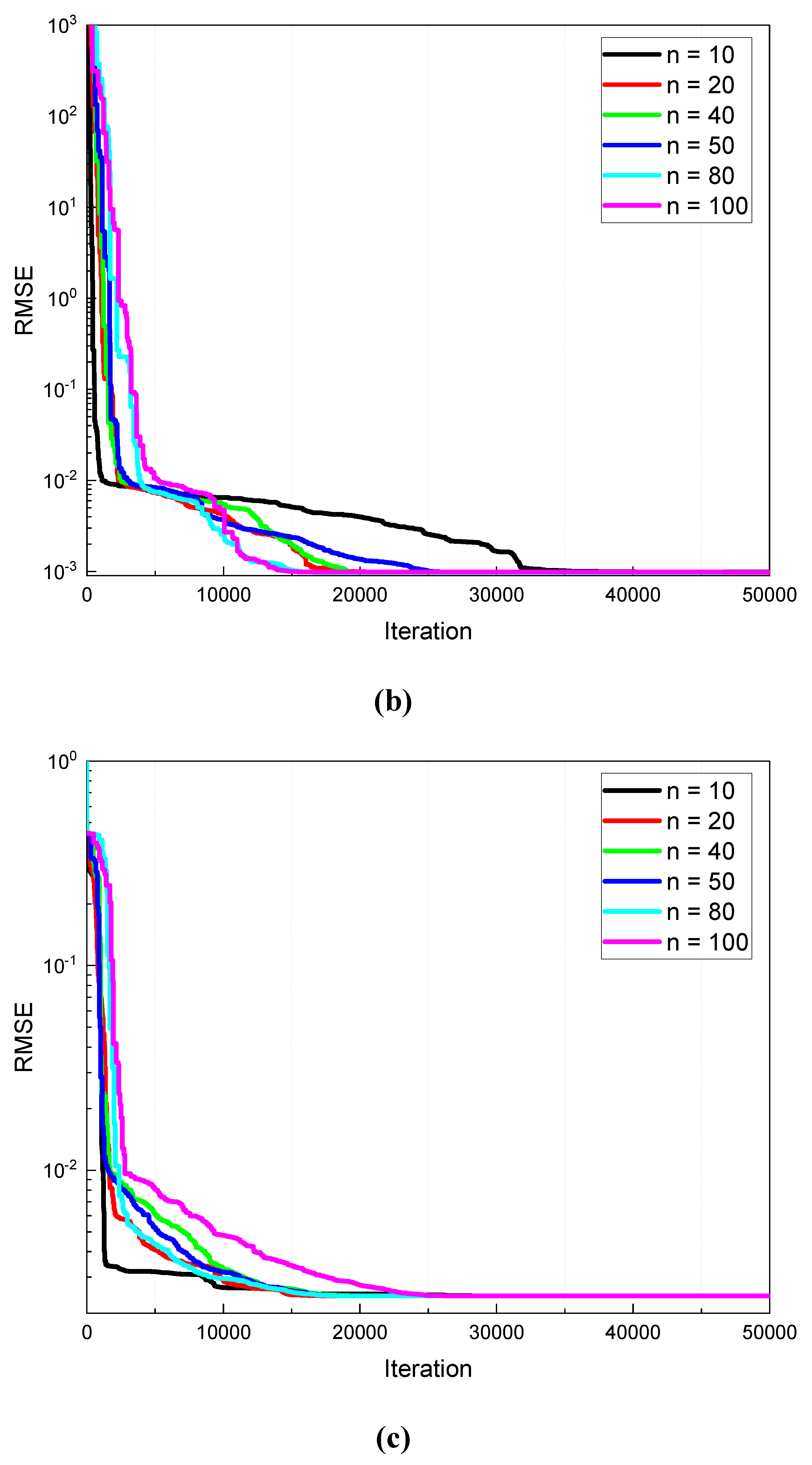
Figure 6.
Estimated and measured data of the RTC France silicon solar cell based on the SDM by ICO; (a) I–V, (b) P–V, (c) IAEI, and (d) IAEP.
Figure 6.
Estimated and measured data of the RTC France silicon solar cell based on the SDM by ICO; (a) I–V, (b) P–V, (c) IAEI, and (d) IAEP.
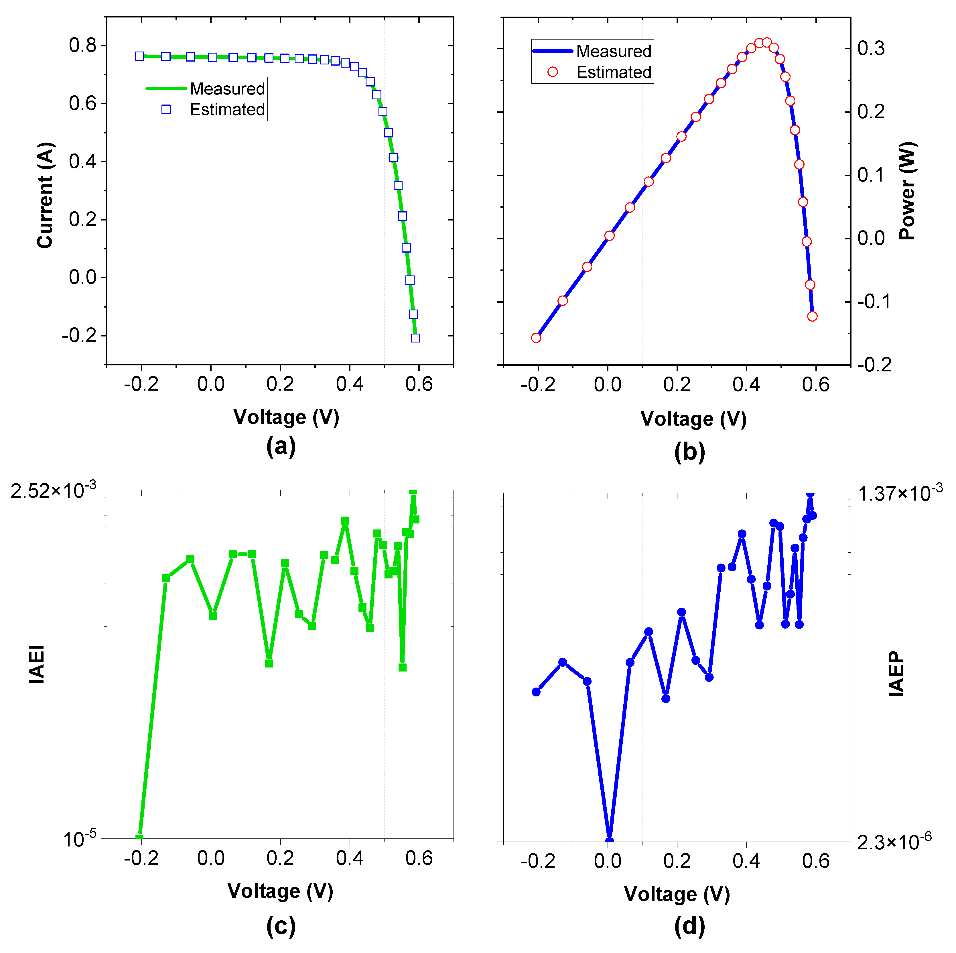
Figure 7.
Estimated and measured data of the RTC France silicon solar cell based on DDM by ICO; (a) I–V, (b) P–V, (c) IAEI, and (d) IAEP.
Figure 7.
Estimated and measured data of the RTC France silicon solar cell based on DDM by ICO; (a) I–V, (b) P–V, (c) IAEI, and (d) IAEP.
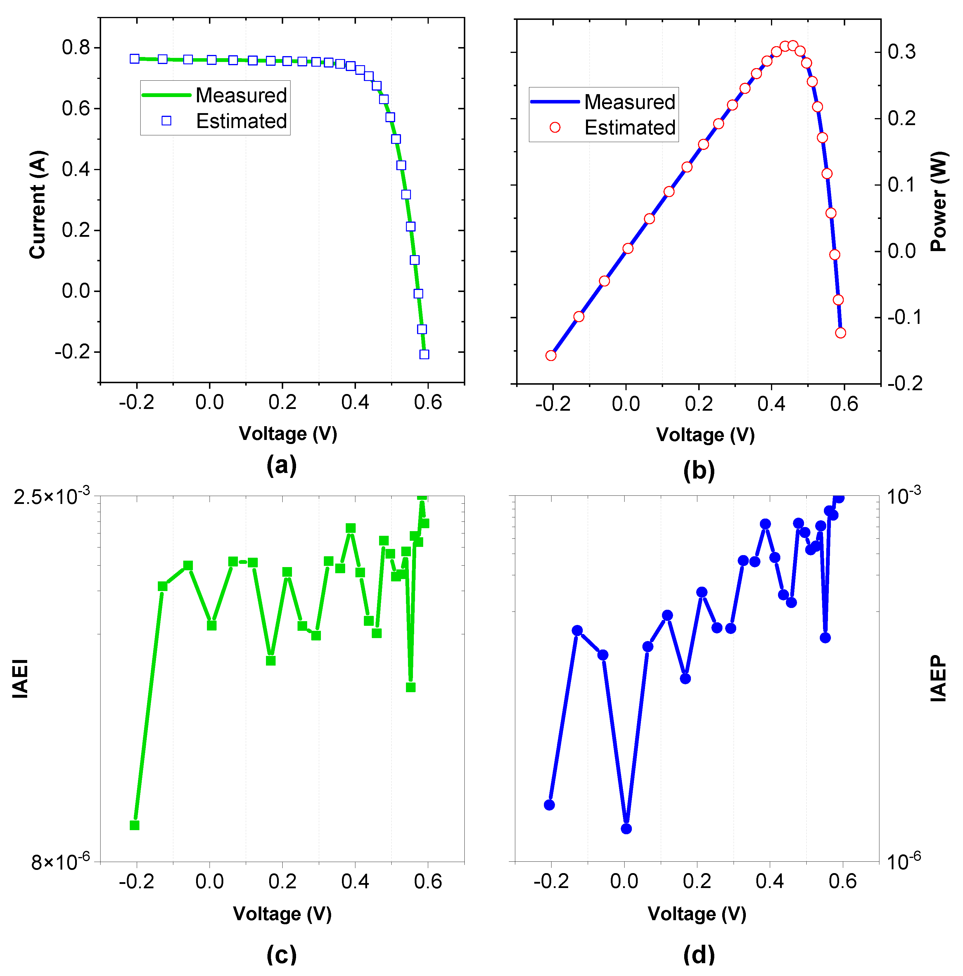
Figure 8.
Estimated and measured data yielded by ICO for the PV module model based on Photo Watt-PWP 201; (a) I–V, (b) P–V, (c) IAEI, and (d) IAEP.
Figure 8.
Estimated and measured data yielded by ICO for the PV module model based on Photo Watt-PWP 201; (a) I–V, (b) P–V, (c) IAEI, and (d) IAEP.
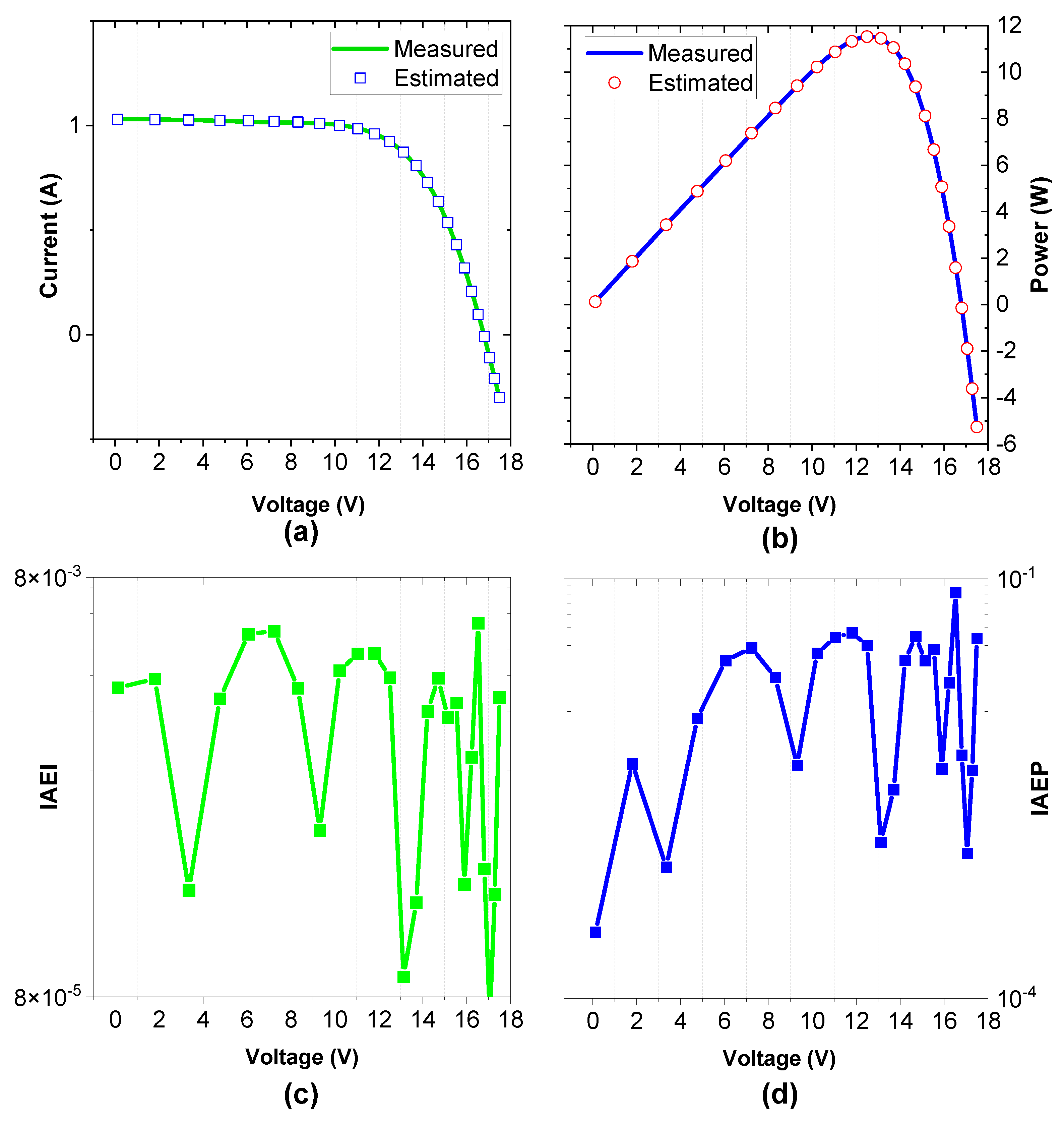
Figure 9.
Final ranking of applied algorithms for three models based on the Friedman test: (a) n = 40, and (b) n = 80.
Figure 9.
Final ranking of applied algorithms for three models based on the Friedman test: (a) n = 40, and (b) n = 80.
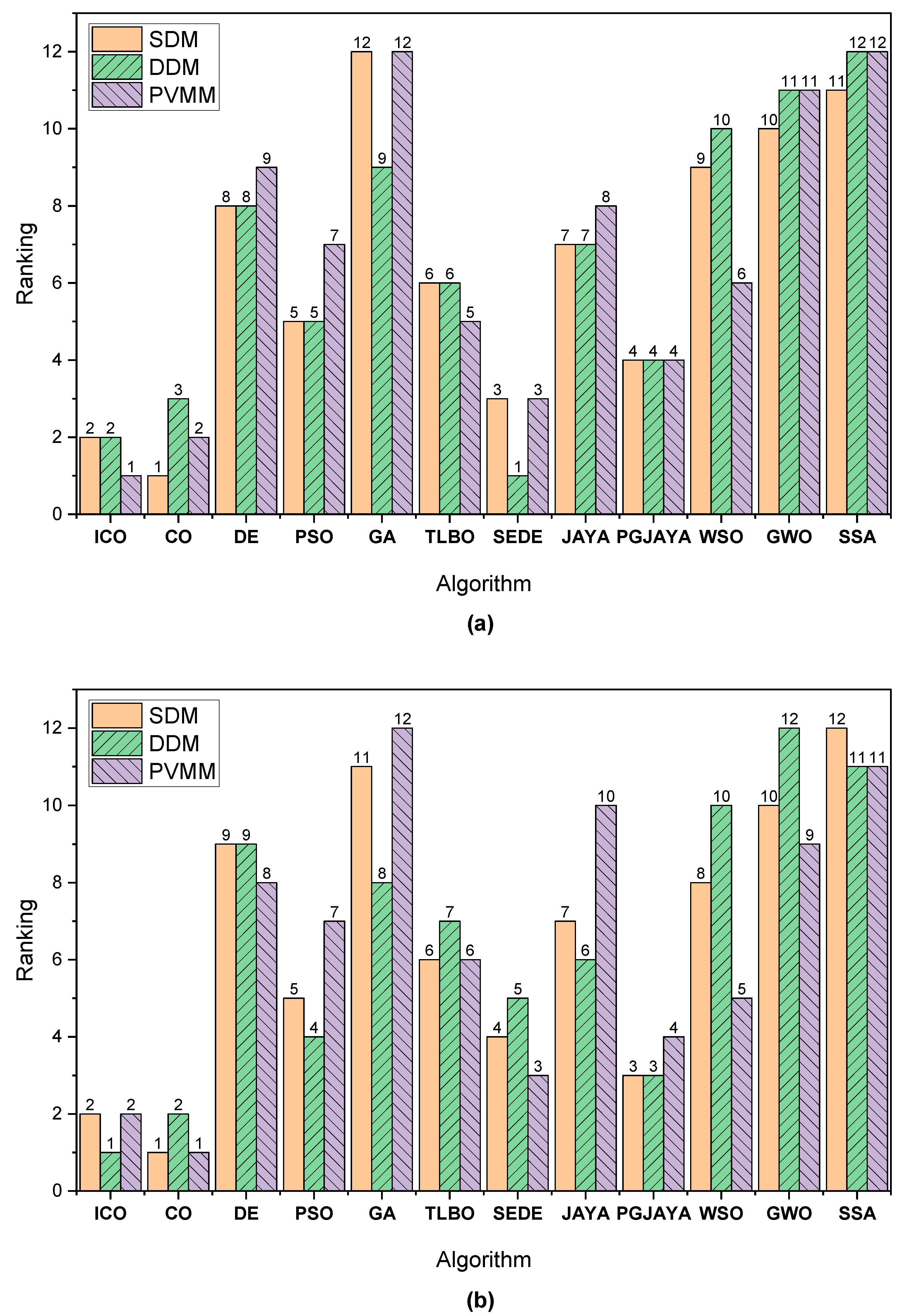
Figure 10.
Boxplot of best RMSE in 30 runs for n = 40: (a) SDM, (b) DDM, and (c) PVMM.
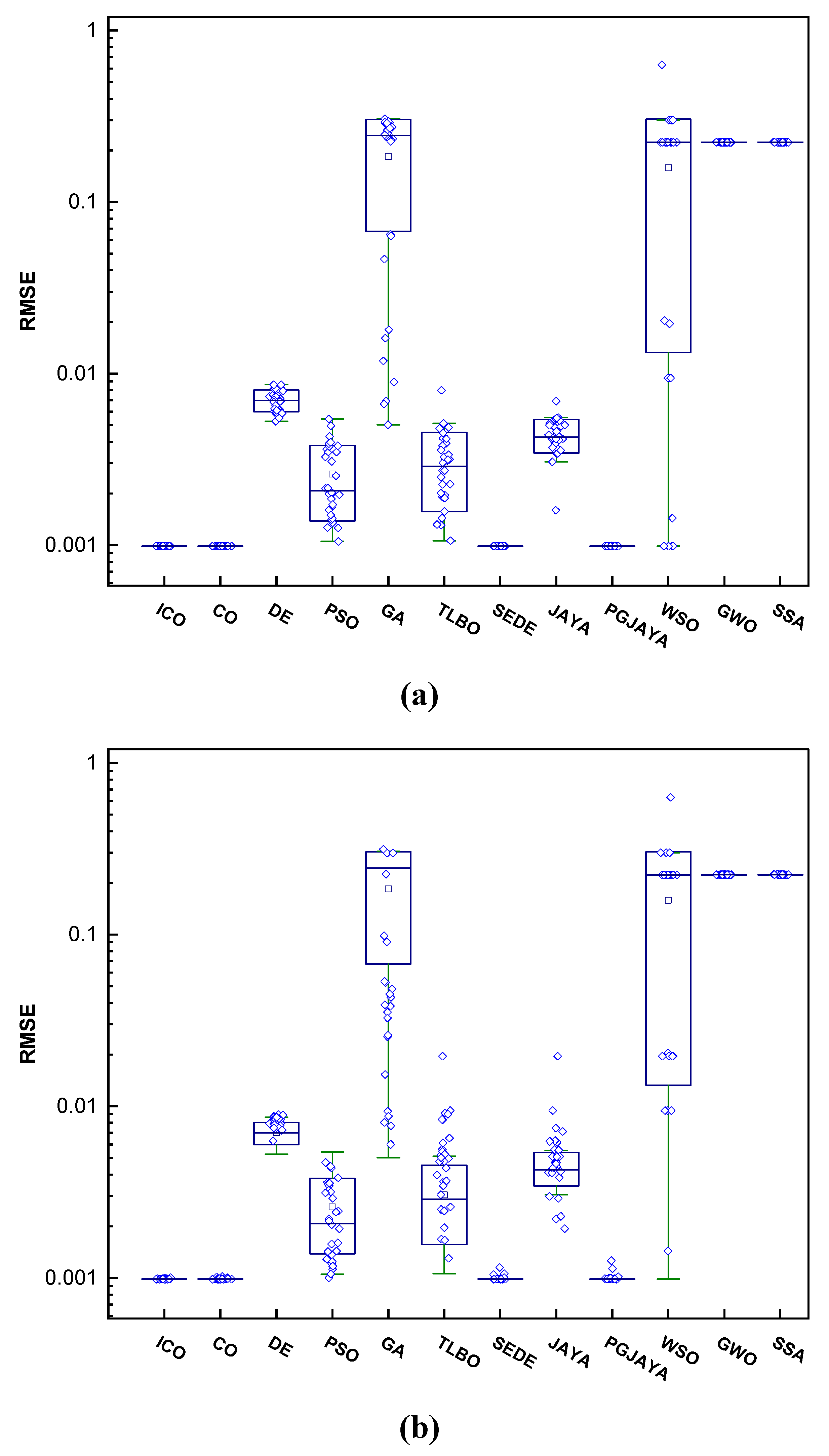
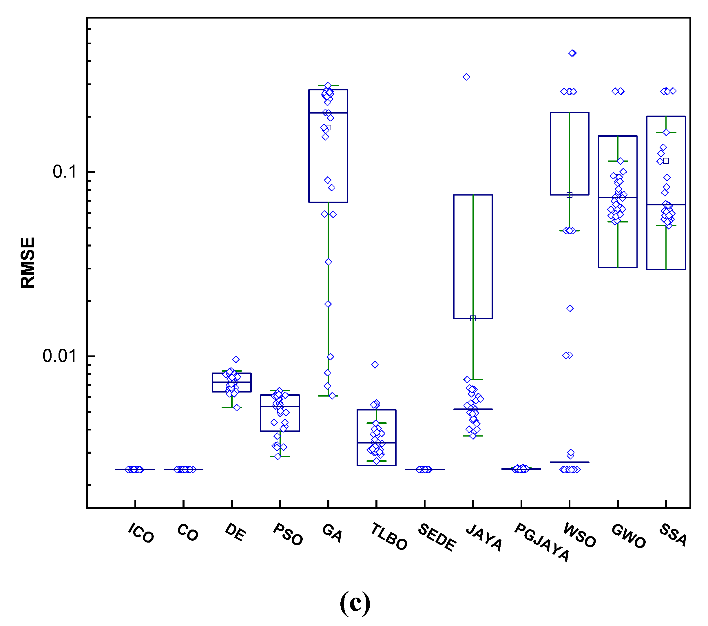
Figure 11.
CPU time over 30 runs by different algorithms with n = 40 for SDM, DDM, and PVMM.
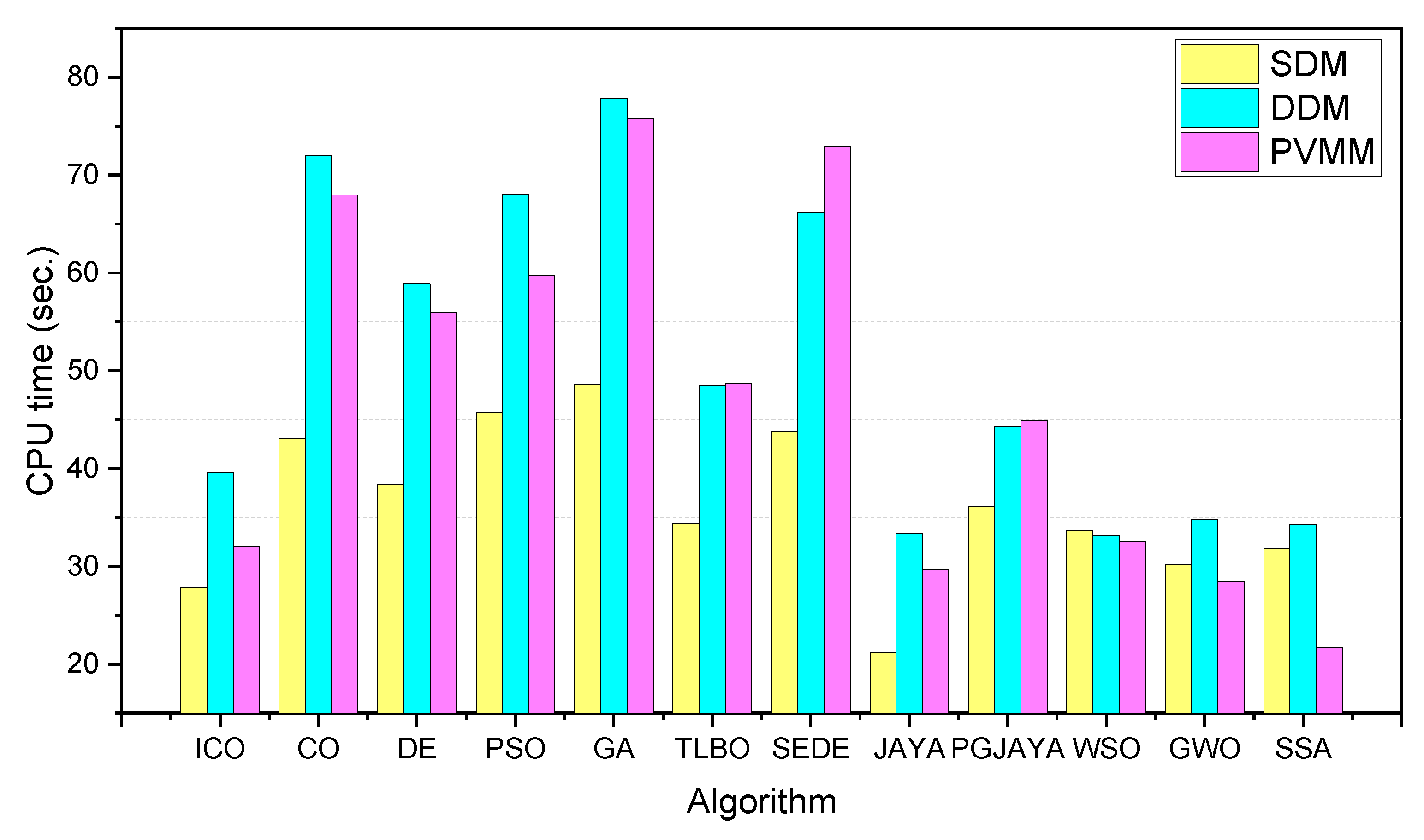
Figure 12.
Convergence curves of comparative algorithms with n = 40 for three models; (a) SDM, (b) DDM, and (c) PVMM.
Figure 12.
Convergence curves of comparative algorithms with n = 40 for three models; (a) SDM, (b) DDM, and (c) PVMM.
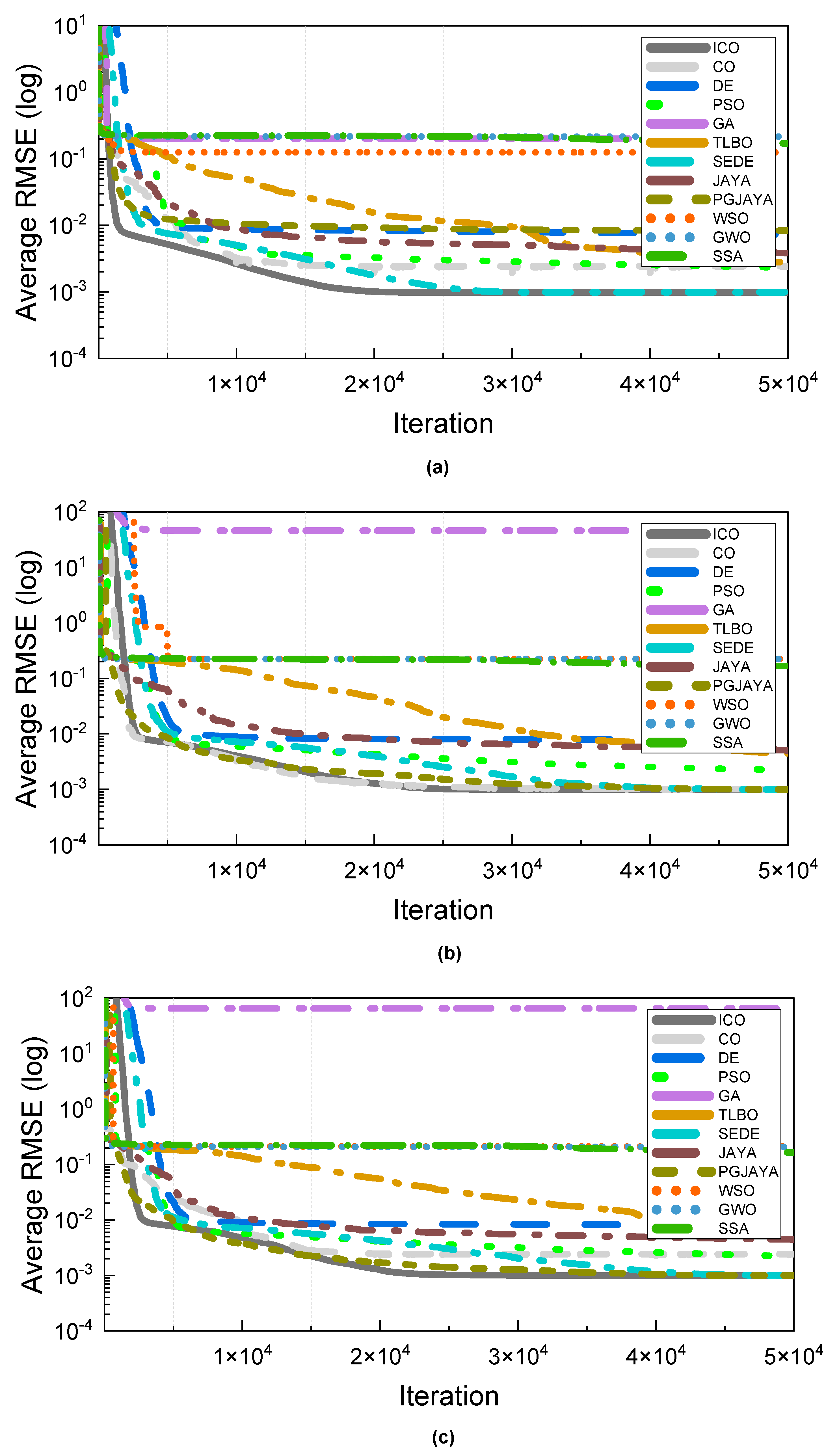
Figure 13.
Exploration-exploration and diversity of comparative algorithms on SDM.
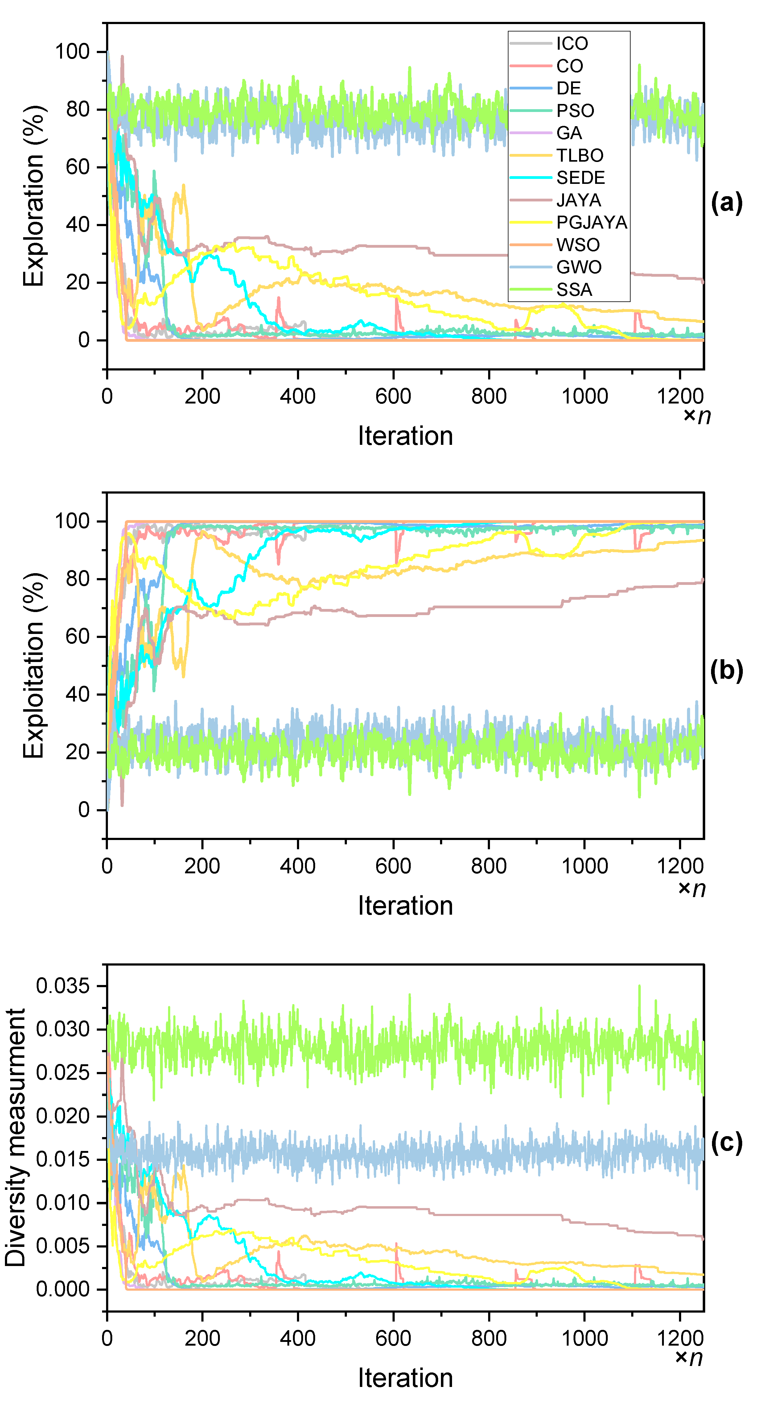
Figure 14.
Mean Exploration-exploitation of comparative algorithms on SDM.
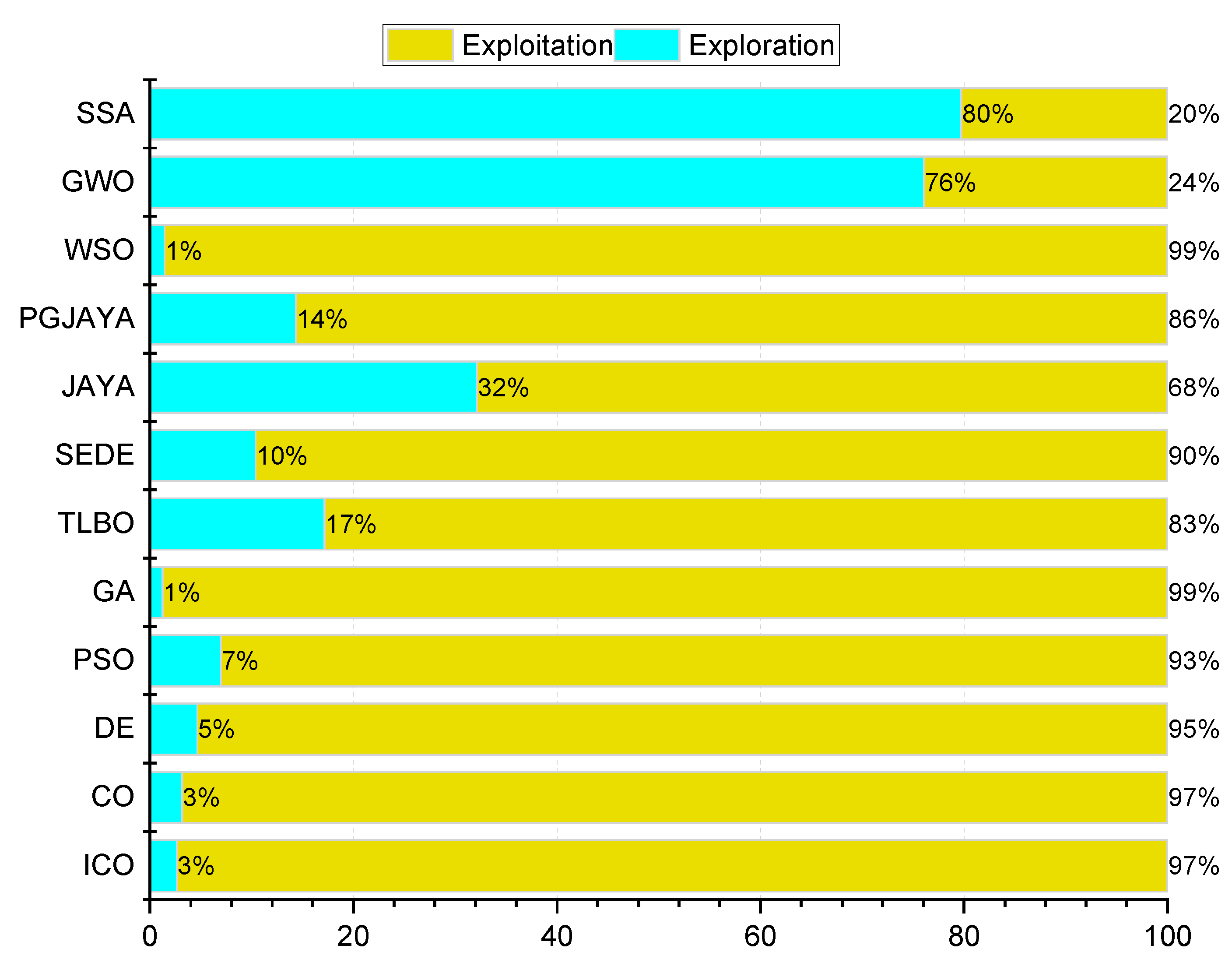

Table 1.
A review of the solar PV parameter extraction methods.
| Algorithm | PV Type | PV Model | Disadvantage | Advantage |
|---|---|---|---|---|
| PGJAYA [1] | RTC France Si cell and PhotoWatt-PWP201 | SDM, DDM, PVMM | Insufficient reliability | Acceptable accuracy |
| DE [2] | SM55 Module | SDM | The parameters need to be adjusted, insufficient capability for exploitation. | Accurate performance under a variety of operating conditionsPossessing good exploration capabilities |
| PSO [3] | Not specified | SDM, DDM | Stuck in local minima, convergence at the beginning | High level of accuracy in the solutionEase of implementationRobustness |
| SEDE [4] | RTC France Si cell and PhotoWatt-PWP201 | SDM, DDM, PVMM | High computation time | High accuracy and robustness |
| WSO [5] | RTC France silicon solar cell, Photo watt-PWP 201, and STM6-40/36 PV modules | SDM, DDM, PVMM | Insufficient robustness | New optimization algorithm for parameter extraction of PV cells and modules, low CPU time |
| SSA [6] | TITAN-12-50 | DDM | Caught within local minimums, convergence occurs early in the process | Low computational time |
| IJAYA [7] | RTC France Si cell | SDM, DDM | Caught by local minima, Inaccurate solution | A simpler and more efficient algorithmConvergence and robustness are high |
| Rao [8] | RTC France Si cell and PhotoWatt-PWP201 | SDM, DDM | Stuck in local minima, commercial modules haven’t been tested | Ease of implementationThe ability to explore well |
| MABC [9] | RTC France Si cell | SDM, DDM | Excessive computation timeParameters need to be adjusted frequently, achieving convergence early | High accuracy and robustnessInsensitive to noise |
| IMFO [10] | Q6-1380 solar cell and CS6P-240P module | SDM, DDM | It takes a long time to compute, commercial modules have not been tested | Convergence speed is high, it is simpler |
| SFLA [11] | KC200GT and MSX-60 | SDM | Not accurateA lot of control parameters | Fast convergence |
| TPTLBO [12] | RTC France Si cell | SDM, DDM | High computational costsUncertainty about the solution | Ease of implementationFewer control parametersFast convergence |
| ICWO [13] | KC200GT | SDM, DDM | Inability to explore, caught within local minimums, convergence occurs early in the process | Easily implemented, a lower cost of computationCapacity for fair exploitation |
| SCA [14] | KC200GT | SDM | KC200GT module only tested, a local minimum trap | Easy to implement and simple to use, a fair degree of accuracy |
| GWO-CS [15] | KC200GT | SDM | The convergence speed is very slow | A robust designReduced possibility of local optima trappingThe accuracy of the solution is high |
| COA [16] | RTC France Si cell, PhotoWatt-PWP201, KC200GT, ST40, and SM55 | SDM, DDM | Insufficient ability to exploit, convergence at an early stage | The quality of the solution is high, high convergence speed |
| MPA [17] | KC200GT and MSX-60 | DDM | Convergence at an early stageStuck in local minima | A high degree of accuracy in the solutionExcel exploratory skills |
| AGA [18] | RTC France Si cell | SDM | Caught in the trap of local minima, a lack of local search capability | A reasonable degree of accuracyIdentify promising search areas to find solutions |
| IEO [19] | RTC France Si cell, PhotoWatt-PWP201, ST40, and SM55 | SDM, DDM | Long computation times | High level of accuracyA good ability to explore and exploit |
| SMA [20] | RTC France Si cell and PhotoWatt-PWP201 | SDM, DDM | It takes a long time to compute | A high degree of accuracy, a good ability to explore and exploit |
| OAHHO [21] | RTC France Si cell, PhotoWatt-PWP201, PVM 752 GaAs, ST40, and SM55 | SDM, DDM | Not specified | Rapid convergence ratesAvoiding local optimum situationsHigh-quality solutions |
Table 2.
Parameters’ bounds for three models.
| Model | |||||||||||||||
|---|---|---|---|---|---|---|---|---|---|---|---|---|---|---|---|
| Min | Max | Min | Max | Min | Max | Min | Max | Min | Max | ||||||
| SDM | 0 | 1 | 0 | 1 | 1 | 2 | 0 | 0.5 | 0 | 100 | |||||
| DDM | 0 | 1 | 0 | 1 | 1 | 2 | 0 | 0.5 | 0 | 100 | |||||
| PV module | 0 | 2 | 0 | 50 | 1 | 50 | 0 | 2 | 0 | 2000 | |||||
Table 3.
An analysis of the effect of population size on ICO performance for different PV models.
| Model | n | Min | Mean | Max | SD | CPU time (sec.) | Mean rank in the Freidman test | Sum rank in the Freidman test |
|---|---|---|---|---|---|---|---|---|
| SD | 10 | 9.860219E-04 | 1.006557E-03 | 1.268819E-03 | 5.47E-05 | 48.59 | 6.0 | 180 |
| 20 | 9.860219E-04 | 9.860219E-04 | 9.860219E-04 | 8.17E-17 | 48.02 | 3.6 | 106.5 | |
| 40 | 9.860219E-04 | 9.860219E-04 | 9.860219E-04 | 6.30E-17 | 37.42 | 2.6 | 76.5 | |
| 50 | 9.860219E-04 | 9.860219E-04 | 9.860219E-04 | 3.24E-17 | 40.23 | 2.5 | 74.5 | |
| 80 | 9.860219E-04 | 9.860219E-04 | 9.860219E-04 | 4.85E-17 | 41.11 | 2.9 | 87 | |
| 100 | 9.860219E-04 | 9.860219E-04 | 9.860219E-04 | 4.66E-17 | 50.89 | 3.5 | 105.5 | |
| DD | 10 | 9.849747E-04 | 1.046876E-03 | 1.199696E-03 | 5.90E-05 | 52.52 | 5.6 | 169 |
| 20 | 9.832470E-04 | 9.909079E-04 | 1.016172E-03 | 8.43E-06 | 55.21 | 3.9 | 116 | |
| 40 | 9.824888E-04 | 9.869534E-04 | 1.002805E-03 | 4.35E-06 | 53.12 | 2.9 | 87 | |
| 50 | 9.825601E-04 | 9.861925E-04 | 9.948859E-04 | 2.43E-06 | 50.93 | 3.0 | 90 | |
| 80 | 9.824849E-04 | 9.860955E-04 | 9.895027E-04 | 1.43E-06 | 38.32 | 2.6 | 78 | |
| 100 | 9.836909E-04 | 9.878873E-04 | 1.014303E-03 | 6.14E-06 | 36.53 | 3.0 | 90 | |
| PVM | 10 | 2.425075E-03 | 2.435752E-03 | 2.498069E-03 | 1.99E-05 | 48.36 | 6.0 | 180 |
| 20 | 2.425075E-03 | 2.425075E-03 | 2.425075E-03 | 2.14E-16 | 44.27 | 4.1 | 124 | |
| 40 | 2.425075E-03 | 2.425075E-03 | 2.425075E-03 | 1.24E-16 | 46.07 | 2.7 | 81 | |
| 50 | 2.425075E-03 | 2.425075E-03 | 2.425075E-03 | 3.65E-17 | 44.76 | 2.8 | 84.5 | |
| 80 | 2.425075E-03 | 2.425075E-03 | 2.425075E-03 | 2.65E-17 | 39.16 | 2.5 | 75 | |
| 100 | 2.425075E-03 | 2.425075E-03 | 2.425075E-03 | 3.17E-17 | 39.84 | 2.9 | 85.5 |
Table 4.
Optimal parameters of SDM obtained by different algorithms with n = 40.
| n | Algorithm | RMSE | |||||
|---|---|---|---|---|---|---|---|
| 40 | ICO | 0.761 | 3.23E-07 | 53.719 | 0.0364 | 1.4812 | 9.860218778914E-04 |
| CO | 0.761 | 3.23E-07 | 53.719 | 0.0364 | 1.4812 | 9.860218778914E-04 | |
| DE | 0.763 | 3.18E-06 | 100.000 | 0.0243 | 1.7547 | 5.274028415510E-03 | |
| PSO | 0.761 | 2.67E-07 | 48.768 | 0.0371 | 1.4623 | 1.049908843005E-03 | |
| GA | 0.764 | 2.63E-06 | 70.532 | 0.0257 | 1.7285 | 5.028715197625E-03 | |
| TLBO | 0.761 | 3.77E-07 | 63.546 | 0.0358 | 1.4967 | 1.061394487359E-03 | |
| SEDE | 0.761 | 3.23E-07 | 53.719 | 0.0364 | 1.4812 | 9.860218778915E-04 | |
| JAYA | 0.761 | 6.08E-07 | 70.138 | 0.0337 | 1.5478 | 1.596303286167E-03 | |
| PGJAYA | 0.761 | 3.23E-07 | 53.713 | 0.0364 | 1.4812 | 9.860219332331E-04 | |
| WSO | 0.761 | 3.23E-07 | 53.719 | 0.0364 | 1.4812 | 9.860218778915E-04 | |
| GWO | 0.838 | 0.00E+00 | 1.139 | 0.0000 | 2.0000 | 2.228699161204E-01 | |
| SSA | 0.835 | 0.00E+00 | 1.162 | 0.0000 | 1.0000 | 2.228762271791E-01 | |
| 80 | ICO | 0.761 | 3.23E-07 | 53.719 | 0.0364 | 1.4812 | 9.860218778914E-04 |
| CO | 0.761 | 3.23E-07 | 53.719 | 0.0364 | 1.4812 | 9.860218778914E-04 | |
| DE | 0.763 | 1.54E-06 | 99.600 | 0.0296 | 1.6569 | 3.541687987531E-03 | |
| PSO | 0.761 | 3.54E-07 | 56.556 | 0.0360 | 1.4903 | 1.001530647734E-03 | |
| GA | 0.759 | 1.29E-07 | 46.427 | 0.0399 | 1.3938 | 2.248309383635E-03 | |
| TLBO | 0.761 | 3.40E-07 | 55.608 | 0.0362 | 1.4865 | 9.917684200620E-04 | |
| SEDE | 0.761 | 3.36E-07 | 54.054 | 0.0362 | 1.4852 | 9.902825250634E-04 | |
| JAYA | 0.762 | 9.73E-07 | 88.523 | 0.0312 | 1.6013 | 2.589835639165E-03 | |
| PGJAYA | 0.761 | 3.23E-07 | 53.722 | 0.0364 | 1.4812 | 9.860220454267E-04 | |
| WSO | 0.761 | 3.23E-07 | 53.719 | 0.0364 | 1.4812 | 9.860218778915E-04 | |
| GWO | 0.769 | 4.43E-06 | 24.455 | 0.0200 | 1.8059 | 9.281563258264E-03 | |
| SSA | 1.000 | 8.72E-07 | 1.098 | 0.0007 | 1.6512 | 1.525312427660E-01 |
Table 5.
Optimal parameters for DDM obtained by different algorithms with n = 40.
| n | Algorithm | RMSE | |||||||
|---|---|---|---|---|---|---|---|---|---|
| 40 | ICO | 0.760781 | 7.46E-07 | 2.26E-07 | 0.036740 | 55.456 | 2.000 | 1.4511 | 9.82486099138E-04 |
| CO | 0.760781 | 7.50E-07 | 2.26E-07 | 0.036741 | 55.486 | 2.000 | 1.4510 | 9.82484882272E-04 | |
| DE | 0.764966 | 2.55E-06 | 2.40E-06 | 0.022457 | 100.000 | 1.752 | 1.9806 | 6.28139269321E-03 | |
| PSO | 0.760733 | 1.71E-07 | 1.46E-06 | 0.036757 | 61.054 | 1.429 | 2.0000 | 1.00247341473E-03 | |
| GA | 0.763271 | 0.00E+00 | 4.23E-06 | 0.022775 | 97.844 | 1.670 | 1.7963 | 5.99279194424E-03 | |
| TLBO | 0.760090 | 9.73E-08 | 2.76E-06 | 0.036975 | 100.000 | 1.387 | 1.9994 | 1.30300020067E-03 | |
| SEDE | 0.760769 | 2.14E-07 | 8.07E-07 | 0.036790 | 55.795 | 1.447 | 1.9869 | 9.82753663536E-04 | |
| JAYA | 0.759873 | 5.29E-07 | 4.02E-11 | 0.034438 | 70.729 | 1.532 | 1.8894 | 1.93867560984E-03 | |
| PGJAYA | 0.760782 | 2.45E-07 | 2.90E-07 | 0.036477 | 54.289 | 1.999 | 1.4720 | 9.84193519571E-04 | |
| WSO | 0.759500 | 4.52E-07 | 0.00E+00 | 0.035285 | 100.000 | 1.516 | 2.0000 | 1.43847589737E-03 | |
| GWO | 1.000000 | 0.00E+00 | 1.16E-05 | 0.000000 | 2.179 | 1.000 | 2.0000 | 1.54903625180E-01 | |
| SSA | 0.834308 | 0.00E+00 | 0.00E+00 | 0.000000 | 1.152 | 1.000 | 1.0000 | 2.22868413284E-01 | |
| 80 | ICO | 0.760780 | 6.63E-07 | 2.36E-07 | 0.036695 | 55.257 | 2.000 | 1.4547 | 9.82538943274E-04 |
| CO | 0.760781 | 2.22E-07 | 7.72E-07 | 0.036757 | 55.539 | 1.450 | 1.9969 | 9.82528425982E-04 | |
| DE | 0.763865 | 5.19E-08 | 9.13E-06 | 0.023974 | 99.963 | 1.407 | 1.9937 | 6.73013079580E-03 | |
| PSO | 0.760797 | 6.03E-07 | 2.03E-07 | 0.036852 | 54.797 | 1.900 | 1.4430 | 9.84648707354E-04 | |
| GA | 0.760727 | 0.00E+00 | 9.74E-07 | 0.031507 | 100.000 | 1.681 | 1.6015 | 2.39573932360E-03 | |
| TLBO | 0.760754 | 3.22E-07 | 5.04E-17 | 0.036453 | 55.423 | 1.481 | 1.0230 | 9.95677091382E-04 | |
| SEDE | 0.760178 | 8.63E-07 | 2.07E-07 | 0.034961 | 82.980 | 1.806 | 1.4577 | 1.47037750973E-03 | |
| JAYA | 0.761997 | 1.39E-06 | 0.00E+00 | 0.028824 | 100.000 | 1.644 | 2.0000 | 3.57709882707E-03 | |
| PGJAYA | 0.760851 | 5.18E-07 | 2.30E-07 | 0.036667 | 54.633 | 1.917 | 1.4533 | 9.84200147988E-04 | |
| WSO | 0.760776 | 0.00E+00 | 3.23E-07 | 0.036377 | 53.719 | 2.000 | 1.4812 | 9.86021877892E-04 | |
| GWO | 0.999003 | 0.00E+00 | 5.29E-06 | 0.000514 | 1.373 | 2.000 | 1.8772 | 1.38743574369E-01 | |
| SSA | 0.836762 | 1.17E-09 | 0.00E+00 | 0.000071 | 1.149 | 1.121 | 1.4507 | 1.57126305055E-01 |
Table 6.
Optimal parameters for PVMM by different algorithms with n = 40 and n = 80.
| n | Algorithm | RMSE | |||||
|---|---|---|---|---|---|---|---|
| 40 | ICO | 1.03051 | 3.48E-06 | 27.277 | 0.0334 | 1.3512 | 2.425074868095030E-03 |
| CO | 1.03051 | 3.48E-06 | 27.277 | 0.0334 | 1.3512 | 2.425074868094980E-03 | |
| DE | 1.02991 | 1.49E-05 | 1065.617 | 0.0284 | 1.5261 | 5.266650305240960E-03 | |
| PSO | 1.02677 | 5.98E-06 | 88.261 | 0.0318 | 1.4111 | 2.864391667859010E-03 | |
| GA | 1.02370 | 1.52E-05 | 1944.805 | 0.0278 | 1.5294 | 6.099240455880790E-03 | |
| TLBO | 1.02611 | 4.78E-06 | 75.270 | 0.0325 | 1.3855 | 2.700403640152360E-03 | |
| SEDE | 1.03051 | 3.48E-06 | 27.277 | 0.0334 | 1.3512 | 2.425074868095090E-03 | |
| JAYA | 1.02742 | 8.89E-06 | 911.208 | 0.0305 | 1.4586 | 3.697656950234140E-03 | |
| PGJAYA | 1.03052 | 3.48E-06 | 27.250 | 0.0334 | 1.3511 | 2.425077305006140E-03 | |
| WSO | 1.03051 | 3.48E-06 | 27.277 | 0.0334 | 1.3512 | 2.425074868095050E-03 | |
| GWO | 1.04843 | 5.00E-05 | 3.016 | 0.0000 | 1.7509 | 5.383466416567090E-02 | |
| SSA | 1.15116 | 5.00E-05 | 2.191 | 0.0129 | 1.7224 | 5.130174319081860E-02 | |
| 80 | ICO | 1.03051 | 3.48E-06 | 27.277 | 0.0334 | 1.3512 | 2.425074868095010E-03 |
| CO | 1.03051 | 3.48E-06 | 27.277 | 0.0334 | 1.3512 | 2.425074868094990E-03 | |
| DE | 1.02868 | 2.27E-05 | 1968.622 | 0.0264 | 1.5866 | 6.921126739647050E-03 | |
| PSO | 1.02664 | 6.66E-06 | 115.721 | 0.0314 | 1.4238 | 3.029451135597340E-03 | |
| GA | 1.03138 | 2.87E-05 | 2000.000 | 0.0252 | 1.6215 | 7.712963596737400E-03 | |
| TLBO | 1.02522 | 5.63E-06 | 881.405 | 0.0321 | 1.4034 | 3.244452302450550E-03 | |
| SEDE | 1.03013 | 3.56E-06 | 28.820 | 0.0333 | 1.3536 | 2.427164258722220E-03 | |
| JAYA | 1.02758 | 1.51E-05 | 1713.306 | 0.0277 | 1.5278 | 5.590302366807740E-03 | |
| PGJAYA | 1.02922 | 4.29E-06 | 33.745 | 0.0327 | 1.3739 | 2.518017787843970E-03 | |
| WSO | 1.03051 | 3.48E-06 | 27.277 | 0.0334 | 1.3512 | 2.425074868095060E-03 | |
| GWO | 1.07157 | 5.00E-05 | 5.528 | 0.0187 | 1.7213 | 2.019064583084870E-02 | |
| SSA | 1.06056 | 4.31E-05 | 12.652 | 0.0238 | 1.6888 | 1.554532543514840E-02 |
Table 7.
Statistical results of different algorithms with n = 40 and n = 80 for SDM.
| n | Algorithm | Min | Mean | Max | SD | Mean rank | Sum rank | Significance |
|---|---|---|---|---|---|---|---|---|
| 40 | ICO | 9.86021877891E-04 | 9.86021877892E-04 | 9.86021877892E-04 | 3.091E-17 | 1.633 | 49 | |
| CO | 9.86021877891E-04 | 9.86021877892E-04 | 9.86021877893E-04 | 2.299E-16 | 1.600 | 48 | ||
| DE | 5.27402841551E-03 | 7.00472269280E-03 | 8.61400240318E-03 | 1.008E-03 | 8.200 | 246 | ||
| PSO | 1.04990884301E-03 | 2.59824261345E-03 | 5.43861383375E-03 | 1.215E-03 | 5.700 | 171 | ||
| GA | 5.02871519763E-03 | 1.85106717646E-01 | 3.05981702986E-01 | 1.178E-01 | 10.933 | 328 | ||
| TLBO | 1.06139448736E-03 | 3.05558085709E-03 | 7.98832352445E-03 | 1.489E-03 | 5.867 | 176 | ||
| SEDE | 9.86021877891E-04 | 9.86021877892E-04 | 9.86021877892E-04 | 4.368E-17 | 2.867 | 86 | ||
| JAYA | 1.59630328617E-03 | 4.42292722271E-03 | 6.90548939964E-03 | 9.777E-04 | 6.933 | 208 | ||
| PGJAYA | 9.86021933233E-04 | 9.86276195755E-04 | 9.89060476576E-04 | 6.385E-07 | 4.133 | 124 | ||
| WSO | 9.86021877892E-04 | 1.58438200609E-01 | 6.30741696212E-01 | 1.452E-01 | 8.733 | 262 | ||
| GWO | 2.22869916120E-01 | 2.23053219785E-01 | 2.23414777753E-01 | 1.541E-04 | 10.600 | 318 | ||
| SSA | 2.22876227179E-01 | 2.23093108473E-01 | 2.23798438512E-01 | 1.976E-04 | 10.800 | 324 | ||
| 80 | ICO | 9.86021877891E-04 | 9.86021877892E-04 | 9.86021877892E-04 | 5.21E-17 | 1.933 | 58 | |
| CO | 9.86021877891E-04 | 9.86021877891E-04 | 9.86021877892E-04 | 1.02E-16 | 1.267 | 38 | ||
| DE | 3.54168798753E-03 | 7.44468352091E-03 | 8.66642059402E-03 | 8.63E-04 | 8.233 | 247 | ||
| PSO | 1.00153064773E-03 | 2.60127712828E-03 | 4.82228315158E-03 | 1.30E-03 | 5.633 | 169 | ||
| GA | 2.24830938364E-03 | 1.73964495048E-01 | 2.97093810571E-01 | 9.96E-02 | 10.767 | 323 | ||
| TLBO | 9.91768420062E-04 | 5.34155103461E-03 | 1.97944235719E-02 | 4.83E-03 | 6.600 | 198 | ||
| SEDE | 9.90282525063E-04 | 1.01400153629E-03 | 1.09363977975E-03 | 2.20E-05 | 4.033 | 121 | ||
| JAYA | 2.58983563916E-03 | 5.68192621557E-03 | 9.00499477318E-03 | 1.14E-03 | 7.067 | 212 | ||
| PGJAYA | 9.86022045427E-04 | 1.01574698584E-03 | 1.18949290801E-03 | 4.93E-05 | 3.767 | 113 | ||
| WSO | 9.86021877892E-04 | 3.86485383212E-02 | 2.99953326338E-01 | 8.23E-02 | 7.233 | 217 | ||
| GWO | 9.28156325826E-03 | 2.08662190383E-01 | 2.22887009586E-01 | 5.41E-02 | 10.650 | 319.5 | ||
| SSA | 1.52531242766E-01 | 1.76192424924E-01 | 2.22861399093E-01 | 2.22E-02 | 10.817 | 324.5 |
Table 8.
Statistical results of different algorithms with n = 40 and n = 80 for DDM.
| n | Algorithm | Min | Mean | Max | SD | Mean rank | Sum rank | Sign. |
| 40 | ICO | 9.82486099138221E-04 | 9.87266271841069E-04 | 1.00565345910251E-03 | 5.0E-06 | 2.400 | 72 | |
| CO | 9.82484882272263E-04 | 9.90014277022917E-04 | 1.02092378170200E-03 | 9.2E-06 | 2.667 | 80 | ||
| DE | 6.28139269320691E-03 | 8.08813241671442E-03 | 8.93742409284825E-03 | 5.8E-04 | 7.867 | 236 | ||
| PSO | 1.00247341473318E-03 | 2.42462675866429E-03 | 4.70972999662043E-03 | 1.2E-03 | 5.233 | 157 | ||
| GA | 5.99279194423828E-03 | 9.40346251766308E-02 | 3.14531449266952E-01 | 9.2E-02 | 9.533 | 286 | ||
| TLBO | 1.30300020066498E-03 | 5.31395638216597E-03 | 1.95451852804007E-02 | 3.5E-03 | 6.533 | 196 | ||
| SEDE | 9.82753663536365E-04 | 9.96916197397831E-04 | 1.15176160603947E-03 | 3.4E-05 | 2.133 | 64 | ||
| JAYA | 1.93867560984064E-03 | 5.30491570084624E-03 | 1.95452348011886E-02 | 3.1E-03 | 6.567 | 197 | ||
| PGJAYA | 9.84193519571165E-04 | 1.00336927015568E-03 | 1.26370280495224E-03 | 5.6E-05 | 2.867 | 86 | ||
| WSO | 1.43847589736749E-03 | 1.86584575264940E-01 | 6.30741696211904E-01 | 1.5E-01 | 9.967 | 299 | ||
| GWO | 1.54903625179668E-01 | 2.21100841293962E-01 | 2.24562995128955E-01 | 1.3E-02 | 11.067 | 332 | ||
| SSA | 2.22868413284217E-01 | 2.23443763002107E-01 | 2.24750772827690E-01 | 5.3E-04 | 11.167 | 335 | ||
| 80 | ICO | 9.8253894327E-04 | 9.8641995737E-04 | 9.9981923040E-04 | 3.134E-06 | 1.633 | 49 | |
| CO | 9.8252842598E-04 | 9.9825780367E-04 | 1.0827441957E-03 | 2.432E-05 | 1.900 | 57 | ||
| DE | 6.7301307958E-03 | 8.0618449324E-03 | 8.8108931833E-03 | 6.169E-04 | 7.933 | 238 | ||
| PSO | 9.8464870735E-04 | 2.3813391278E-03 | 5.5055357165E-03 | 1.184E-03 | 4.533 | 136 | ||
| GA | 2.3957393236E-03 | 2.2114853037E-02 | 1.1924927342E-01 | 3.269E-02 | 7.800 | 234 | ||
| TLBO | 9.9567709138E-04 | 1.8966303725E-02 | 6.2679374194E-02 | 1.887E-02 | 7.700 | 231 | ||
| SEDE | 1.4703775097E-03 | 2.6141249460E-03 | 4.0397037616E-03 | 8.191E-04 | 4.833 | 145 | ||
| JAYA | 3.5770988271E-03 | 6.7480847825E-03 | 9.7931015684E-03 | 1.726E-03 | 7.067 | 212 | ||
| PGJAYA | 9.8420014799E-04 | 1.0315913230E-03 | 1.3731176270E-03 | 7.747E-05 | 2.700 | 81 | ||
| WSO | 9.8602187789E-04 | 1.1327669684E-01 | 2.9995332634E-01 | 1.185E-01 | 9.700 | 291 | ||
| GWO | 1.3874357437E-01 | 1.6797247572E-01 | 2.2219565068E-01 | 1.317E-02 | 11.167 | 335 | ||
| SSA | 1.5712630505E-01 | 1.6563118085E-01 | 1.7878158052E-01 | 5.962E-03 | 11.033 | 331 |
Table 9.
Statistical results of different algorithms with n = 40 and n = 80 for PVMM.
| n | Algorithm | Min | Mean | Max | SD | Mean rank | Sum rank | Sign. |
|---|---|---|---|---|---|---|---|---|
| 40 | ICO | 2.4250748680950E-03 | 2.4250748680950E-03 | 2.4250748680950E-03 | 4.998E-17 | 1.917 | 57.5 | |
| CO | 2.4250748680950E-03 | 2.4250748680950E-03 | 2.4250748680950E-03 | 1.105E-16 | 1.983 | 59.5 | ||
| DE | 5.2666503052410E-03 | 7.2566226992670E-03 | 9.6379708296680E-03 | 8.375E-04 | 8.433 | 253 | ||
| PSO | 2.8643916678590E-03 | 5.0462723254080E-03 | 6.5034717549490E-03 | 1.123E-03 | 6.800 | 204 | ||
| GA | 6.0992404558810E-03 | 1.7462237365350E-01 | 2.9547389242870E-01 | 1.059E-01 | 11.000 | 330 | ||
| TLBO | 2.7004036401520E-03 | 3.8363781147850E-03 | 9.0053151975850E-03 | 1.277E-03 | 5.933 | 178 | ||
| SEDE | 2.4250748680950E-03 | 2.4250748680950E-03 | 2.4250748680950E-03 | 2.319E-17 | 2.833 | 85 | ||
| JAYA | 3.6976569502340E-03 | 1.6079498126920E-02 | 3.2966678818700E-01 | 5.923E-02 | 7.333 | 220 | ||
| PGJAYA | 2.4250773050060E-03 | 2.4419751596470E-03 | 2.4895343685670E-03 | 1.780E-05 | 4.467 | 134 | ||
| WSO | 2.4250748680950E-03 | 7.5247794485460E-02 | 4.4356045864950E-01 | 1.357E-01 | 6.100 | 183 | ||
| GWO | 5.3834664165670E-02 | 9.3745614784530E-02 | 2.7590077173170E-01 | 6.334E-02 | 10.633 | 319 | ||
| SSA | 5.1301743190820E-02 | 1.1525567589300E-01 | 2.7696629442010E-01 | 8.570E-02 | 10.567 | 317 | ||
| 80 | ICO | 2.4250748680950E-03 | 2.4250748680951E-03 | 2.4250748680952E-03 | 3.193E-17 | 2.083 | 62.5 | |
| CO | 2.4250748680950E-03 | 2.4250748680950E-03 | 2.4250748680952E-03 | 4.371E-17 | 1.300 | 39 | ||
| DE | 6.9211267396471E-03 | 8.2205499846706E-03 | 9.1644830901135E-03 | 5.053E-04 | 7.733 | 232 | ||
| PSO | 3.0294511355973E-03 | 5.6849600297253E-03 | 7.4169012983030E-03 | 1.083E-03 | 6.267 | 188 | ||
| GA | 7.7129635967374E-03 | 1.8430319719111E-01 | 4.0758844972356E-01 | 1.287E-01 | 10.533 | 316 | ||
| TLBO | 3.2444523024506E-03 | 5.3311216098958E-03 | 9.2734827389708E-03 | 1.343E-03 | 6.033 | 181 | ||
| SEDE | 2.4271642587222E-03 | 2.4987409190963E-03 | 2.6543169613205E-03 | 5.638E-05 | 3.533 | 106 | ||
| JAYA | 5.5903023668077E-03 | 6.1914139863795E-02 | 1.2797477931005E-01 | 3.926E-02 | 9.800 | 294 | ||
| PGJAYA | 2.5180177878440E-03 | 2.8115756633088E-03 | 3.0907794548476E-03 | 1.572E-04 | 4.533 | 136 | ||
| WSO | 2.4250748680951E-03 | 9.1707088610467E-02 | 4.4400407477152E-01 | 1.376E-01 | 5.983 | 179.5 | ||
| GWO | 2.0190645830849E-02 | 8.4207804663943E-02 | 2.7422933458200E-01 | 9.724E-02 | 9.767 | 293 | ||
| SSA | 1.5545325435148E-02 | 1.4408325701658E-01 | 2.7424833297126E-01 | 1.240E-01 | 10.433 | 313 |
Disclaimer/Publisher’s Note: The statements, opinions and data contained in all publications are solely those of the individual author(s) and contributor(s) and not of MDPI and/or the editor(s). MDPI and/or the editor(s) disclaim responsibility for any injury to people or property resulting from any ideas, methods, instructions or products referred to in the content. |
© 2023 by the authors. Licensee MDPI, Basel, Switzerland. This article is an open access article distributed under the terms and conditions of the Creative Commons Attribution (CC BY) license (https://creativecommons.org/licenses/by/4.0/).
Copyright: This open access article is published under a Creative Commons CC BY 4.0 license, which permit the free download, distribution, and reuse, provided that the author and preprint are cited in any reuse.


