Preprint
Article

This version is not peer-reviewed.

Estimation of Uncertain Parameters in Single and Double Diode Models of Photovoltaic Panels Using Frilled Lizard Optimization

A peer-reviewed article of this preprint also exists.

Submitted:

11 December 2024

Posted:

11 December 2024

You are already at the latest version

Abstract

Renewable energy sources are increasingly crucial for sustainable development. Photovoltaic (PV) systems, which convert solar energy into electricity, offer an environmentally friendly solution. Enhancing energy efficiency and minimizing environmental impacts in these systems heavily rely on parameter optimization. In this study, the Frilled Lizard Optimization (FLO) algorithm is proposed as a novel approach, integrating the newton-raphson method into the root mean square error (RMSE) objective function process to address nonlinear equations. Extensive analyses conducted on RTC France, STM6-40/36, and Photowatt PWP201 modules demonstrate the superior performance of the FLO algorithm. The RMSE values were calculated as SDM: 0.0030375 and DDM: 0.011538 for RTC France; 0.012036 for STM6-40/36; and 0.0097545 for Photowatt-PWP201, indicating significantly lower error margins compared to other optimization methods. Additionally, comprehensive evaluations were carried out using error metrics such as IAE, RE, and MAE, supported by detailed graphical representations of measured and predicted parameters. Current-voltage (I-V) and power-voltage (P-V) characteristic curves, as well as convergence behaviors, were systematically analyzed. This study introduces an innovative and robust solution for parameter optimization in PV systems, contributing to both theoretical and industrial applications.

Keywords: 
;  ;  ;  

1. Introduction

In the recent past, investments in renewable energy (RE) resources have been increasing due to the increasing energy supply and the risk of depletion of fossil fuels and their environmental impacts. In addition to energy sources such as wind, geothermal, biomass and hydroelectricity, which are among the sustainable energy sources, the use of solar energy is increasing rapidly on a global scale with its high accessibility and easy installation advantages [1,2,3]. In this regard, photovoltaic (PV) panel systems stand out as renewable, environmentally friendly and clean energy sources that convert light from the sun directly into electrical energy [3,4]. PV systems provide a powerful alternative to fossil fuels by facilitating our access to renewable energy and make a significant contribution to a sustainable energy future [5,6]. The widespread use of PV systems worldwide has had a multiplier effect on the increase in scientific research in this field. The main aim of all these researches is to obtain the highest efficiency from the PV module. Therefore, it is critical to understand the electrical dynamics behaviour of PV systems and to optimise them with an accurate mathematical model to obtain maximum power [7,8]. In this respect, it is aimed to estimate the optimal parameters by simulating an electrical model [7].
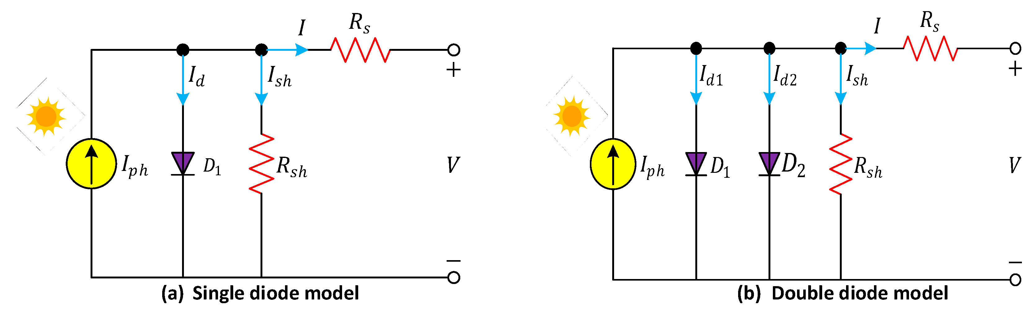
In the literature, single diode model (SDM) and double diode model (DDM) are widely used electrical models [9]. SDM is the simplest and most practical model of PV cell. This model has 5 unknown parameters, namely photogeneration current ( I p h ), shunt resistance ( R s h ), series resistance ( R s ), diode saturation current ( I d ) and ideality factor ( a ). The DDM, obtained by connecting a second diode in parallel, is the electrical model used for more complex and precise calculations with 7 unknown parameters [10]. In this context, the main objective of the calculation of unknown parameters is to design a PV cell model that will provide high accuracy and maximum power efficiency [7,10,11]. One of the main challenges is to solve the nonlinear equation provided by these designed models and to determine the unknown parameters. Several methods including analytical, deterministic and meta-heuristic (MH) have been proposed in the literature to improve the efficiency of PV systems [12]. Although analytical methods give fast results, they cause deviations in measured and calculated parameter values due to their dependence on initial values. Deterministic methods such as Newton-Raphson (NR), Gauss-Seidel have disadvantages such as high computation times [13,14]. Despite the disadvantages of analytical and deterministic approaches, MH optimisation methods have come to the fore [15].
In recent years, MH optimisation algorithms have been frequently used to solve many engineering problems. Optimisation algorithms in PV cells provide the most efficient and optimal results by analysing the interrelationships of the basic parameters of the cell in depth. This enables PV systems to be used more effectively by increasing energy efficiency [16,17,18]. There are some MH optimisation algorithms proposed in the literature such as atomic orbital search algorithm [19], bald eagle search (BES) [20], harris hawks optimization (HHO) [21], improved jaya optimization algorithm (IJAYA) [22], bacterial foraging algorithm (BFA) [23], tunicate swarm algorithm (TSA) [24], grey wolf optimization (GWO) [25], differential evolution (DE) [26], artificial bee swarm optimization (ABSO) [27], honey badger algorithm (HBA) [28], whale optimization algorithm (WOA) [29], farmland fertility optimizer (FFO) [30], ranking teaching learning based optimization (RTLBO) [31], wind driven optimization (WDO) [32], generalized oppositional teaching learning-based optimization (GOTLBO) [33], weighted mean of vectors algorithm (INFO) [34] etc. These algorithms provide solutions for parameter estimation in PV cells. However, current MH algorithms need to be investigated in more detail. In this context, it is important to introduce new optimisation algorithms for solar PV parameter extraction [35]. In this study, a novel frilled lizard optimisation (FLO) algorithm is proposed as an efficient method for estimating PV model parameters.
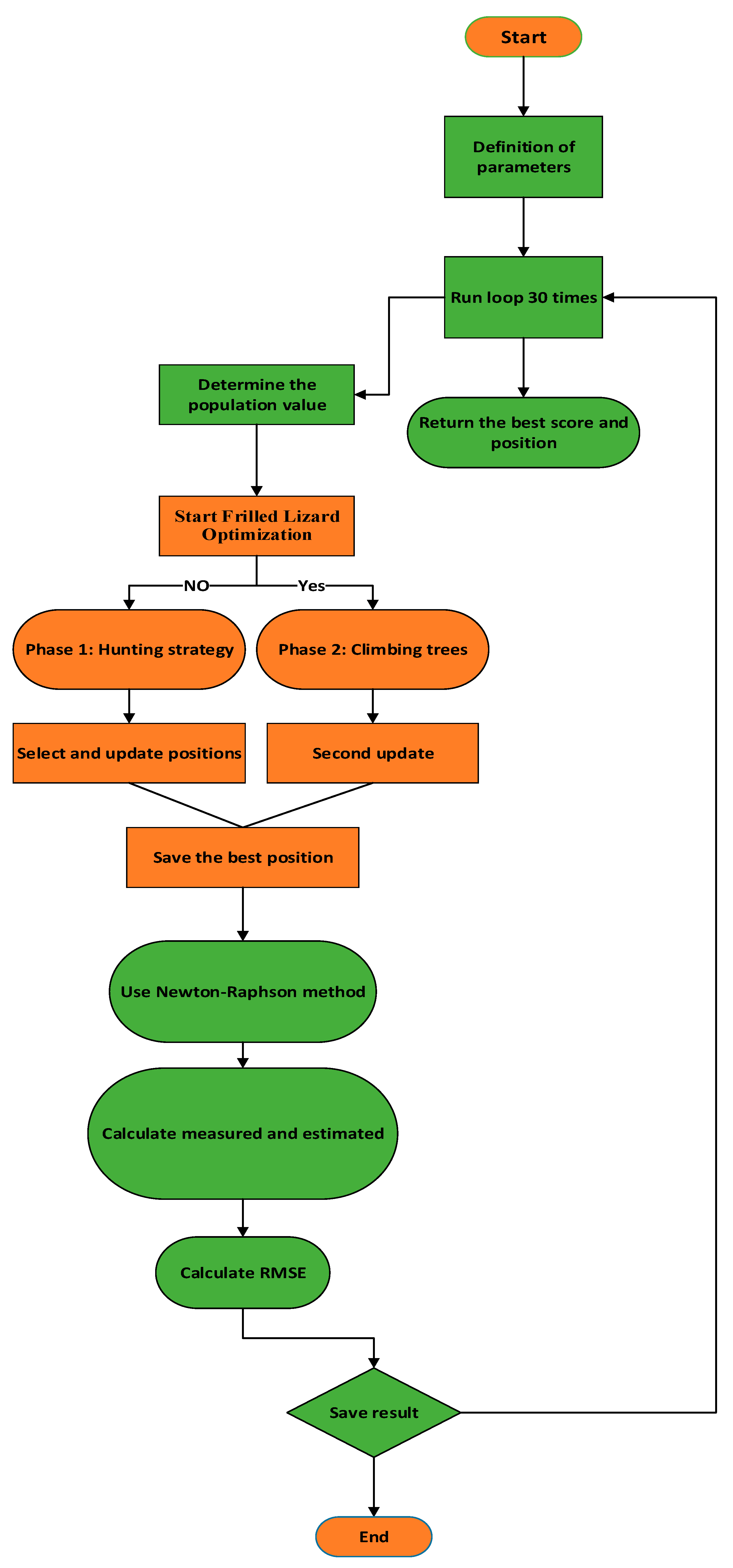
The FLO algorithm is inspired by the hunting and defence behaviour of the frilled lizard in nature and is devised to be used in solving complex problems. This optimisation algorithm is widely used in engineering, finance, energy management and health sciences [36,37,
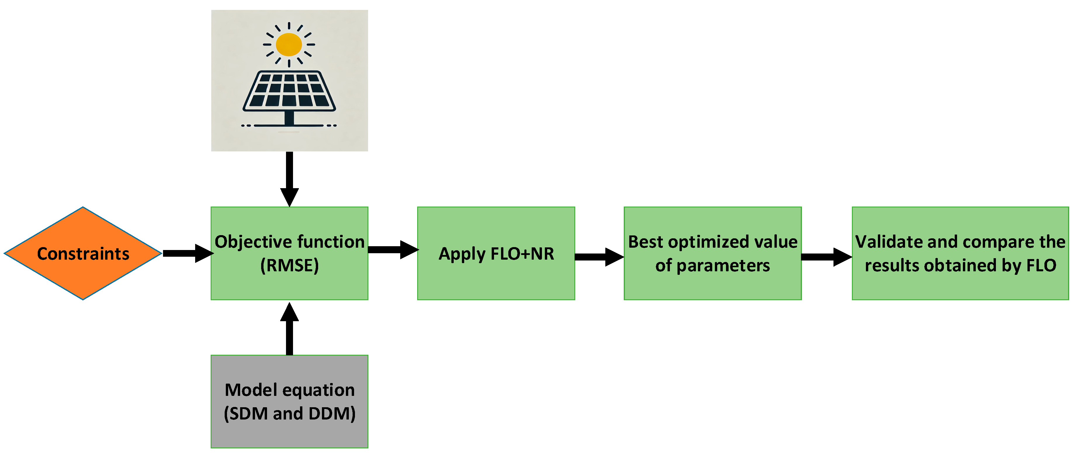
38]. The FLO algorithm has a population-based approach and works with an initially randomly generated solution set. The objective function, which evaluates how good the solution is to achieve the target value, is critical for optimisation algorithms [39,40,41]. In the optimisation of PV system parameters, the statistical term root mean square error (RMSE) is often used as the objective function. In this process, the decrease of the RMSE value in each iteration is an indication of improved performance. Since the relationship between current and voltage is nonlinear, the Newton-Raphson (N-R) numerical method is integrated to determine the solution points of the equations in the objective function [41,42,43]. In this paper, a novel FLO algorithm is integrated with the N-R numerical method and used for the first time in the literature to solve the problem of estimating unknown parameters in PV cells.
This paper contributes to the literature both theoretically and practically by developing a new methodology for the optimisation of PV cells. The first use of the FLO algorithm in this field fills an important gap in the literature and breaks new ground to inspire future studies. In this context, the study offers an innovative perspective both theoretically and practically. The main contributions of this study can be listed as follows:
  • A novel and efficient FLO algorithm is used to estimate the unknown parameters in PV systems.
  • In particular, the N-R numerical method is integrated to analyse the nonlinear equation of RMSE more efficiently.
  • The performance of the proposed FLO algorithm is also calculated in detail with error metrics such as IAE, RE, MAE.
  • A comprehensive comparison of the obtained results with various algorithms found in the literature has been made.
In the following Section 2, the mathematical formulation of the electrical models to be analysed and the objective function are introduced. Section 3 further details the proposed FLO algorithm. In Section 4, the experimental results obtained are evaluated and discussed. The last Section 5 is organised in such a way that a conclusion is presented.

2. Mathematical Model of Solar Cells

In the literature, although there are different PV solar cell models, SDM and DDM are widely used. [44]. In this study, two models given in Figure 2 will be used to analyse the current-voltage characteristics of PV cell models in depth. The mathematical expressions of these models and the objective function are analysed in detail in the following sections.
Figure 1. Equivalent circuit of photovoltaic models.
Preprints 142556 g001

2.1. Singe Diode Model

The SDM is a model often used to analyse PV cell characteristics [45]. As the electrical circuit is shown in Figure 1 (a), the general cycle formula of the model is expressed in equation (1) with Kirchhoff Current Law (KCL) [46].
I = I P h I d I s h
Also, R s , R s h , V , and I represent the series resistance, shunt resistance, output voltage and output current of the solar cell, respectively.
I d = I 0 e V + I * R s a * V t 1
V t = k * T q
In Equation (2), the diode current I d is expressed mathematically. I 0 and a are defined as diode saturation current and diode ideality factor, respectively. Equation (3), V t is the thermal voltage. k , T , and q are Boltzmann's constant (1.3806503 × 10²³ J/K), cell temperature in kelvin (K), and electron charge (1.60217646 × 10⁻¹⁹ C), respectively. The shunt resistor current I s h is mathematically defined in equation (4).
I s h = V + I * R s R s h
The output current of the SDM model can be rewritten as expressed in equation (5) [47].
I = I p h I 0 e V + I R s α V t 1 V + I R s R s h
Here, five unknown parameters ( I p h , I 0 , a , R s , R s h ) must be extracted to obtain the I-V characteristic of the SDM accurately.

2.2. Double Diode Model

As the electrical circuit is shown in Figure 1 (b), the DDM model is formed by connecting a second diode in parallel. The output current of the model is mathematically expressed by equation (6) by applying KCL [46].
I = I p h I d 1 I d 2 I s h
Where I d 1   is the first diode current and I d 2 is second diode current. Equations (7) and (8) describe these diode currents mathematically [46,47].
I d 1 = I 01 e V + I * R s a 1 * V t 1
I d 2 = I 01 e V + I * R s a 2 * V t 1
Here, we denote the saturation currents of the first and second diodes as I 01 and I 02   respectively, and the ideality factors as a 1 and a 2 respectively. V t was previously expressed in equation (3). Thus, the output current may be mathematically reformulated as presented in equation (9) [46,47].
I = I p h I 01 e V + I * R s a 1 * V t 1 I 02 e V + I * R s a 2 * V t 1 V + I R s R s h
Equation (9) expresses the output current of the DDM. Here, seven unknown parameters ( I p h , I 01 , I 02 , a 1 , a 2 , R s , R s h ) must be extracted for optimum operating conditions.

2.3. Objective Function

In the literature, there are various efficiency measures for parameter extraction in PV solar cells. The main purpose of the objective function is to minimise the difference between the estimated and measured parameter values. In this study, the root mean square error (RMSE) is used as the objective function. The error function of the model is expressed mathematically in equations (10) and (11) [46,48]. Furthermore, the model performance was rigorously evaluated using error metrics such as individual absolute error (IAE), relative error (RE) and mean absolute error (MAE), which are widely used in the literature. Through these error metrics, expressed mathematically in Equations (12), (13), (14), (15) and (16), the differences between the measured and estimated parameter values are examined in detail and the accuracy of the model is analysed comprehensively [1].
O b j e c t i v e   F u n c t i o n = 1 N i = 1 N J V ,   I ,   x 2
R M S E x = 1 N i = 1 N J I i m e a s u r e d I i e s t i m a t e d 2
I A E I = i = 1 N I m e a s u r e d I e s t i m a t i o n
I A E P = i = 1 N P m e a s u r e d P e s t i m a t i o n
R E I = I m e a s u r e d I e s t i m a t i o n I m e a s u r e d * 100
R E P = P m e a s u r e d P e s t i m a t i o n I m e a s u r e d * 100
M A E = 1 N i = 1 N I m e a s u r e d I e s t i m a t i o n

3. Frilled Lizard Optimization (FLO)

Frilled lizard optimisation (FLO) is an optimisation algorithm inspired by the behaviour of frilled lizards in hunting, moving towards prey and protecting against predators. This algorithm, which aims to solve complex problems, consists of 2 independent basic parts. These are exploration and exploitation phases [37,39].

3.1. Exploration Phase

This phase starts by imitating the ambush and movement of frilled lizards towards their prey. The main goal here is to find better solutions to solve the problem by looking at various regions. Then, using the hunting strategy of frilled lizards, the positions of individuals are updated by observing their positions and objective function values. In other words, individuals update their own positions by targeting other individuals that perform the best according to their own situation. By this design, the frilled lizard algorithm determines the potential prey points according to equation (17) [37,39].
C F L i = X i F k < F i ve k i
In this equation, C F L i represents the location of the prey of the i 'th individual. Here, it is aimed not to move away from the best value by taking into account the objective function values of other individuals. The position update in the next step is expressed by the following equation [37,39].
X i , j * = x i , j + r i , j S P i , j I i , j x i , j
In this equation, X i , j *   is the new updated position value, x i , j is the current position value, S P i , j is the target position value, r i , j is a random factor, I i , j is a factor determining the influence of other individuals. In equation (19), a mathematical representation of the conditions under which the new position value will be accepted is given [37,39].
X i = X i , j * , F i , j * < F i X i , otherwise
In the above equation, F i , j * and F i refer to the target function of the new position and the target function of the existing function respectively.

3.2. Exploitation Phase

This phase mimics the behaviour of a frilled lizard after being hunted, climbing a nearby tree to find a safe area. The main objective of this phase is to optimise the parameters found in the exploration phase. For this purpose, it is aimed to obtain more efficient solutions by analysing the previously found regions in depth. In this phase, each position update is represented by the following mathematical equation [37,39].
X i , j t + 1 = x i , j + 1 2 r U best L best
In the above equation X i , j ( t + 1 ) is the updated position in the second stage, x i , j is the current position, U best is the best solution found, L best is the worst solution found and r is a random factor. The following equation is then used to determine whether or not to accept the new found position [37,39].
X i = X i , j t + 1 , F i , j t + 1 < F i X i , otherwise
Figure 2 shows the overall process of the study, which systematically describes an optimised methodology for PV parameter estimation. The proposed FLO algorithm integrates the N-R mathematical approach, which is often preferred for solving nonlinear equations. Accurate calculation of I-V characteristics is an extremely significant criterion in solar cell modelling and parameter estimation. In this regard, the FLO+NR method combines strong global optimisation capabilities and fast convergence to determine the parameters with high accuracy. [41,42]. The flowchart of the FLO algorithm is presented in Figure 3.
Figure 2. An overview of FLO algorithm-based parameter estimation of PV models.
Preprints 142556 g002
Figure 3. FLO flowchart.
Preprints 142556 g003
Table 1. The upper and lower bounds of each parameter.
R.T.C France Module STM6-40/36 Module Photowatt-PWP201 Module
Parameters UpperBound LowerBound UpperBound LowerBound UpperBound LowerBound
I p h (A) 1 0 2 0 2 0
R s (Ω) 0,5 0 0,36 0 2 0
R s h (Ω) 100 0 1000 0 2000 0
a , a 1 2 1 60 1 50 1
I 0 , I 01 (µA) 1 0 50 0 50 0

4. Result And Discussion

In this section, the results obtained with the proposed FLO algorithm for the parameter estimation problem of solar PV cells are presented. In order to verify the effectiveness of the FLO algorithm, real current-voltage data from the literature were used. These data sets include R.T.C. France commercial silicon solar cell with a diameter of 57 mm, measured at 1000 W/m² irradiance and 33 °C, monocrystalline STM6-40/36 module measured at 51 °C and Photowatt-PWP201 module consisting of 36 cells connected in series measured at 45 °C [49,50]. All these analyses were performed using the electrical circuits of the SDM and DDM models, especially the lower and upper parameter limits of the data sets are given in Table 1. These bound values are critical values that determine the performance and efficiency characteristics of the modules [51]. The measured and predicted current-voltage (I-V), power-voltage (P-V) graphs, convergence curves and maximum power point (MPP) are given in detail with the proposed FLO algorithm. In addition, statistical metrics such as maximum (max), minimum (min), standard deviation (std), mean (mean), variance (var) and scatter plots are presented. In order to make a more powerful analysis, error metrics such as IAE, RE, MAE were calculated in addition to the RMSE used as the objective function, and the differences between the measured and estimated parameter values were analysed comprehensively. All these experiments were analysed using MATLAB R2022a software with Intel(R) Core(TM) i7-7500U CPU @ 2.70GHz 2.90 GHz and 8 GB RAM. In addition, the FLO algorithm proposed in the study was tested in 30 runs, 40 population sizes and 800 iterations.

4.1. Result for R.T.C. France

Table 2 shows that the FLO algorithm exhibits superior performance in optimisation accuracy for the SDM model. The lowest RMSE value of 0.0030375 was obtained when compared with multi-verse optimization (MVO), hybrid particle swarm optimization and simulated annealing (HPSOSA), bacterial foraging algorithm (BFA), genetic algorithm (GA), simulated annealing (SA), pattern search (PS), whale optimization algorithm (WOA), butterfly optimization algorithm (BOA) optimisation algorithms in the literature. Table 3 presents the optimisation results of the DDM model. The lowest RMSE value with 0.011538 was obtained compared to particle swarm optimization (PSO), opposition-based sine cosine algorithm (OBSCA), GA, SA, PS, WOA, BOA optimisation algorithms in the literature. These results demonstrate the superior performance of the proposed method in parameter estimation on SDM and DDM models.
Table 2. Comparison of result obtained from the FLO with other optimization techniques in the literature for SDM.
Algorithm I p h (A) I o (μA) R s (Ω) R s h (Ω) α RMSE
FLO (Proposed) 0.761598 0.384977 0.0381659 68.8525 1.49892 0.0030375
MVO [44] 0.7616 0.32094 0.0365 59.5884 1.5252 0.1268
HPSOS [44] 0.7608 0.3117 0.0365 52.8898 1.4753 0.0071
BFA [52] 0.7602 0.8000 0.0325 50.8691 1.6951 0.029
GA[52] 0.7619 0.8087 0.0299 43.3729 1.5751 0.019
SA [53] 0.762 0.4798 0.0345 43.1034 1.5172 0.019
PS [54] 0.7617 0.998 0.0313 64.1026 1.6 0.2863
WOA [55] 0.76405 0.28588 0.0484 59.9940 1.4702 0.0132
BOA [56] 0.760234 0.80980 0.023287 30.53997 1.585917 0.16641
Figure 4 (a) and (b) show the I-V and P-V characteristic curves of the SDM model, respectively. When these curves are analysed, it is clearly seen that the measured and predicted values agree with a high accuracy. Likewise, Figure 5 (a) and (b) show this agreement in the I-V and P-V characteristic curves of the DDM model, respectively. In this regard, these graphs strongly support the accuracy and reliability of both the model and the FLO algorithm used. In Figure 6 (a) and (b), the convergence curves of SDM and DDM are presented respectively. The fact that the fitness values for both models reach low levels proves that the solution accuracy of the algorithm is high. It is also evident that the FLO algorithm performs reliably and efficiently for both simple and complex models.
Table 4 presents the measured and estimated current and power values of the SDM model and the error metrics such as IAE, RE, MAE between these values in a comprehensive manner. In this regard, it is clearly seen that I m and P m values agree with I e and P e values with a high level of accuracy. Analysing the determined error metrics, the total IAE error value in the SDM model was calculated as 0.06194 and 0.02812 for current and power, respectively. The MAE error value was calculated depending on the IAE values for each data line in order to analyse the change in the process, and the total MAE error value was obtained as 0.00238 for current.
Table 5 shows the error metrics of the DDM model. Here, the total IAE error value is calculated as 0.27738 and 0.10030 for current and power, respectively. The MAE error value was calculated depending on the IAE values for each data line in order to analyse the change in the process, and the total MAE error value was obtained as 0.01067 for current. The low error values for SDM and DDM model are important indicators of the consistency of the algorithm. Figure 7 (a) and (b) show that the agreement between measured and estimated I-V/P-V values at all data points for the SDM and DDM models is clearly observed. In Figure 7 (c), a graphical representation of the IAE and MAE error performance for both models is presented. In addition, although the RE error metric results calculated for the current and power shown in Table 4 and Table 5 are quite consistent, deviations are experienced at certain data points. This situation can be interpreted as a need for improvements in the optimisation process of the proposed FLO algorithm. Considering all the analyses, SDM offers a simpler and faster modelling approach, while DDM stands out as an option that can be used in more complex situations. In terms of overall performance, it is evident that the FLO algorithm provides precise solutions to the parameter optimisation problem in PV cells by providing highly effective results in both models.

4.2. Results For STM6-40/36 and Photowatt-PWP201

In this subsection, the optimal parameters obtained with the FLO algorithm using the STM6-40/36 data set are presented in Table 6. The lowest RMSE value of 0.012036 was obtained when compared with triple archives particle swarm optimization (TAPSO), artificial bee colony (ABC), chaotic improved artificial bee colony (CIABC), PSO, sine–cosine algorithm (SCA), wind driven optimization (WDO) optimisation algorithms in the literature. In particular, this shows that the estimated parameter values are highly accurate. The I-V and P-V characteristic curves in Figure 8 (a) and (b) show that the agreement between the measured and estimated values is very strong. In Table 7, the lowest RMSE value with 0.012036 was obtained in the analysis using Photowatt-PWP201 module compared to whale optimization algorithm (WOA), SCA, firefly algorithm (FA), atom search optimization (ASO), newton, WDO. As shown in Figure 9 (a) and (b), the measured and estimated values are quite consistent. The convergence curves of STM6-40/36 and Photowatt-PWP201 are presented in Figure 10 (a) and (b), respectively. In both models, the FLO algorithm showed a fast convergence with early iteration. This proves that the algorithm has a strong exploration capability and can effectively scan the solution space. As a result, it shows that the FLO algorithm exhibits a strong performance in both convergence speed and solution accuracy and works effectively in parameter estimation tasks for different PV modules.
In Table 8 and Table 9, measured and predicted current and power values of STM6-40/36 and Photowatt-PWP201 models, respectively, as well as calculated error metrics are given. As shown in Table 8, the calculated total IAE is 0.1529 and 2.4106 for current and power error values, respectively. The MAE error value was calculated depending on the IAE values for each data line in order to analyse the change in the process, and the total MAE error value was obtained as 0.0076 for current. In Table 9, the total IAE error values for current and power are calculated as 0.1856 and 2.6810, respectively, and the total MAE error value for current is calculated as 0.0074. Figure 11 (a) and (b) shows the consistency between measured and predicted I-V/P-V values at all data points for STM6-40/36 and Photowatt-PWP201 modules. In Figure 11 (c) and (d), a graphical approach including the IAE and MAE error performance for both models is presented. Furthermore, Table 8 and Table 9 show the error metric results of these models for current and power. The low error values obtained clearly demonstrate that the proposed FLO algorithm produces highly consistent and reliable solutions for different PV module data sets.
Table 10 statistically evaluates the modelling performance using the RMSE values calculated by the FLO algorithm with SDM, DDM, STM6-40/36 and Photowatt-PWP201 module data. Max, Min, Mean, Std and Var values are presented for each data set. Also, a graph showing the error distribution of these metrics is given in Figure 12. In STM6-40/36, the max. error value (1.54332) is higher than the other data sets. In Photowatt-PWP201, the max. RMSE value (0.43731) is higher than SDM and DDM models. In this respect, high max. values can be interpreted as the algorithm should be improved on these data sets. The minimum RMSE values are 0.01153 and 0.01203 for DDM and STM6-40/36, respectively, and although these values are higher compared to SDM and Photowatt-PWP201 (0.00303 and 0.00975, respectively), the RMSE values in all analysed module data remain at a low level in general.This indicates that the model has a high accuracy capacity. Mean RMSE is the lowest in the SDM (0.08168) and DDM (0.08529) models. This indicates that the errors for the two models are in a narrow range. The error values are slightly higher for the STM6-40/36 (0.69211) and Photowatt-PWP201 (0.21988) models. In this respect, it may indicate that the proposed optimisation method should be improved in order to increase the performance of the models. Std. and var. values (0.33856 and 0.11462, respectively) are the highest for the STM6-40/36 module. This indicates that the errors are distributed in a wider range for this data set. All these results show that the proposed FLO algorithm performs well in terms of overall accuracy and consistency, but the optimisation process can be improved for some data sets (STM6-40/36 and Photowatt-PWP201).
In Table 11, the FLO algorithm obtained high accuracy results compared to hybrid firefly algorithm and pattern search algorithm (HFAPS) bird mating optimization (BMO), firefly algorithm (FA) comparing the maximum power point (MPP) parameters ( V M P , I M P , P M P ) to evaluate its performance. For the R.T.C France dataset, V M P , I M P , P M P values (respectively: 0.459, 0.67352, 0.30915) were estimated with very small deviation compared to the measured values. Similarly, the values obtained for STM6-40/36 dataset (respectively: 16.98, 1.504, 25.5381) produced more accurate results than the other algorithms compared. In the Photowatt PWP-201 dataset, the values estimated by the proposed FLO algorithm (respectively: 12.4929, 0.9256, 11.5634) proved its potential with the closest deviation to the measured values compared to other algorithms. Since BMO, FA and HFAPS algorithms exhibit higher deviations, the proposed FLO algorithm stands out as a promising alternative in terms of its overall performance in estimating MPP parameters accurately and reliably.

4.4. Discussion

The performance of the FLO algorithm is evaluated, and various analyses are performed in this study. In these analyses; 3 reference PV models, namely R.T.C France, STM6-40/36, Photowatt-PWP201 data sets, were used. The FLO algorithm stands out with its low RMSE values obtained for both SDM and DDM models tested with R.T.C France module data. In the SDM model, FLO outperformed the other compared algorithms with a very low RMSE value of 0.0030375. It is especially more successful compared to methods such as HPSOS (0.0071) and BFA (0.029). In the DDM model, FLO's RMSE value of 0.011538 is lower than popular optimisation methods such as SA (0.01664) and PSO (0.0166). These results show that the proposed algorithm is effective for parameter optimisation in PV systems. In addition, in the comparative analysis with the SDM model with STM6-40/36 module data, more successful results were obtained than the compared algorithms (such as TAPSO: 0.013423, CIABC: 0.02518) with an RMSE value of 0.012036. In the analysis performed with Photowatt-PWP201 module data, FLO has been strongly proven to achieve much more successful results compared to algorithms such as WOA (0.2838) and SCA (0.0117780) by providing the lowest error rate with an RMSE value of 0.0097545. It is evident that the proposed FLO algorithm provides more consistent and accurate parameter extraction than MVO, HPSOSA, BFA, GA, SA, PS, WOA, BOA, PSO, OBSCA, TAPSO, ABC, SCA, CIABC, WDO, FA, ASO, newton optimisation techniques. Although these methods are successful in specific parameter extraction, the overall performance of FLO is stronger in terms of accurate estimation of all parameters. Moreover, in order to test the accuracy of the measured and estimated parameter values, error metrics such as IAE, RE, MAE are also calculated and given in Tables 4, 5, 8 and 9. Furthermore, for each analysed model, the measured and estimated parameter values are compared in Figures 4, 5, 8 and 9 and the convergence curves of the proposed FLO algorithm are presented in Figure 6 and Figure 10. All these analysis results show that the proposed algorithm provides accurate solutions in both theoretical and practical applications.

5. Conclusions

In this paper, a novel FLO algorithm is proposed to estimate the unknown parameters in PV cells and N-R numerical method is integrated to improve the efficiency of the algorithm. In order to reveal the potential of the algorithm, analyses were performed on single and dual diode electrical models using R.T.C Fance, STM6-40/36 and Photowatt-PWP-201 real module data. In addition, IAE, RE and MAE error metrics were calculated. These error metric results, the lowest RMSE value obtained compared to other compared algorithms, consistent statistical metrics (such as max, min, mean, std, var) and highly accurate matched MPP point, suggest that the proposed FLO algorithm offers a powerful alternative that increases efficiency with precise parameter estimation, especially in PV cells. Furthermore, it is shown that the proposed FLO algorithm provides a strong agreement and parallelism between the I-V and P-V characteristics of the measured and estimated parameter values. As a result, FLO has a wide application potential in the design and performance analyses of solar energy systems. Especially, it is an effective tool for efficiency analyses of photovoltaic modules, simulation of panel performance and improving accuracy in system design. In addition, FLO's low error rates and results compatible with physical parameters support its use in the industrial field. This algorithm is expected to be useful in industrial applications to provide optimum design and efficiency in solar energy systems. The following topics are planned to be focussed in future studies.
  • The FLO algorithm will make significant contributions to the development of PV cell models in a more dynamic way through hybrid approaches created by integration with different algorithms.
  • Experimental studies will be carried out with module data including different operating conditions in order to verify the practical effectiveness of the FLO algorithm.
  • Studies will be carried out on the applicability of FLO algorithm to the solution of optimisation problems in various fields.
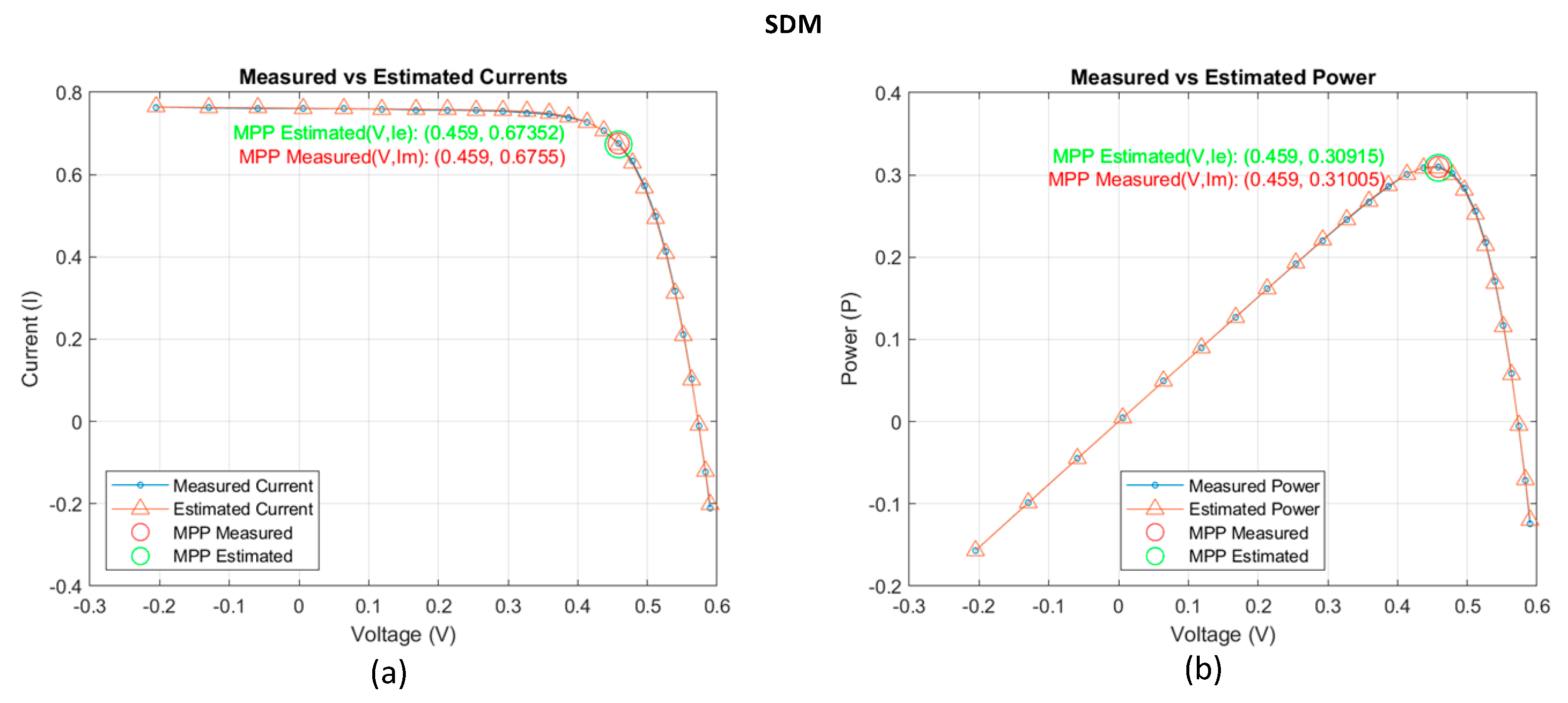
References

  1. Sharma, P. and S. Raju, Efficient estimation of PV parameters for existing datasets by using an intelligent algorithm. Optik, 2023. 295: p. 171467. [CrossRef]
  2. Nyamathulla, S., D. Chittathuru, and S. Muyeen, An overview of multilevel inverters lifetime assessment for grid-connected solar photovoltaic applications. Electronics, 2023. 12(8): p. 1944. [CrossRef]
  3. Kumar, D., et al., A novel hybrid MPPT approach for solar PV systems using particle-swarm-optimization-trained machine learning and flying squirrel search optimization. Sustainability, 2023. 15(6): p. 5575. [CrossRef]
  4. Dadkhah, J. and M. Niroomand, Optimization methods of MPPT parameters for PV systems: review, classification, and comparison. Journal of Modern Power Systems and Clean Energy, 2021. 9(2): p. 225-236. [CrossRef]
  5. Hazim, H.I., et al., Review on optimization techniques of PV/inverter ratio for grid-Tie PV systems. Applied Sciences, 2023. 13(5): p. 3155. [CrossRef]
  6. Águila-León, J., et al., Optimizing photovoltaic systems: a meta-optimization approach with GWO-Enhanced PSO algorithm for improving MPPT controllers. Renewable Energy, 2024. 230: p. 120892.
  7. Elhammoudy, A., et al., Dandelion Optimizer algorithm-based method for accurate photovoltaic model parameter identification. Energy Conversion and Management: X, 2023. 19: p. 100405. [CrossRef]
  8. Raheem, F.S. and N. Basil, Automation intelligence photovoltaic system for power and voltage issues based on Black Hole Optimization algorithm with FOPID. Measurement: Sensors, 2023. 25: p. 100640. [CrossRef]
  9. Yang, B., et al., Comprehensive overview of meta-heuristic algorithm applications on PV cell parameter identification. Energy Conversion and Management, 2020. 208: p. 112595. [CrossRef]
  10. Venkateswari, R. and N. Rajasekar, Review on parameter estimation techniques of solar photovoltaic systems. International Transactions on Electrical Energy Systems, 2021. 31(11): p. e13113. [CrossRef]
  11. Garip, Z., Parameters estimation of three-diode photovoltaic model using fractional-order Harris Hawks optimization algorithm. Optik, 2023. 272: p. 170391. [CrossRef]
  12. Khan, F., A. Al-Ahmed, and F.A. Al-Sulaiman, Critical analysis of the limitations and validity of the assumptions with the analytical methods commonly used to determine the photovoltaic cell parameters. Renewable and Sustainable Energy Reviews, 2021. 140: p. 110753. [CrossRef]
  13. Zhang, H., et al., Orthogonal Nelder-Mead moth flame method for parameters identification of photovoltaic modules. Energy Conversion and Management, 2020. 211: p. 112764. [CrossRef]
  14. Lu, Y., et al., Hybrid multi-group stochastic cooperative particle swarm optimization algorithm and its application to the photovoltaic parameter identification problem. Energy Reports, 2023. 9: p. 4654-4681. [CrossRef]
  15. Navarro, M.A., et al., An analysis on the performance of metaheuristic algorithms for the estimation of parameters in solar cell models. Energy Conversion and Management, 2023. 276: p. 116523. [CrossRef]
  16. El-Dabah, M.A., et al., Photovoltaic model parameters identification using Northern Goshawk Optimization algorithm. Energy, 2023. 262: p. 125522. [CrossRef]
  17. Duan, Z., et al., Parameter extraction of solar photovoltaic model based on nutcracker optimization algorithm. Applied Sciences, 2023. 13(11): p. 6710. [CrossRef]
  18. Abd El-Mageed, A.A., et al., Parameter extraction of solar photovoltaic models using queuing search optimization and differential evolution. Applied Soft Computing, 2023. 134: p. 110032. [CrossRef]
  19. Ali, F., et al., Parameter extraction of photovoltaic models using atomic orbital search algorithm on a decent basis for novel accurate RMSE calculation. Energy Conversion and Management, 2023. 277: p. 116613. [CrossRef]
  20. Nicaire, N.F., et al., Parameter estimation of the photovoltaic system using bald eagle search (BES) algorithm. International Journal of Photoenergy, 2021. 2021(1): p. 4343203. [CrossRef]
  21. Qais, M.H., H.M. Hasanien, and S. Alghuwainem, Parameters extraction of three-diode photovoltaic model using computation and Harris Hawks optimization. Energy, 2020. 195: p. 117040. [CrossRef]
  22. Rao, R., Jaya: A simple and new optimization algorithm for solving constrained and unconstrained optimization problems. International Journal of Industrial Engineering Computations, 2016. 7(1): p. 19-34. [CrossRef]
  23. Rajasekar, N., N.K. Kumar, and R. Venugopalan, Bacterial foraging algorithm based solar PV parameter estimation. Solar Energy, 2013. 97: p. 255-265. [CrossRef]
  24. Sharma, A., et al., Parameter extraction of photovoltaic module using tunicate swarm algorithm. Electronics, 2021. 10(8): p. 878.
  25. Nayak, B., A. Mohapatra, and K.B. Mohanty, Parameter estimation of single diode PV module based on GWO algorithm. Renewable Energy Focus, 2019. 30: p. 1-12. [CrossRef]
  26. Pant, M., et al., Differential Evolution: A review of more than two decades of research. Engineering Applications of Artificial Intelligence, 2020. 90: p. 103479. [CrossRef]
  27. Askarzadeh, A. and A. Rezazadeh, Artificial bee swarm optimization algorithm for parameters identification of solar cell models. Applied energy, 2013. 102: p. 943-949. [CrossRef]
  28. Diab, A.A.Z., et al., Photovoltaic parameter estimation using honey badger algorithm and African vulture optimization algorithm. Energy Reports, 2022. 8: p. 384-393. [CrossRef]
  29. Xiong, G., et al., Parameter extraction of solar photovoltaic models using an improved whale optimization algorithm. Energy conversion and management, 2018. 174: p. 388-405. [CrossRef]
  30. Agwa, A.M., A.A. El-Fergany, and H.A. Maksoud, Electrical characterization of photovoltaic modules using farmland fertility optimizer. Energy Conversion and Management, 2020. 217: p. 112990. [CrossRef]
  31. Xiong, G., et al., Parameter identification of solid oxide fuel cells with ranking teaching-learning based algorithm. Energy Conversion and Management, 2018. 174: p. 126-137. [CrossRef]
  32. Derick, M., et al., An improved optimization technique for estimation of solar photovoltaic parameters. Solar Energy, 2017. 157: p. 116-124. [CrossRef]
  33. Chen, X., et al., Parameters identification of solar cell models using generalized oppositional teaching learning based optimization. Energy, 2016. 99: p. 170-180. [CrossRef]
  34. Izci, D., et al. Parameter estimation of solar cells via weighted mean of vectors algorithm. in 2022 Global Energy Conference (GEC). 2022. IEEE.
  35. Abbassi, R., et al., Identification of unknown parameters of solar cell models: A comprehensive overview of available approaches. Renewable and Sustainable Energy Reviews, 2018. 90: p. 453-474. [CrossRef]
  36. Fakhouri, H.N., et al., Hybrid Four Vector Intelligent Metaheuristic with Differential Evolution for Structural Single-Objective Engineering Optimization. Algorithms, 2024. 17(9): p. 417. [CrossRef]
  37. Abualigah, L., et al., Frilled Lizard Optimization to optimize parameters Proportional Integral Derivative of DC Motor. Vokasi Unesa Bulletin of Engineering, Technology and Applied Science, 2024: p. 14-21. [CrossRef]
  38. Nanibabu, S., S. Baskaran, and P. Marimuthu. Optimal Charging Scheduling of Electric vehicles for Smart Grid Operations Employing Demand Side Management strategy with Battery Storage System. in 2024 6th International Conference on Energy, Power and Environment (ICEPE). 2024. IEEE.
  39. Falahah, I.A., et al., Frilled Lizard Optimization: A Novel Bio-Inspired Optimizer for Solving Engineering Applications. Computers, Materials & Continua, 2024. 79(3).
  40. Hamadneh, T., et al., Magnificent Frigatebird Optimization: A New Bio-Inspired Metaheuristic Approach for Solving Optimization Problems. Computers, Materials and Continua, 2024. 80(2): p. 2721-2741. [CrossRef]
  41. Ayyarao, T.S., Parameter estimation of solar PV models with quantum-based avian navigation optimizer and Newton–Raphson method. Journal of Computational Electronics, 2022. 21(6): p. 1338-1356. [CrossRef]
  42. Gnetchejo, P.J., et al., A combination of Newton-Raphson method and heuristics algorithms for parameter estimation in photovoltaic modules. Heliyon, 2021. 7(4). [CrossRef]
  43. El-Sayed, M.I., M.A.-E.-H. Mohamed, and M.H. Osman. A novel parameter estimation of a PV model. in 2016 IEEE 43rd Photovoltaic Specialists Conference (PVSC). 2016. IEEE.
  44. Wang, M., et al., Evaluation of constraint in photovoltaic models by exploiting an enhanced ant lion optimizer. Solar Energy, 2020. 211: p. 503-521. [CrossRef]
  45. Stornelli, V., et al., A new simplified five-parameter estimation method for single-diode model of photovoltaic panels. Energies, 2019. 12(22): p. 4271. [CrossRef]
  46. Duman, S., et al., A powerful meta-heuristic search algorithm for solving global optimization and real-world solar photovoltaic parameter estimation problems. Engineering Applications of Artificial Intelligence, 2022. 111: p. 104763. [CrossRef]
  47. Premkumar, M., et al., Enhanced chaotic JAYA algorithm for parameter estimation of photovoltaic cell/modules. ISA transactions, 2021. 116: p. 139-166. [CrossRef]
  48. Messaoud, R.B., Extraction of uncertain parameters of single-diode model of a photovoltaic panel using simulated annealing optimization. Energy Reports, 2020. 6: p. 350-357.
  49. Easwarakhanthan, T., et al., Nonlinear minimization algorithm for determining the solar cell parameters with microcomputers. International journal of solar energy, 1986. 4(1): p. 1-12. [CrossRef]
  50. Tong, N.T. and W. Pora, A parameter extraction technique exploiting intrinsic properties of solar cells. Applied energy, 2016. 176: p. 104-115. [CrossRef]
  51. Yu, X., Y. Duan, and Z. Cai, Sub-population improved grey wolf optimizer with Gaussian mutation and Lévy flight for parameters identification of photovoltaic models. Expert Systems with Applications, 2023. 232: p. 120827. [CrossRef]
  52. Oliva, D., E. Cuevas, and G. Pajares, Parameter identification of solar cells using artificial bee colony optimization. Energy, 2014. 72: p. 93-102. [CrossRef]
  53. El-Naggar, K.M., et al., Simulated annealing algorithm for photovoltaic parameters identification. Solar Energy, 2012. 86(1): p. 266-274. [CrossRef]
  54. AlHajri, M., et al., Optimal extraction of solar cell parameters using pattern search. Renewable energy, 2012. 44: p. 238-245. [CrossRef]
  55. Oliva, D., M. Abd El Aziz, and A.E. Hassanien, Parameter estimation of photovoltaic cells using an improved chaotic whale optimization algorithm. Applied energy, 2017. 200: p. 141-154. [CrossRef]
  56. Long, W., et al., Parameters identification of photovoltaic models by using an enhanced adaptive butterfly optimization algorithm. Energy, 2021. 229: p. 120750. [CrossRef]
  57. Ye, M., X. Wang, and Y. Xu, Parameter extraction of solar cells using particle swarm optimization. Journal of Applied Physics, 2009. 105(9). [CrossRef]
  58. Yang, X. and W. Gong, Opposition-based JAYA with population reduction for parameter estimation of photovoltaic solar cells and modules. Applied Soft Computing, 2021. 104: p. 107218. [CrossRef]
  59. Beigi, A.M. and A. Maroosi, Parameter identification for solar cells and module using a hybrid firefly and pattern search algorithms. Solar Energy, 2018. 171: p. 435-446. [CrossRef]
  60. Issa, M., A.M. Helmi, and M. Ghetas, Estimation of solar cell parameters through utilization of adaptive sine–cosine particle swarm optimization algorithm. Neural Computing and Applications, 2024. 36(15): p. 8757-8773. [CrossRef]
  61. Mathew, D., et al., Wind-driven optimization technique for estimation of solar photovoltaic parameters. IEEE Journal of Photovoltaics, 2017. 8(1): p. 248-256. [CrossRef]
  62. Abdel-Basset, M., et al., An improved artificial jellyfish search optimizer for parameter identification of photovoltaic models. Energies, 2021. 14(7): p. 1867. [CrossRef]
  63. Yaghoubi, M., et al., Modified salp swarm optimization for parameter estimation of solar PV models. Ieee Access, 2022. 10: p. 110181-110194. [CrossRef]
  64. Tefek, M.F., Artificial bee colony algorithm based on a new local search approach for parameter estimation of photovoltaic systems. Journal of Computational Electronics, 2021. 20(6): p. 2530-2562. [CrossRef]
Figure 4. Comparison between the measured and the estimated data obtained by FLO algorithm for R.T.C France model (a) I-V of SDM, (b) P-V of SDM.
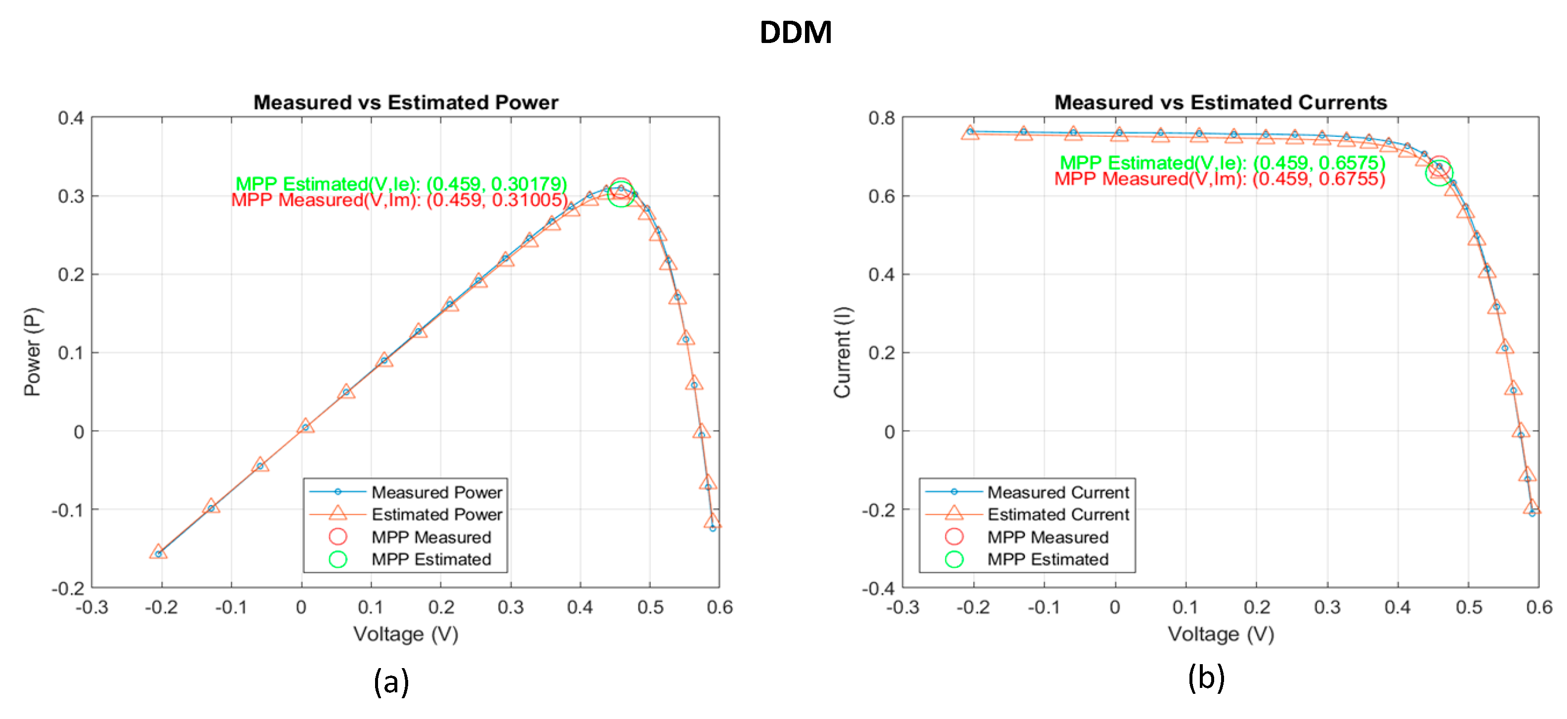
Preprints 142556 g004
Figure 5. Comparison between the measured and the estimated data obtained by FLO algorithm for R.T.C France model (a) I-V of DDM, (b) P-V of DDM.
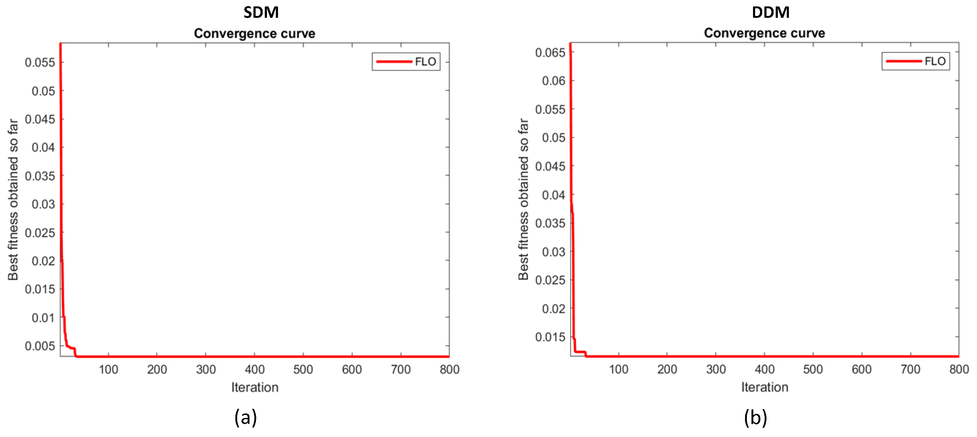
Preprints 142556 g005
Figure 6. Convergence graph of proposed FLO algorithm for R.T.C France model: (a) SDM, (b) DDM.
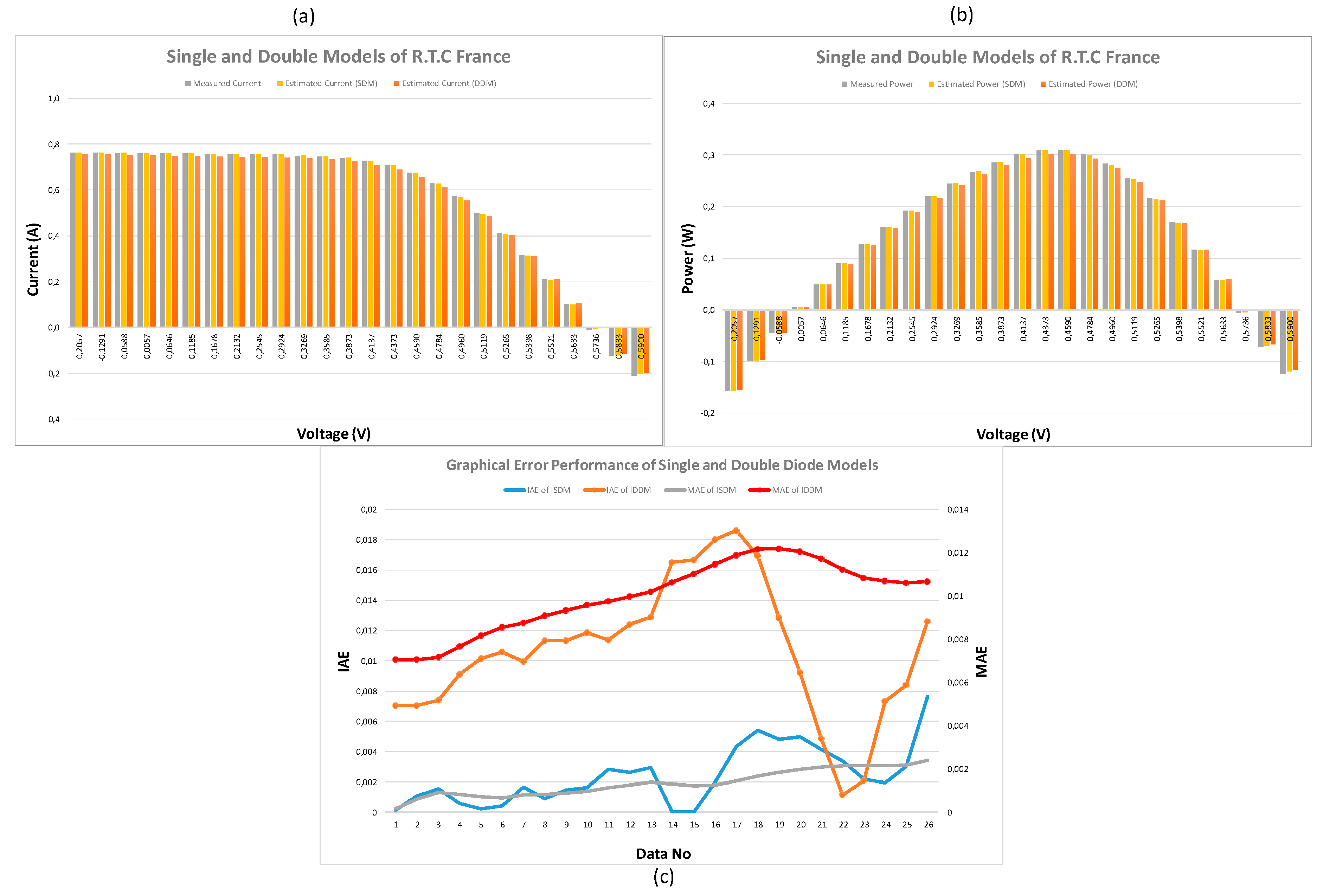
Preprints 142556 g006
Figure 7. Performance Comparison of Single and Double Diode Models Using FLO algorithm (a)I-V, (b)P-V and (c) Error Metrics for Each Data Point.
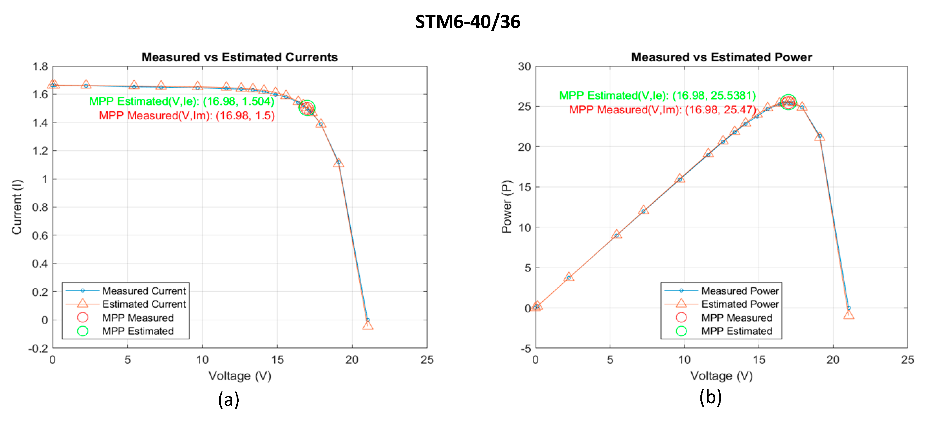
Preprints 142556 g007
Figure 8. Comparison between the measured and the estimated data obtained by FLO algorithm for STM6-40/36 model (a) I-V curve. (b) P-V curve.
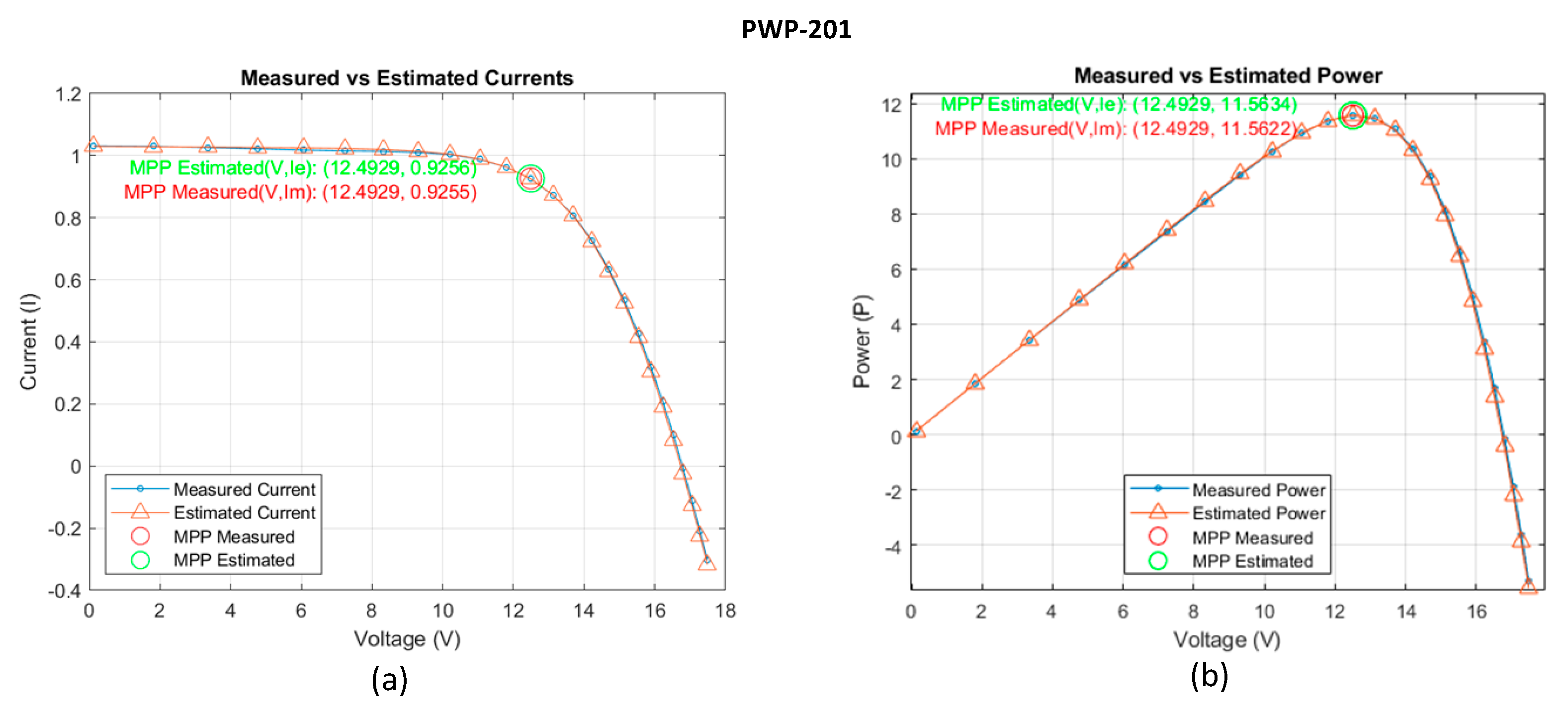
Preprints 142556 g008
Figure 9. Comparison between the measured and the estimated data obtained by FLO algorithm for Photowatt PWP-201 model (a) I-V curve. (b) P-V curve.
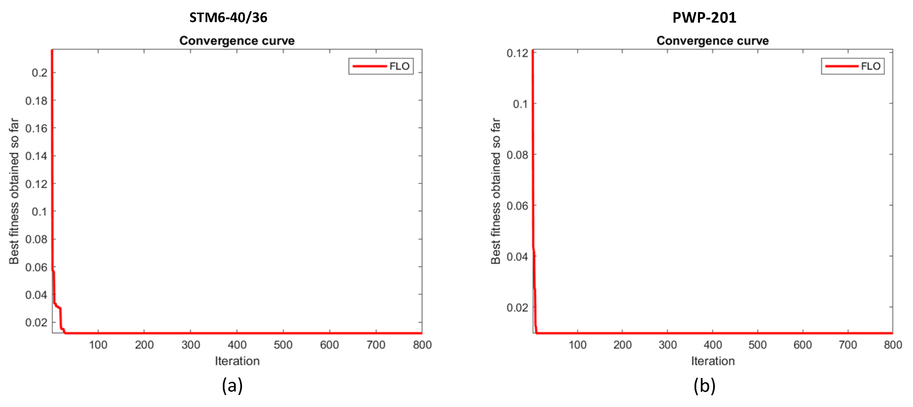
Preprints 142556 g009
Figure 10. Convergence graph of proposed FLO algorithm for: (a) STM6-40/36. (b) Photowatt PWP-201.
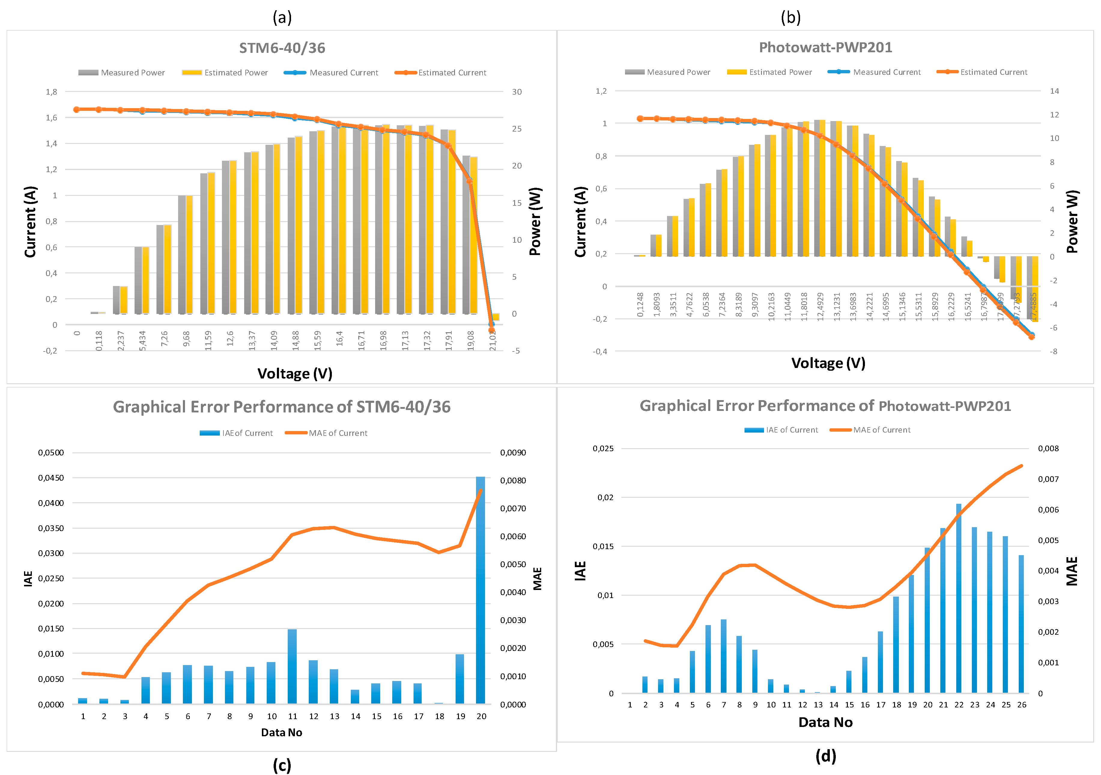
Preprints 142556 g010
Figure 11. Performance Comparison I-V, P-V and Error Metrics for Each Data Point; (a), (c) STM6-40/36 and (b), (d) Photowatt-PWP201.
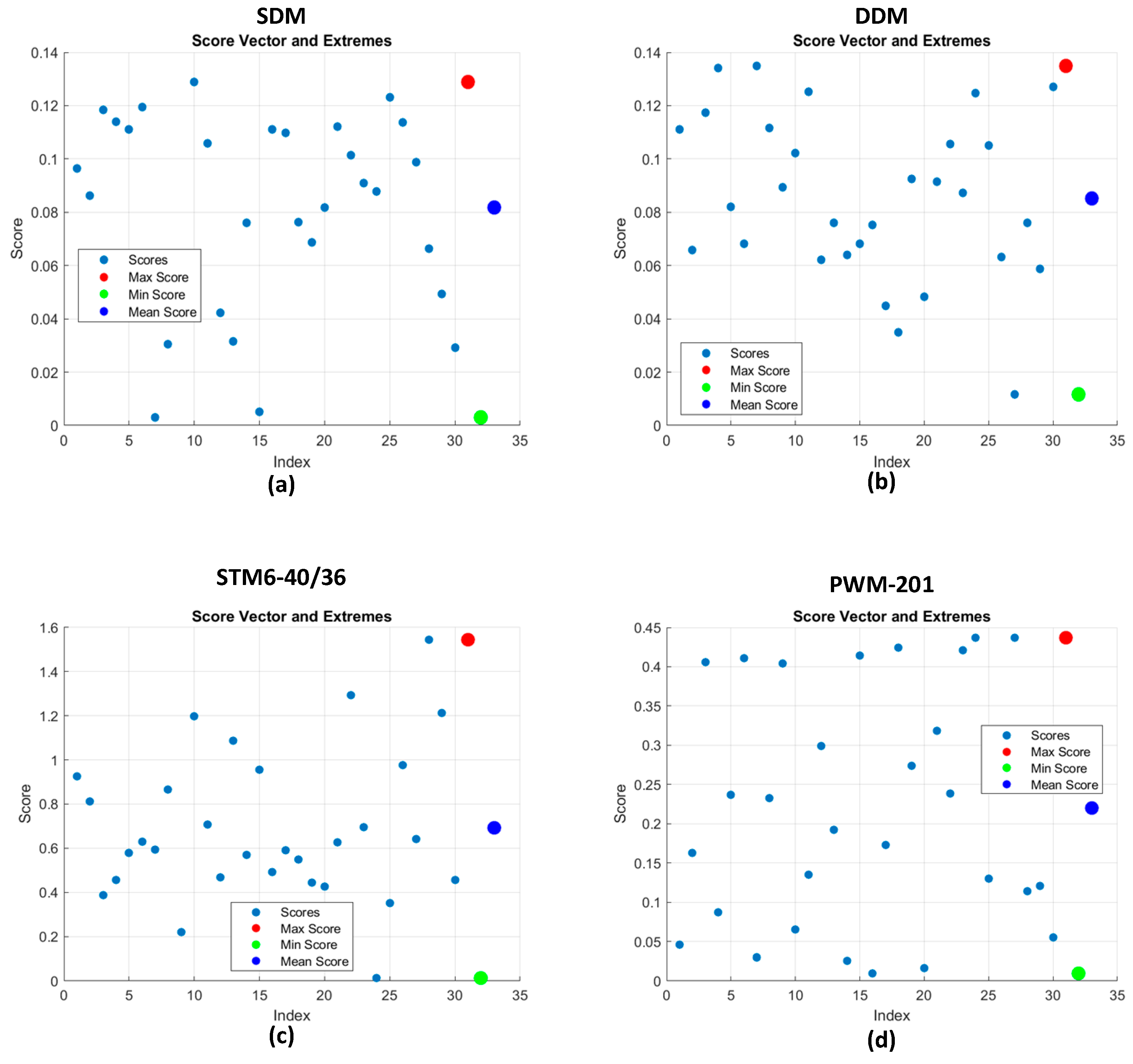
Preprints 142556 g011
Figure 12. Statistical scores (RMSE) of all runs (30) by FLO algorithm: (a) SDM. (b) DDM. (c) STM6-40/36 and (d) Photowatt PWP-201.
Preprints 142556 g012
Table 3. Comparison of result obtained from the FLO with other optimization techniques in the literature for DDM.
Algorithm I p h (A) I o 1 (μA) R s (Ω) R s h (Ω) α 1 I o 2 (μA) α 2 RMSE
FLO (Proposed) 0.752239 0.592485 0.0342579 38.0587 1.55789 0.646782 1.9019 0.011538
PSO [57] 0.7623 0.4767 0.0325 43.1034 1.5172 0.01 2 0.0166
GA [52] 0.7608 0.0001 0.0364 53.7185 1.3355 0.0001 1.481 0.36040
SA [53] 0.7623 0.4767 0.0345 43.1034 1.5172 0.01 2 0.01664
PS [54] 0.7602 0.9889 0.032 81.3008 1.6 0.0001 1.192 0.01518
WOA [55] 0.7658 2.9957E-07 0.0493 59.0196 1.4795 3.9438E-07 1.9201 0.0154
OBSCA [56] 0.794380 0.528673 0.03468 23.9696 1.527530 0.04440 2 0.024067
BOA [56] 0.78077 0.89987 0.03875 34.5559 1.47604 0.29385 1.99100 0.013564
Table 4. Statistical error tests for SDM of R.T.C. France.
No Measured Data Estimation Data IAE RE MAE
V V I m   A P m W I e   A P e W I A E I I A E P R E I R E P M A E I
1 -0.2057 0.7640 -0.1572 0.7642 -0.1572 0.00016 0.00004 0.0209 -0.0255 0.00016
2 -0.1291 0.7620 -0.0984 0.7631 -0.0985 0.00105 0.00014 0.1378 -0.1382 0.00060
3 -0.0588 0.7605 -0.0447 0.7620 -0.0448 0.00153 0.00009 0.2012 -0.2013 0.00091
4 0.0057 0.7605 0.0043 0.7611 0.0043 0.00059 0.00000 0.0776 0.0784 0.00083
5 0.0646 0.7600 0.0491 0.7602 0.0491 0.00023 0.00002 0.0303 0.0306 0.00071
6 0.1185 0.7590 0.0899 0.7594 0.0900 0.00044 0.00005 0.0580 0.0589 0.00067
7 0.1678 0.7570 0.1270 0.7587 0.1273 0.00168 0.00029 0.2219 0.2283 0.00081
8 0.2132 0.7570 0.1614 0.7579 0.1616 0.00091 0.00020 0.1202 0.1239 0.00082
9 0.2545 0.7555 0.1923 0.7570 0.1927 0.00148 0.00038 0.1959 0.1976 0.00090
10 0.2924 0.7540 0.2205 0.7556 0.2210 0.00163 0.00048 0.2162 0.2177 0.00097
11 0.3269 0.7505 0.2453 0.7533 0.2463 0.00283 0.00092 0.3771 0.3750 0.00114
12 0.3585 0.7465 0.2676 0.7491 0.2686 0.00261 0.00094 0.3496 0.3512 0.00126
13 0.3873 0.7385 0.2860 0.7415 0.2872 0.00295 0.00114 0.3995 0.3986 0.00139
14 0.4137 0.7280 0.3012 0.7280 0.3012 0.00002 0.00001 0.0027 0.0033 0.00129
15 0.4373 0.7065 0.3090 0.7065 0.3090 0.00003 0.00001 0.0042 0.0032 0.00121
16 0.4590 0.6755 0.3101 0.6735 0.3092 0.00198 0.00090 0.2931 0.2903 0.00126
17 0.4784 0.6320 0.3024 0.6277 0.3003 0.00432 0.00207 0.6835 0.6846 0.00144
18 0.4960 0.5730 0.2842 0.5676 0.2815 0.00540 0.00268 0.9424 0.9430 0.00166
19 0.5119 0.4990 0.2554 0.4942 0.2530 0.00481 0.00246 0.9639 0.9630 0.00182
20 0.5265 0.4130 0.2174 0.4080 0.2148 0.00498 0.00262 1.2058 1.2049 0.00198
21 0.5398 0.3165 0.1709 0.3124 0.1686 0.00415 0.00224 1.3112 1.3111 0.00208
22 0.5521 0.2120 0.1171 0.2086 0.1152 0.00338 0.00187 1.5943 1.5976 0.00214
23 0.5633 0.1035 0.0583 0.1013 0.0571 0.00220 0.00124 2.1256 2.1303 0.00215
24 0.5736 -0.0100 -0.0057 -0.0081 -0.0046 0.00194 0.00111 -19.4080 -19.4090 0.00214
25 0.5833 -0.1230 -0.0717 -0.1200 -0.0700 0.00300 0.00171 -2.4390 -2.3764 0.00217
26 0.5900 -0.2100 -0.1239 -0.2024 -0.1194 0.00764 0.00451 -3.6381 -3.6400 0.00238
Sum of IAE 0.06194 0.02812
Table 5. Statistical error tests for DDM of R.T.C. France.
No Measured Data Estimation Data IAE RE MAE
V V I m   A P m W I e   A P e W I A E I I A E P R E I R E P M A E I
1 -0.2057 0.7640 -0.1572 0.7570 -0.1557 0.00704 0.00144 0.9215 -0.9163 0.00704
2 -0.1291 0.7620 -0.0984 0.7550 -0.0975 0.00705 0.00091 0.9252 -0.9250 0.00705
3 -0.0588 0.7605 -0.0447 0.7531 -0.0443 0.00739 0.00043 0.9717 -0.9705 0.00716
4 0.0057 0.7605 0.0043 0.7514 0.0043 0.00909 0.00005 1.1953 1.1950 0.00764
5 0.0646 0.7600 0.0491 0.7499 0.0484 0.01014 0.00066 1.3342 1.3341 0.00814
6 0.1185 0.7590 0.0899 0.7484 0.0887 0.01058 0.00125 1.3939 1.3931 0.00855
7 0.1678 0.7570 0.1270 0.7471 0.1254 0.00994 0.00166 1.3131 1.3069 0.00875
8 0.2132 0.7570 0.1614 0.7457 0.1590 0.01131 0.00241 1.4941 1.4933 0.00907
9 0.2545 0.7555 0.1923 0.7442 0.1894 0.01133 0.00288 1.4997 1.4979 0.00932
10 0.2924 0.7540 0.2205 0.7422 0.2170 0.01183 0.00346 1.5690 1.5694 0.00957
11 0.3269 0.7505 0.2453 0.7391 0.2416 0.01136 0.00372 1.5137 1.5163 0.00973
12 0.3585 0.7465 0.2676 0.7341 0.2632 0.01240 0.00445 1.6611 1.6628 0.00996
13 0.3873 0.7385 0.2860 0.7256 0.2810 0.01290 0.00499 1.7468 1.7446 0.01018
14 0.4137 0.7280 0.3012 0.7115 0.2944 0.01649 0.00682 2.2651 2.2645 0.01063
15 0.4373 0.7065 0.3090 0.6899 0.3017 0.01665 0.00728 2.3567 2.3564 0.01103
16 0.4590 0.6755 0.3101 0.6575 0.3018 0.01800 0.00826 2.6647 2.6641 0.01147
17 0.4784 0.6320 0.3024 0.6134 0.2934 0.01861 0.00891 2.9446 2.9469 0.01189
18 0.4960 0.5730 0.2842 0.5561 0.2758 0.01692 0.00839 2.9529 2.9520 0.01217
19 0.5119 0.4990 0.2554 0.4862 0.2489 0.01283 0.00657 2.5711 2.5720 0.01220
20 0.5265 0.4130 0.2174 0.4038 0.2126 0.00921 0.00484 2.2300 2.2259 0.01205
21 0.5398 0.3165 0.1709 0.3117 0.1682 0.00483 0.00261 1.5261 1.5277 0.01171
22 0.5521 0.2120 0.1171 0.2109 0.1164 0.00113 0.00063 0.5330 0.5382 0.01123
23 0.5633 0.1035 0.0583 0.1056 0.0595 0.00208 0.00117 2.0097 2.0085 0.01083
24 0.5736 -0.0100 -0.0057 -0.0027 -0.0016 0.00729 0.00418 -72.9430 -72.9428 0.01068
25 0.5833 -0.1230 -0.0717 -0.1146 -0.0669 0.00838 0.00489 -6.8130 -6.8171 0.01059
26 0.5900 -0.2100 -0.1239 -0.1974 -0.1165 0.01260 0.00743 -6.0000 -5.9968 0.01067
Sum of IAE 0,27738 0,10030
Table 6. Comparison of result obtained from the FLO with other optimization techniques in the literature for STM6-40/36.
Algorithm I p h (A) I o (μA) R s (Ω) R s h (Ω) α RMSE
FLO (Proposed) 1.664394 1.955187 0.1534515 950.3287 58.27311 0.012036
TAPSO [58] 1.66180 12.8424 0.00053 190.1861 1.77407 0.013423
ABC [59] 1.5 1.6644 0.1796 547.416 53.5176 0.19253
CIABC [59] 1.6642 1.676 0.1584 562.212 53.9136 0.02518
PSO [60] 1.64 0.151 0.28 200.94 55.82 0.0241
SCA [60] 1.74 0.252 0.86 100.52 54.51 0.0295
WDO [61] 0.827900 42.22415 0.312870 772.4239 28.6336 0.0934228
Table 7. Comparison of result obtained from the FLO with other optimization techniques in the literature for Photowatt-PWP201.
Algorithm I p h (A) I o (μA) R s (Ω) R s h (Ω) α RMSE
FLO (Proposed) 1.0308692 2.5494649 1.2662524 1408.5111 49.181231 0.0097545
WOA [55] 1.3135 0 0.0622 16.229 49.4231 0.2838
SCA [62] 1.03364 0.118 0.930711 1268.463 53.72168 0.0117780
FA [63] 1.0424 4.6816 1.2042 1204.0547 497875 0.0103
ASO [64] 1.2145 1.0826 0.2298 59.6881 44.3904 0.16898
Newton [59] 1.0318 3.2875 1.2057 555.5556 48.45 0.7805
WDO [61] 0.31735 3.682679 0.978698 184.19173 8.215487 0.104839
Table 8. Statistical error tests for SDM of STM6-40/36.
Measured Data Estimation Data IAE RE MAE
No V V I m A P m W I e A P e W I A E I I A E P R E I R E P M A E I
1 0 1.663 0 1.6641 0 0.0011 0.0000 0.0661 - 0.0011
2 0.118 1.663 0.196234 1.664 0.196352 0.0010 0.0001 0.0601 0.0601 0.0010
3 2.237 1.661 3.71566 1.6618 3.71737 0.0008 0.0017 0.0482 0.0460 0.0010
4 5.434 1.653 8.9824 1.6583 9.01137 0.0053 0.0290 0.3206 0.3225 0.0020
5 7.26 1.65 11.979 1.6562 12.0242 0.0062 0.0452 0.3758 0.3773 0.0029
6 9.68 1.645 15.9236 1.6527 15.9981 0.0077 0.0745 0.4681 0.4679 0.0037
7 11.59 1.64 19.0076 1.6476 19.0957 0.0076 0.0881 0.4634 0.4635 0.0042
8 12.6 1.636 20.6136 1.6425 20.6957 0.0065 0.0821 0.3973 0.3983 0.0045
9 13.37 1.629 21.7797 1.6363 21.8772 0.0073 0.0975 0.4481 0.4477 0.0048
10 14.09 1.619 22.8117 1.6273 22.929 0.0083 0.1173 0.5127 0.5142 0.0052
11 14.88 1.597 23.7634 1.6118 23.9834 0.0148 0.2200 0.9267 0.9258 0.0061
12 15.59 1.581 24.6478 1.5896 24.7824 0.0086 0.1346 0.5440 0.5461 0.0063
13 16.4 1.542 25.2888 1.5489 25.4018 0.0069 0.1130 0.4475 0.4468 0.0063
14 16.71 1.524 25.466 1.5269 25.515 0.0029 0.0490 0.1903 0.1924 0.0061
15 16.98 1.5 25.47 1.504 25.5381 0.0040 0.0681 0.2667 0.2674 0.0059
16 17.13 1.485 25.4381 1.4895 25.5151 0.0045 0.0770 0.3030 0.3027 0.0058
17 17.32 1.465 25.3738 1.4691 25.4441 0.0041 0.0703 0.2799 0.2771 0.0057
18 17.91 1.388 24.8591 1.3878 24.8556 0.0002 0.0035 0.0144 0.0141 0.0054
19 19.08 1.118 21.3314 1.1081 21.1423 0.0099 0.1891 0.8855 0.8865 0.0057
20 21.02 0 0 -0.045221 -0.950544 0.0452 0.9505 - - 0.0076
Sum of IAE 0.1529 2.4106
Table 9. Statistical error tests for SDM of Photowatt-PWP201.
No Measured Data Estimation Data IAE RE MAE
V V I m A P m W I e A P e W I A E I I A E P R E I R E P M A E I
1 0.1248 1.0315 0.128731 1.0298 0.128525 0.0017 0.0002 0.1648 0.1600 0.0017
2 1.8093 1.03 1.86358 1.0286 1.86111 0.0014 0.0025 0.1359 0.1325 0.0016
3 3.3511 1.026 3.43823 1.0275 3.44318 0.0015 0.0050 0.1462 0.1440 0.0015
4 4.7622 1.022 4.86697 1.0263 4.88742 0.0043 0.0204 0.4207 0.4202 0.0022
5 6.0538 1.018 6.16277 1.0249 6.20464 0.0069 0.0419 0.6778 0.6794 0.0032
6 7.2364 1.0155 7.34856 1.023 7.40273 0.0075 0.0542 0.7386 0.7372 0.0039
7 8.3189 1.014 8.43536 1.0198 8.48403 0.0058 0.0487 0.5720 0.5770 0.0042
8 9.3097 1.01 9.4028 1.0144 9.44363 0.0044 0.0408 0.4356 0.4342 0.0042
9 10.2163 1.0035 10.2521 1.0049 10.2659 0.0014 0.0138 0.1395 0.1346 0.0039
10 11.0449 0.988 10.9124 0.98884 10.9216 0.0008 0.0092 0.0850 0.0843 0.0036
11 11.8018 0.963 11.3651 0.96341 11.37 0.0004 0.0049 0.0426 0.0431 0.0033
12 12.4929 0.9255 11.5622 0.9256 11.5634 0.0001 0.0012 0.0108 0.0104 0.0030
13 13.1231 0.8725 11.4499 0.87318 11.4588 0.0007 0.0089 0.0779 0.0777 0.0028
14 13.6983 0.8075 11.0614 0.80525 11.0305 0.0022 0.0309 0.2786 0.2793 0.0028
15 14.2221 0.7265 10.3324 0.72283 10.2802 0.0037 0.0522 0.5052 0.5052 0.0029
16 14.6995 0.6345 9.32683 0.62823 9.23473 0.0063 0.0921 0.9882 0.9875 0.0031
17 15.1346 0.5345 8.08944 0.52465 7.94044 0.0099 0.1490 1.8428 1.8419 0.0035
18 15.5311 0.4275 6.63955 0.41547 6.45275 0.0120 0.1868 2.8140 2.8134 0.0039
19 15.8929 0.3185 5.06189 0.30363 4.82563 0.0149 0.2363 4.6688 4.6674 0.0045
20 16.2229 0.2085 3.38247 0.19168 3.10956 0.0168 0.2729 8.0671 8.0684 0.0051
21 16.5241 0.101 1.66893 0.081626 1.3488 0.0194 0.3201 19.1822 19.1818 0.0058
22 16.7987 -0.008 -0.13439 -0.024974 -0.419524 0.0170 0.2851 -212.1750 -212.1691 0.0063
23 17.0499 -0.111 -1.89254 -0.12747 -2.1733 0.0165 0.2808 -14.8378 -14.8351 0.0068
24 17.2793 -0.209 -3.61137 -0.22501 -3.88806 0.0160 0.2767 -7.6603 -7.6616 0.0071
25 17.4885 -0.303 -5.29902 -0.31709 -5.5455 0.0141 0.2465 -4.6502 -4.6514 0.0074
Sum of IAE 0,1856 2,6810
Table 10. The statistical metrics of RMSE values provided by FLO algorithm for SDM. DDM. STP6-120/36 and Photowatt-PWP201.
RMSE Data Sets
Statistical metrics SDM DDM STM6-40/36 PWP-201
Max 0.12876 0.13501 1.54332 0.43731
Min 0.00303 0.01153 0.01203 0.00975
Mean 0.08168 0.08529 0.69211 0.21988
Std 0.03582 0.03090 0.33856 0.149
Var 0.00128 0.00095 0.11462 0.0222
Table 11. Comparison of I M P , V M P and P M P for proposed FLO algorithm.
Data Sets Parameter Measured data FLO (Proposed) BMO [59] FA [59] HFAPS [59]
R.T.C France V M P (v) 0.459 0.459 0.449 0.4509 0.4506
I M P ( I ) 0.6755 0.67352 0.692 0.6894 0.6894
P M P (w) 0.31005 0.30915 0.3107 0.31085 0.31064
STM6-40/36 V M P (v) 16.98 16.98 - 17.045 16.973
I M P ( I ) 1.5 1.504 - 1.494 1.500
P M P (w) 25.47 25.5381 - 25.477 25.459
PWM-201 V M P (v) 12.4929 12.4929 - 12.618 12.645
I M P ( I ) 0.9255 0.9256 - 0.9085 0.9125
P M P (w) 11.5622 11.5634 - 11.463 11.539
Disclaimer/Publisher’s Note: The statements, opinions and data contained in all publications are solely those of the individual author(s) and contributor(s) and not of MDPI and/or the editor(s). MDPI and/or the editor(s) disclaim responsibility for any injury to people or property resulting from any ideas, methods, instructions or products referred to in the content.
Copyright: This open access article is published under a Creative Commons CC BY 4.0 license, which permit the free download, distribution, and reuse, provided that the author and preprint are cited in any reuse.
Prerpints.org logo

Preprints.org is a free preprint server supported by MDPI in Basel, Switzerland.

Subscribe

Disclaimer

Terms of Use

Privacy Policy

Privacy Settings

© 2025 MDPI (Basel, Switzerland) unless otherwise stated