
Submitted:
25 September 2025
Posted:
26 September 2025
You are already at the latest version
Abstract
This study uses extensive operational data to analyze Bayesian approaches for predicting photovoltaic module degradation. It emphasizes the application of Bayesian statistics, which incorporates prior knowledge and uncertainty in modeling degradation. Key model selection criteria, such as the Akaike Information Criterion (AIC) and Bayesian Information Criterion (BIC), are highlighted for determining effective predictive models. The mechanical theory section discusses factors contributing to degradation, including thermal stress and environmental influences. Three levels of Bayesian models are introduced: Level 1 employs basic techniques, Level 2 uses advanced models like hierarchical Bayesian models, and Level 3 explores complex techniques such as Bayesian networks. A comparative analysis evaluates model performance using the Widely Applicable Information Criterion (WAIC), AIC, and BIC criteria. This study demonstrates that while linear models are often sufficient for capturing the degradation of photovoltaic systems, complex models are advantageous for addressing nonlinear degradation phenomena, ultimately enhancing predictive maintenance strategies for improved reliability and longevity.
Keywords:
photovoltaic systems
; Bayesian modeling
; degradation analysis
; Markov Chain Monte Carlo
; regression models
; Weibull distribution
1. Introduction
Understanding the degradation patterns in photovoltaic (PV) systems is crucial for ensuring their long-term performance and reliability [1]. Various factors, including potential-induced degradation, environmental conditions, and aging effects, can influence degradation in PV systems [2]. To gain insights into these degradation patterns, advanced modeling techniques are employed. In this study, we emphasize the application of Bayesian linear regression as a robust approach for analyzing degradation patterns in photovoltaic systems, highlighting how Bayesian principles enhance traditional linear regression methods by incorporating prior knowledge and enabling probabilistic interpretations of the results.
Bayesian modeling offers a flexible probabilistic framework for analyzing complex systems, allowing for the incorporation of prior knowledge and updating of beliefs based on observed data. By applying Bayesian modeling to PV systems, we can capture the uncertainties associated with degradation processes and estimate the underlying degradation mechanisms [3]. This article aims to provide an overview of the application of Bayesian modeling in understanding degradation patterns in PV systems. We explore how Bayesian inference algorithms can be used to analyze degradation mechanisms, estimate degradation rates, and predict the remaining useful life of PV modules. By leveraging Bayesian statistics, we can gain valuable insights into the complex degradation processes and develop strategies for optimizing system design, maintenance, and operation. Previous work has demonstrated the effectiveness of Bayesian functional modeling for diagnostic applications in power electronics, such as recognizing fault types in VSC DC cables [4].
The core of the article focuses on the visualization and analysis of the Bayesian models. This includes comparing basic models to advanced models, exploring the use of Markov Chain Monte Carlo (MCMC) techniques, and analyzing the models using different R libraries, such as rstanarm and brms.
The article explains how leveraging Bayesian statistics can provide valuable insights into the complex degradation processes and assist in developing strategies for optimizing system design, maintenance, and operation. The article then delves into the technical aspects, starting with a literature review that sets the stage for the subsequent sections. This is followed by a discussion of the mechanical theory underlying the degradation processes in PV systems, which informs the selection of appropriate degradation models.
Finally, the article concludes by summarizing the key insights gained through the application of Bayesian modeling in understanding degradation patterns in PV systems. The conclusions highlight the benefits of this approach and its potential for optimizing system design, maintenance, and operation to enhance the long-term performance and reliability of PV systems.
2. Photovoltaic Systems and Their Degradation
Understanding the causes and associated problems of degradation in photovoltaic systems is critical for implementing effective maintenance protocols, troubleshooting methodologies, and optimization strategies for these energy systems [5]. Operationalizing these strategies inevitably involves scheduling inspections, repairs, and replacements under practical constraints; heuristic decision-making remains a robust approach for such scheduling problems [6].
Figure 1 illustrates a model of a photovoltaic system, focusing on the electrical characteristics and environmental conditions impacting its performance. This schematic representation includes key components and parameters essential for understanding how a PV module operates.
The resistor symbol labeled Rs models the internal resistance of the PV cells in series, affecting current flow. The resistor symbol labeled Rp represents the leakage current paths across the PV cells, impacting voltage. Blocks labeled with i and v measure the output current and voltage from the PV module.
The block labeled PV represents the mathematical model of the PV module, taking temperature (T), irradiation (G), and voltage (V) as inputs to calculate current (I). Exposure to UV radiation, thermal cycling, and physical wear can degrade the PV cells, reducing efficiency over time and leading to lower power output and reduced energy conversion efficiency [7].
Increased Rs can occur due to corrosion or damage to cell interconnections. Higher series resistance reduces the current output, leading to power losses. Rp might decrease due to moisture ingress or material degradation, increasing leakage currents [8]. Lower Rp results in reduced voltage and overall energy output.
Table 1 provides a detailed overview of various degradation causes in PV systems, encompassing environmental factors, material fatigue, and operational stresses, along with their corresponding problems.
Potential-induced degradation occurs due to a high voltage potential difference between the module and the ground, leading to ion migration and conductive paths [14]. This phenomenon impacts the performance and lifespan due to the accumulation of positive charges near the surface [15]. It can induce a reverse bias in the p-n junction, reducing the cell’s output voltage and ultimately its power output [3].
Aging of solar cells may lead to degradation and reduction in efficiency over time [16]. Factors such as temperature fluctuations, high humidity, storms, and corrosion from salt in coastal areas contribute to the degradation of solar cells [17]. The ion mobility accelerates with humidity and temperature, increasing the potential-induced degradation effect.
Modules in hot and humid climates show higher degradation modes, leading to issues like delamination, diode/box issues, and encapsulant discoloration [18]. The voltage potential and sign of the module have an impact on the potential-induced degradation occurrence. It depends on the position of the panel in the array and the system earthing [19].
Improper tooling and maintenance practices can lead to damage to components within the system [20]. Inadequate maintenance may result in physical damage to critical components. Using tools that are not calibrated correctly for precise measurements can lead to inaccuracies [21].
Light-induced degradation may lead to a loss of the solar panel’s rated wattage output over time [22]. This degradation is caused by the exposure of the solar cells to light, which triggers chemical reactions that reduce the panel’s efficiency and power output. Light-induced degradation is particularly prevalent in certain types of solar cells [23].
A bypass diode fault can result in leakage current under elevated temperatures, affecting the performance of photovoltaic modules. The fault may lead to increased leakage current [24]. However, if a bypass diode becomes faulty [25], it can introduce additional resistance and increase the leakage current, leading to power losses and potential overheating.
High temperatures exert a detrimental influence on the electrical performance of PV modules. As ambient temperature increases, the voltage output of the modules experiences a decline, which directly correlates to a reduction in overall power generation.
This phenomenon is quantitatively expressed through the temperature coefficient of efficiency, which indicates that for every degree Celsius increase in temperature, the efficiency can decrease by approximately 0.1% to 0.5 [25]. Consequently, under elevated temperature conditions, PV modules may fail to deliver the anticipated energy output, adversely affecting their overall effectiveness in harnessing solar energy.
In addition to impacting electrical performance, increased temperatures can induce thermal stress within the materials constituting the PV modules [2]. Different components, such as glass, encapsulant, and semiconductor materials, exhibit varying thermal expansion coefficients.
Differential expansion can lead to physical damage, including micro-cracks, delamination, and, in severe cases, complete module failure over time. Such structural degradation not only compromises the module’s performance but may also significantly shorten its operational lifespan, necessitating earlier replacements and escalating maintenance costs.
3. Literature Review
Understanding the degradation processes of photovoltaic (PV) systems is crucial for optimizing their performance and longevity. Degradation modeling serves as a vital tool in this context, enabling researchers and practitioners to predict how various factors affect the efficiency and lifespan of PV modules.
Table 2 presents an overview of different approaches used for degradation modeling in photovoltaics, including statistical inference, dynamic prediction, and machine learning. Each article listed is associated with a specific method and technique employed for degradation modeling.
This comprehensive overview not only highlights the advancements in modeling techniques but also underscores the importance of selecting appropriate methods tailored to specific degradation scenarios in PV systems.
The distribution of articles indicates a diverse range of methodologies being explored in the degradation modeling of PV panels, with a significant focus on statistical and machine learning approaches. This diversity reflects the multifaceted challenges inherent in accurately modeling and predicting the performance of PV systems over time.
Statistical methods have been widely utilized to analyze degradation patterns and predict performance decline. These approaches often involve regression analysis, survival analysis, and time-series modeling, which allow researchers to quantify degradation rates and identify significant factors influencing performance. They provide a foundational understanding of degradation phenomena, enabling practitioners to make informed decisions regarding maintenance and replacement.
In recent years, machine learning has emerged as a powerful tool for enhancing degradation modeling. These techniques leverage large datasets to uncover complex patterns and relationships that traditional statistical methods may overlook. Machine learning models, such as neural networks and support vector machines, can be trained on historical performance data to predict future degradation more accurately.
Comparative analyses of various machine learning approaches have demonstrated their ability to achieve lower mean absolute errors in degradation predictions compared to conventional methods. This capability is particularly valuable as the deployment of PV systems increases globally, necessitating more precise forecasting to optimize performance and investment returns.
The balance between statistical and machine learning methodologies underscores the complexity of degradation modeling in photovoltaics. As the field evolves, integrating these approaches may lead to more robust models that can better account for the variability in environmental conditions, manufacturing differences, and operational stresses that affect PV performance. This integration is crucial for advancing the reliability and efficiency of photovoltaic systems, ultimately contributing to the broader goal of sustainable energy generation.
3.1. Hidden Markov Models
Hidden Markov Models (HMMs) are statistical models widely used for modeling time-series data where the system being modeled is assumed to be a Markov process with hidden states. They are particularly useful in scenarios where the system’s states are not directly observable but can be inferred through observable data.
HMMs have been applied in various fields, including biological sequence analysis, logistics, and machine learning. Applications in photovoltaic systems include fault diagnosis in solar panels, temperature prediction in floating PV systems, degradation pathways in organic photovoltaics, redundant fault diagnosis using IRT sensors, and performance analysis in PV modules.
For example, in [48], HMMs were employed to predict and diagnose parametric faults in solar panel strings using low-cost sensors. This approach allowed for the modeling of dynamic fault behavior, enabling accurate predictions and proactive fault diagnosis. Researchers in [49] used HMMs to predict the temperature of photovoltaic modules under floating PV conditions. By modeling the complex relationships between humidity, seawater flow, and evaporation, they accurately predicted temperature changes over time.
In [50], HMMs were used to investigate degradation pathways for organic photovoltaics at different temperatures. This method helped model transitions between degradation states, providing insights into degradation mechanisms and optimizing system performance. In [51], a redundant fault diagnosis approach was described using IRT sensors. HMMs were used to analyze thermal patterns to detect abnormal behavior or faults, enhancing the reliability of photovoltaic systems. In [52], HMMs modeled transitions between performance states of photovoltaic modules based on environmental conditions, offering insights into dynamic degradation patterns.
3.2. Factor Analysis
Factor analysis is a statistical method used to identify underlying relationships between variables by reducing data dimensionality. It is often used to uncover latent variables that explain observed patterns in data. This technique is valuable in fields such as psychology, finance, and engineering for simplifying complex datasets and identifying key factors. Applications in photovoltaic systems include degradation analysis of rooftop PV modules, electrochemical degradation in bifacial silicon modules, cluster analysis for failure mode assessment, and review of degradation assessment methods.
In [53], data visualization techniques were used to analyze degradation data of aged rooftop photovoltaic modules. This approach facilitated the identification of patterns and trends over time. In [54], factor analysis was employed to investigate electrochemical degradation modes in bifacial silicon photovoltaic modules. The technique identified underlying factors contributing to degradation and classified different modes based on these factors.
In [55], cluster analysis was utilized to assess the severity of photovoltaic failure modes. By clustering failure modes based on severity and impact, researchers prioritized risk areas and developed targeted mitigation strategies. In [56], recent research on degradation assessment and diagnosis methods for solar PV plants was reviewed. Factor analysis was used to identify underlying factors contributing to degradation, categorizing different assessment methods based on these factors. This review provided a comprehensive overview of the field’s current state.
3.3. Regression Analysis
Regression analysis is a robust statistical technique employed to model and analyze the relationships between a dependent variable and one or more independent variables [57]. This method is essential for quantifying the nature and strength of these relationships, as well as for making informed predictions based on empirical data.
In the context of photovoltaic systems, regression analysis finds numerous applications. It is instrumental in conducting failure and performance analyses of PV modules, where researchers can model the relationship between environmental factors (such as temperature and irradiance) and the performance metrics of the panels [58]. This modeling helps in identifying thresholds beyond which performance may significantly degrade.
Moreover, regression techniques are pivotal in the long-term degradation modeling of photovoltaic panels. Researchers can estimate degradation rates and predict future performance under varying operational conditions by analyzing historical performance data. This predictive capability is crucial for lifecycle assessments and for informing maintenance schedules, thereby enhancing the reliability and efficiency of PV systems.
In [59], the researchers used regression analysis to analyze the failures and performance of different aged PV modules under northern Algerian climate conditions. This approach helped identify relationships between aging and performance, leading to the development of recommended solutions. In [60], the researchers employed regression analysis to model the relationship between the age of photovoltaic modules and their degradation patterns. This provided insights into the long-term performance and reliability of the modules.
In [61], the researchers conducted an environmental impact assessment on a hybrid energy system, considering performance degradation. By using Bayes’ Theorem as a statistical inference technique, they analyzed the probability of different environmental impacts based on the degradation of system components, including photovoltaic modules.
3.4. Markov Chain Monte Carlo with Probabilistic Programming
Markov Chain Monte Carlo (MCMC) is a class of algorithms used for sampling from probability distributions, particularly in Bayesian inference. Probabilistic programming is a programming paradigm that allows for the specification of probabilistic models and the use of MCMC techniques to perform inference on these models. This combination enables the analysis of complex systems and the quantification of uncertainty in model parameters and predictions. Applications in photovoltaic systems include degradation analysis of c-Si PV systems and degradation patterns in tropical climates.
In [62], the researchers used MCMC to analyze the relationship between the degradation of c-Si photovoltaic systems and factors such as temperature, humidity, and solar radiation. Regression analysis was employed to identify the key variables contributing to degradation and develop predictive models. In [63], the researchers analyzed the degradation of photovoltaic modules in Dhaka’s tropical wet and dry climate conditions. By using MCMC with probabilistic programming, they inferred the degradation patterns and estimated the probabilities of different degradation modes for mono c-Si, poly c-Si, and thin-film modules.
3.5. Reinforcement Learning
Reinforcement learning is a machine learning technique that involves an agent learning to take actions in an environment to maximize a reward. The agent interacts with the environment, receives feedback in the form of rewards or penalties, and learns to make decisions that lead to the most favorable outcomes. This approach is particularly useful in complex, dynamic environments where the optimal actions are not known a priori. Applications in photovoltaic systems include predictive fault diagnosis for ship PV systems, optimization of Fresnel-concentrated PV systems, degradation prediction under future climate conditions, and comparative analysis of PV designs and advancements.
In [5], the researchers used reinforcement learning to train models to learn the patterns and behaviors of ship photovoltaic module systems. This enabled them to predict and diagnose potential faults in real time. The researchers in [64] employed reinforcement learning to optimize the operation of Fresnel-concentrated photovoltaic systems, minimizing degradation and maximizing performance.
In [65], the researchers used reinforcement learning to simulate and optimize the behavior of photovoltaic modules in response to changing environmental conditions, allowing them to predict degradation patterns and develop mitigation strategies. In [13], the researchers used a comparative analysis technique to evaluate and compare alternative designs and technological advancements of phase change material-integrated photovoltaics, providing insights into the potential benefits and drawbacks of each approach.
3.6. Deep Learning
Deep learning is a subset of machine learning that involves the use of artificial neural networks with multiple hidden layers. These deep neural networks are capable of learning complex patterns and representations from large datasets, making them particularly effective in tasks such as image recognition, natural language processing, and predictive modeling. Applications in photovoltaic systems include degradation and energy performance modeling, performance and degradation analysis of grid-connected solar PV plants, and defect detection in solar panels.
In [66], the researchers used deep learning to develop predictive models for assessing the degradation patterns and energy performance of mono-crystalline photovoltaic modules in the Egyptian context. In [67], the researchers employed deep learning techniques to analyze data from a large-scale grid-connected solar photovoltaic power plant in a tropical semi-arid environment in India, identifying patterns and anomalies indicative of system degradation.
The researchers in [68] focused on using deep learning techniques for the automatic detection of various types of defects in solar panels, leveraging the ability of deep learning models to learn complex patterns from data.
3.7. Supervised Learning
Supervised learning is a type of machine learning where the algorithm is trained on a labeled dataset, meaning the input data is paired with the desired output or target variable. The goal is to learn a mapping function that can accurately predict the output for new, unseen input data. Supervised learning algorithms are widely used in tasks such as classification, regression, and prediction. Applications in photovoltaic systems include fault diagnosis in photovoltaic systems and electrical parameter degradation prediction.
In [69], the researchers compared the performance of different supervised learning algorithms for fault diagnosis in photovoltaic systems. By training models to classify and diagnose various types of faults based on input data like voltage, current, and temperature measurements, they were able to improve the reliability and performance of the systems.
In [70], the researchers analyzed the influence of passivation and solar cell configuration on the electrical parameter degradation of photovoltaic modules. Using supervised learning techniques, they trained models to predict degradation patterns based on these factors, providing insights into the relationship between design choices and module performance.
3.8. Cluster Analysis
Cluster analysis is an unsupervised machine learning technique that aims to group similar data points based on their characteristics. By identifying natural groupings or clusters within the data, cluster analysis can provide insights into the underlying structure and patterns, which can be useful for tasks such as segmentation, anomaly detection, and exploratory data analysis. Applications in photovoltaic systems include potential-induced degradation evaluation and comparative degradation analysis under different climates.
In [71], the researchers used cluster analysis to group photovoltaic modules based on their potential-induced degradation characteristics. This allowed them to identify the underlying factors contributing to the polarization, which is crucial for understanding and mitigating degradation in these modules.
In [72], the researchers employed cluster analysis to group crystalline silicon photovoltaic modules based on their degradation patterns. By identifying common characteristics or factors that contribute to the degradation, they were able to compare the performance of modules under different climatic conditions.
These articles highlight the diverse range of methodologies used for degradation modeling, showcasing the interdisciplinary nature of research in this field. By exploring these approaches, researchers gained insights into the strengths and limitations of different methods and selected appropriate techniques for their specific degradation modeling tasks.
By understanding temperature-related degradation mechanisms, stakeholders can implement targeted interventions to enhance the resilience and efficiency of PV systems, ultimately optimizing their performance in varying environmental conditions.
Data sourced from Kaggle, specifically the dataset titled Solar Power Generation Data provided by Aditya Raj Agrawal, offers empirical insights into these degradation effects. The dataset, registered in May 2020, includes solar power generation data for a specific plant collected at 15-minute intervals over a 34-day period.
The DC and AC power outputs are illustrated in Figure 2, while Figure 3 presents the irradiation levels alongside module and ambient temperatures. Notably, periods during which parameter values exhibit declines indicative of degradation in the photovoltaic system are highlighted in red, providing a visual representation of the correlation between temperature fluctuations and performance degradation.
4. Selection of Degradation Models
In the field of modeling degradation in photovoltaic systems, the choice of appropriate models is crucial in understanding and predicting the performance of these systems over time [73]. The selection of models at different levels, including basic, mid-advanced, and advanced methods, is essential to capture the diverse degradation patterns observed in photovoltaic systems [74]. The available data for photovoltaics analysis, such as DC power, AC power, ambient temperature, module temperature, and irradiation over time, presents a rich source of information for model development and validation.
The basic models for degradation estimation in photovoltaic systems include linear, quadratic, and Poisson regression. These models are tailored to align with the fundamental presumptions underpinning the data and the observed degradation patterns [75]. They are well-suited for capturing both linear and non-linear relationships between input characteristics and the target variables, providing a foundational understanding of degradation processes in photovoltaic systems.
Moving to the mid-advanced level, the selection includes the Weibull Model, linear model, generalized linear model (GLM), and hierarchical generalized linear model (HGLM) [75]. These methods are chosen based on their ability to capture more complex degradation patterns [76]. The flexibility of the Weibull model, the non-linear capabilities of GLMs, and the suitability of HGLMs for capturing hierarchical structures and dependencies in degradation data make them appropriate choices for mid-advanced degradation estimation.
At the advanced level, the chosen methods involve MCMC RStan Sampling and MCMC brms Sampling of the linear model, GLM, and HGLM. These advanced techniques are justified based on the need to address complex degradation patterns and to ensure a more sophisticated approach to parameter estimation [77]. The MCMC sampling techniques provide a robust framework for estimating the parameters of the selected models, aligning with the critical aspect of model selection in machine learning and the need to choose a suitable model for the problem and the dataset at hand.
4.1. Basic Models
The selection of basic models such as linear, quadratic, and Poisson regression for degradation estimation in PV systems aligns with the fundamental presumptions underpinning the data and the issue [78]. These models are consistent with the simple degradation patterns observed in PV systems and are well-suited for capturing linear and non-linear relationships between input characteristics and the target variable [76]. The use of these basic models is in line with the principle of recognizing the presumptions that various models make and ensuring that the chosen model is consistent with these presumptions.
4.1.1. Linear Regression
Bayesian linear regression is a form of conditional modeling where the mean of one variable is expressed as a linear combination of other variables [79]. The primary objective is to obtain the regression coefficients’ posterior probability and enable out-of-sample regression prediction.
The Bayesian approach involves supplementing the data with additional information to derive more accurate predictions and account for data uncertainty [67]. It also incorporates prior knowledge to provide more precise estimates of the data.
The Bayesian technique has been successfully applied in various domains and is known for its mathematical robustness [29]. It is particularly valuable when there is a need to ascertain the prior probability for model parameters and obtain a full range of inferential solutions, unlike traditional regression methods.
4.1.2. Quadratic Regression
In the context of non-linear photovoltaic degradation patterns, the Bayesian approach to quadratic regression involves the utilization of priors and posterior distributions to model the relationship between the independent and dependent variables [35]. Unlike traditional frequentist methods, the Bayesian approach incorporates uncertainty as a fundamental part of the modeling process, providing a formal and consistent way to reason in the presence of uncertainty.
The application of Bayesian quadratic regression in real-world scenarios has shown promise in capturing non-linear degradation patterns, particularly in the context of photovoltaics and other non-linear systems [54]. By leveraging the probabilistic nature of the Bayesian approach, researchers and practitioners have been able to gain deeper insights into the non-linear relationships between variables and develop more accurate predictive models for degradation patterns.
4.1.3. Poisson Regression
The application of Bayesian Poisson regression in anomaly detection within photovoltaic degradation patterns has shown promise in capturing and modeling count data characteristics [50]. Studies have shown that the Bayesian approach to regression, particularly in non-linear contexts, can lead to improved modeling accuracy compared to traditional frequentist methods [80]. By accounting for uncertainty and leveraging prior information, the Bayesian quadratic regression can provide more robust and accurate estimates of the non-linear degradation patterns, leading to more reliable predictive models.
4.1.4. Weibull Model
When applying the Bayesian approach to the Weibull model, the focus is on leveraging Bayesian principles to estimate the parameters of the Weibull distribution and incorporate prior knowledge into the modeling process [8]. This integration of Bayesian principles enables a more comprehensive and flexible framework for degradation estimation, especially in scenarios where the degradation patterns exhibit diverse characteristics.
Bayesian principles offer flexibility in handling complex degradation patterns, allowing for the inclusion of additional parameters or covariates to capture various factors influencing degradation in PV systems [65]. This adaptability is instrumental in accurately modeling diverse degradation patterns and estimating degradation over time.
4.2. Mid-Advanced Methods
The mid-advanced methods, including the Weibull model, generalized linear model (GLM), and hierarchical generalized linear model (HGLM), are chosen based on their ability to capture more complex degradation patterns [62]. These models are selected after considering the assumptions, constraints, and hyperparameters unique to each model, as well as the need to choose a model that is good enough for the problem [12]. The flexibility of the Weibull model, the non-linear capabilities of GLMs, and the suitability of HGLMs for capturing hierarchical structures and dependencies in degradation data make them appropriate choices for mid-advanced degradation estimation.
4.2.1. Linear Model
The Bayesian approach to modeling the degradation of photovoltaics for linear models involves the integration of prior information with data to propose hierarchical Bayesian models that capture the nonlinear degradation paths observed in photovoltaic systems [77]. This approach offers a powerful tool for accurately capturing and estimating the intricate degradation patterns observed in photovoltaic data. Linear models include Bayesian change-point regression models and Bayesian bi-exponential models, which are designed to capture the intricate degradation patterns observed in photovoltaic systems [79]. This holistic approach to degradation modeling encompasses various factors, including aging issues and the impact of degradation on solar PV performance.
4.2.2. Generalized Linear Model (GLM)
The Bayesian approach allows for the estimation of non-linear degradation patterns within GLMs, providing a powerful framework for capturing the complexities of degradation over time in PV systems [64]. This flexibility is crucial in accurately modeling the non-linear degradation that is often observed in PV systems. The application of Bayesian GLMs in PV systems degradation estimation provides a mechanism to account for uncertainty in degradation estimation, especially when dealing with non-linear patterns [77]. The probabilistic nature of GLM allows for a more nuanced understanding of the uncertainties associated with the degradation process in PV systems, leading to more reliable estimates and predictions.
4.2.3. Hierarchical Generalized Linear Model
Hierarchical Generalized Linear Models are advanced statistical models that extend the capabilities of Generalized Linear Models to accommodate hierarchical or nested data structures [31]. In the context of photovoltaic degradation data, HGLMs are particularly valuable for capturing complex dependencies and hierarchical structures that may exist within the data, providing a more comprehensive framework for degradation estimation in diverse scenarios [51].
The Bayesian approach enables HGLMs to effectively capture complex dependencies and hierarchical structures within photovoltaic degradation data [63]. This is particularly valuable in scenarios where the degradation patterns exhibit intricate relationships and dependencies across multiple levels, such as spatial or temporal dependencies, which are common in photovoltaics degradation data.
4.3. Advanced Methods
The advanced methods involve Markov Chain Monte Carlo (MCMC) sampling techniques for estimating parameters of linear, GLM, and HGLM models [38]. Specifically, the difference between the usage of MCMC RStan sampling and MCMC brms sampling lies in the underlying software and interfaces used for Bayesian regression modeling.
The MCMC RStan sampling technique utilizes Stan as the MCMC sampler, providing a powerful framework for Bayesian regression modeling [81]. Stan is a probabilistic programming language for statistical modeling and high-performance statistical computation which provides flexibility in specifying prior distributions, likelihood functions, and model structures, allowing for the incorporation of domain knowledge and prior information into the modeling process.
4.4. MCMC Sampling with brms and Model Evaluation
On the other hand, MCMC brms sampling leverages the brms package, which interfaces with Stan to fit Bayesian generalized (non-)linear multivariate multilevel models [12]. It supports the fitting of various models, including linear, robust linear, count data, survival, response times, ordinal, zero-inflated, hurdle, and self-defined mixture models.
In this study, we rigorously tested the MCMC sampling techniques of RStan and brms within the frameworks of linear models, generalized linear models, and hierarchical linear models. This evaluation aims to assess the performance and applicability of these techniques in fitting Bayesian regression models across various modeling scenarios.
4.5. Visualization of Models
The models discussed include linear regression, quadratic regression, Poisson regression, Weibull models, generalized linear models, and hierarchical linear models. Each employs different mathematical approaches to capture the relationships between predictor variables and PV panel degradation outcomes. Table 3 summarizes the prediction goals and potential mathematical formulas used for each model, where X denotes predictor variables, Y denotes degradation, , , are parameters, and t is time.
In hierarchical linear models, i represents individual observations within a group and j represents the different groups or clusters. represents the random effect associated with the j-th group, capturing variability among groups not explained by fixed effects, and is the residual error term for the i-th observation in the j-th group.
In the context of hierarchical linear models, denotes the response variable for the i-th observation in the j-th group, while represents the predictor variable for the i-th observation in the j-th group. The term signifies the random effect associated with the j-th group, and is the error term for the i-th observation in the j-th group.
Moreover, in broader regression contexts, X represents the predictor variables, Y indicates degradation, and various parameters such as , , and are utilized to define the relationships and characteristics of the models. Here, t refers to time, particularly in time-to-event analyses like the Weibull model.
Figure 4.
Linear regression model.
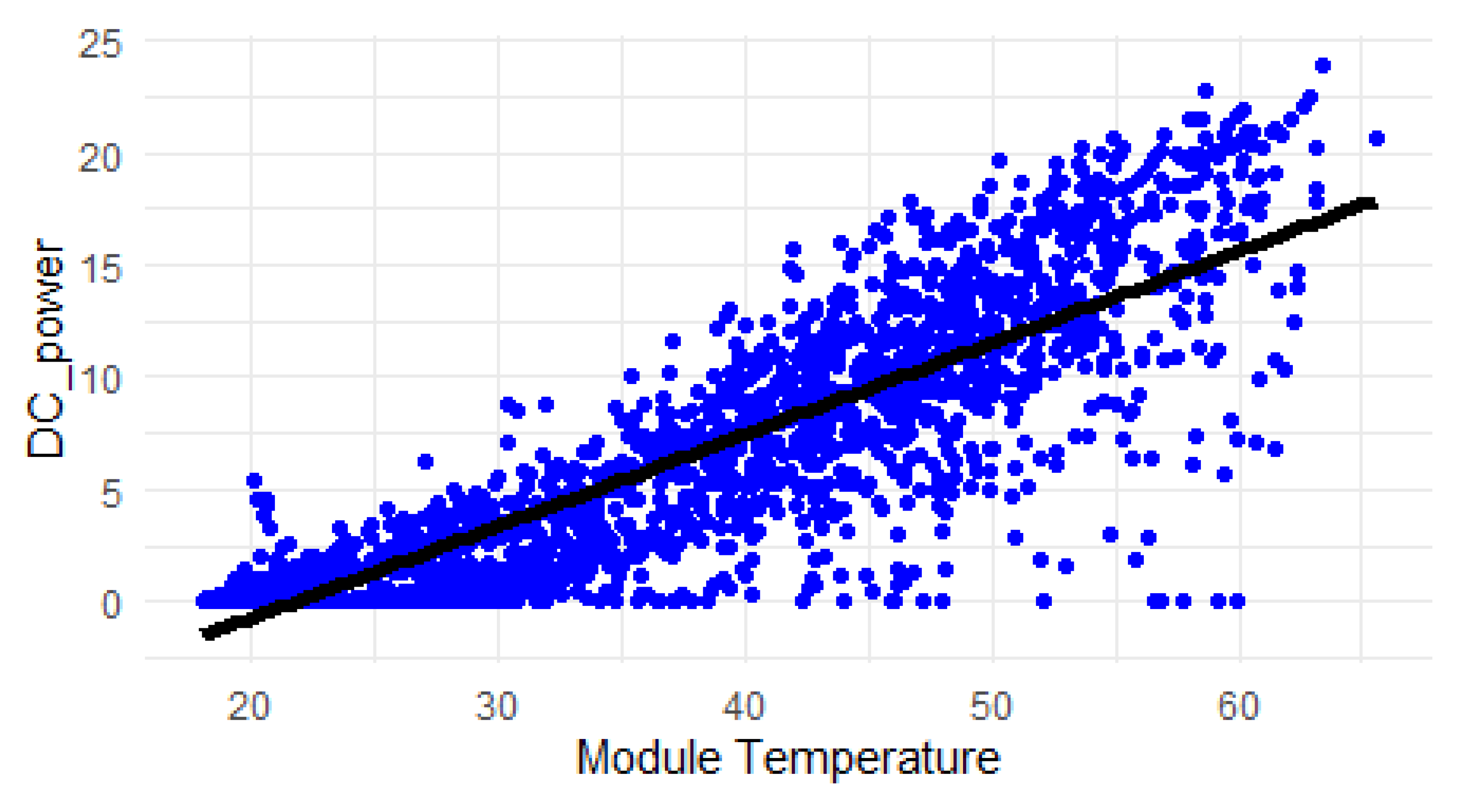
Figure 5.
Quadratic regression model.
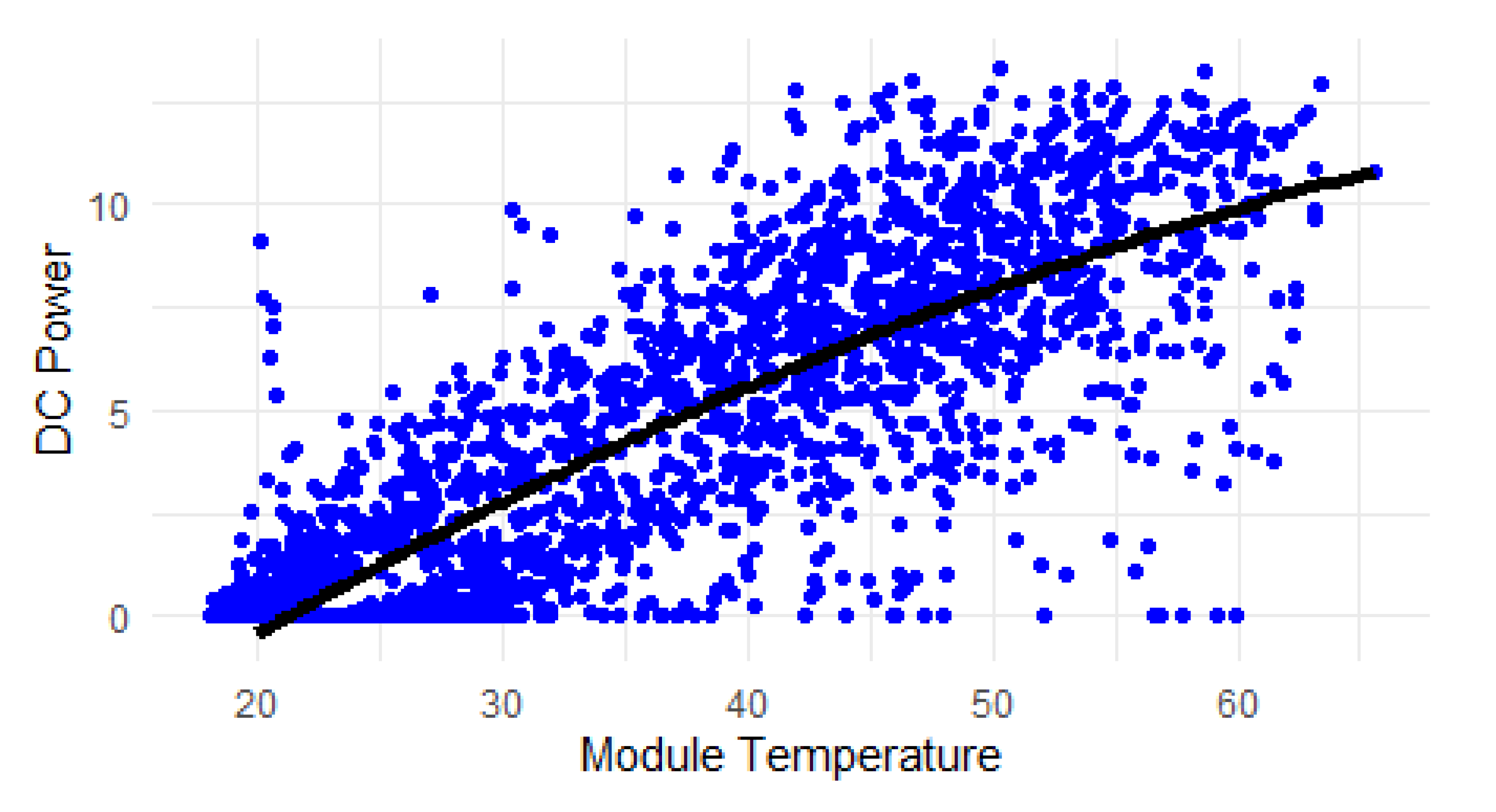
Figure 6.
Poisson regression model.
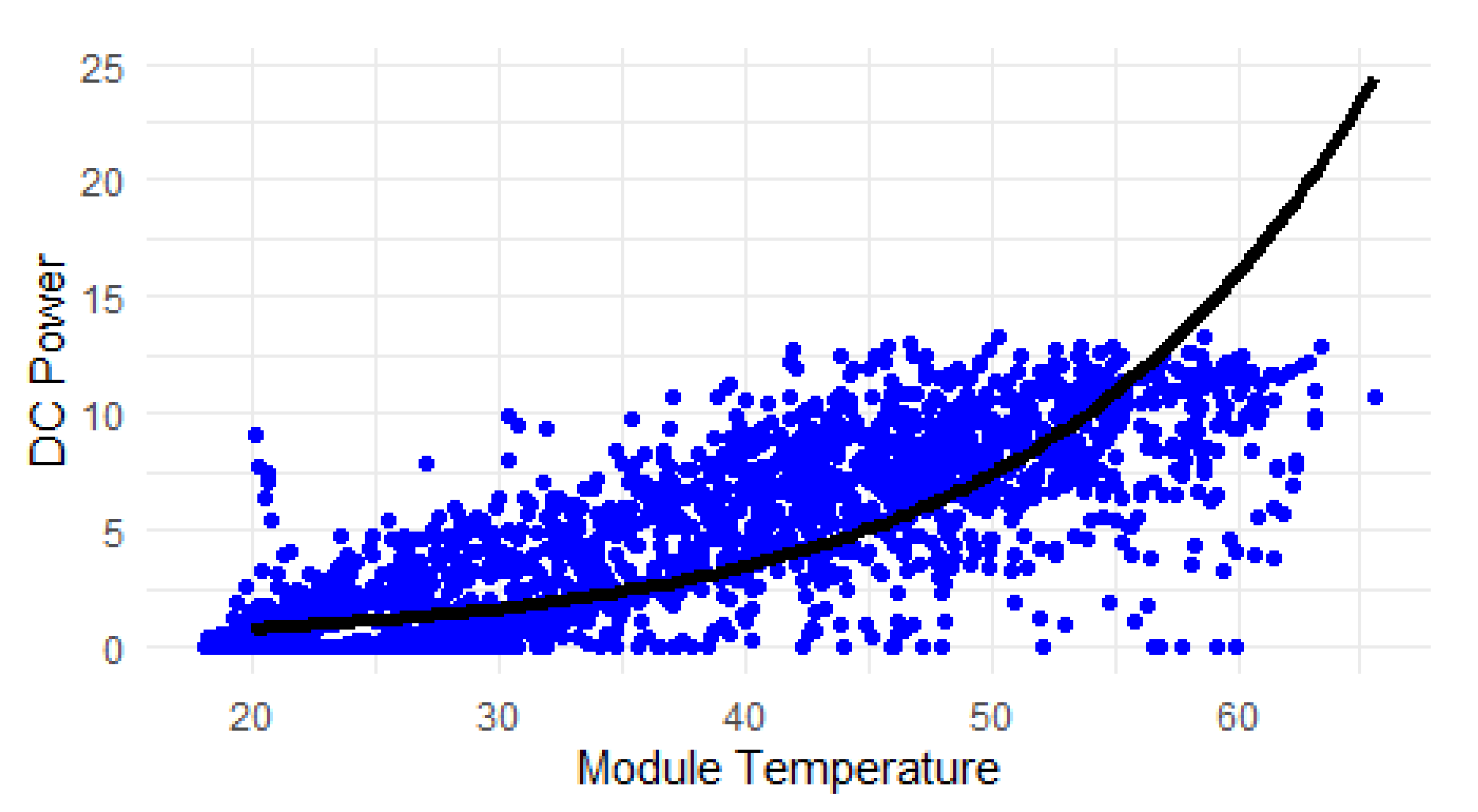
Figure 7.
Weibull model.
Figure 8.
Generalized linear model.
4.6. Analysis of Models
In this section, we compare the linear, quadratic, and Poisson regression models with the Weibull model, focusing on the provided estimates, standard errors, t-values, and p-values. Figure 9 presents the residuals, including minimum, 1Q, median, 3Q, and maximum values, which are essential for assessing the goodness of fit and the distribution of errors in the models.
Figure 10 displays the coefficients, including Estimate, Std. Error, t value, and Pr(), providing insights into the significance and impact of the predictor variables in the regression models.
The comparison sheds light on the suitability of each model for analyzing survival data and estimating reliability, particularly in the context of photovoltaic degradation. Additionally, we consider the implications of the model comparisons for understanding the behavior of systems over time and the estimation of hazard functions.
The findings indicate that the presence of negative values in linear and quadratic models suggests that they can predict outcomes falling below a certain baseline or threshold. In contrast, the Poisson model exhibits a narrower range and lower median, indicating a more conservative approach in its estimates, likely capturing the distribution of low-frequency events. Meanwhile, the Weibull model outputs entirely positive values, emphasizing the magnitude or duration of phenomena rather than their frequencies.
4.7. Regression Models: Residuals and Coefficients
When comparing regression models, it is important to consider their performance in terms of residuals. Residuals are the differences between the observed values and the predicted values from the regression model. By examining the distribution of residuals, we can assess how well the model fits the data and identify any patterns or discrepancies.
Based on the provided estimates, standard errors, t-values, and p-values, we can make some observations about the regression models and their relationship to photovoltaic degradation. However, it is important to note that without additional context or information about the specific variables and data used in the models, it is difficult to draw definitive conclusions.
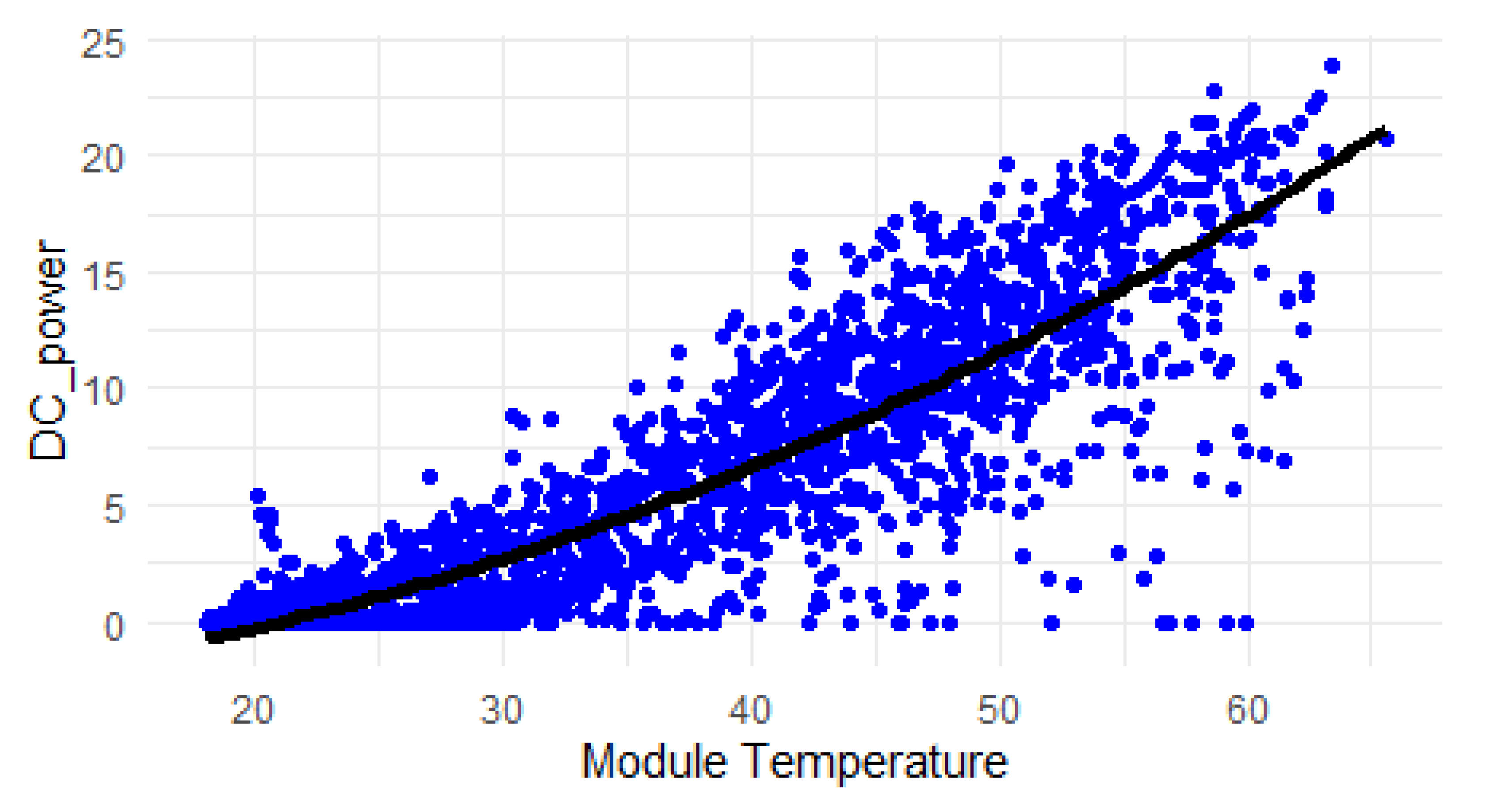
In the linear regression model, the positive estimate for the module temperature suggests that as the temperature increases, there is a positive effect on the response variable (possibly related to photovoltaic degradation). The p-value for the module temperature indicates that this effect is statistically significant at a certain level of significance.
The quadratic regression model does not show a significant relationship between the intercept and module temperature variables, as indicated by the high p-values. This suggests that the quadratic regression model may not be a good fit for explaining photovoltaic degradation based on the provided data.
The Poisson regression model shows a statistically significant relationship between the intercept and module temperature variables, as indicated by the p-values. A low p-value suggests that the relationship is unlikely to be due to chance.
The Weibull distribution, being a probability distribution rather than a regression model, provides estimates for the intercept and module temperature parameters. The estimates suggest a relationship between the variables. The statistically significant p-value for the module temperature indicates that this relationship is also likely not due to chance.
4.8. Weibull Model Compared to Regression
The Weibull model is commonly used in reliability analysis, including the analysis of photovoltaic degradation. It can be used to analyze the degradation of photovoltaic modules by estimating the failure rate or hazard function over time, providing insights into the reliability and lifetime of the modules.
Comparing minimum, 1st quartile, median, 3rd quartile, and maximum values, we can see that the Weibull distribution has significantly larger values compared to the regression models. The minimum value of the Weibull distribution is already larger than the maximum values of the regression models. The quartiles and median of the Weibull distribution are also much higher.
4.9. Three Types of Linear Models
In this section, we compare the linear, generalized, and hierarchical linear models. Similar to the basic models section, Figure 11 contains the residuals and Figure 12 presents the coefficients. These coefficients offer valuable insights into the significance and influence of the predictor variables incorporated within the regression models.
The analysis of the summary statistics for the linear models reveals that they yield identical results, suggesting that the choice of the model may not significantly impact the interpretation of the data in this case. This uniformity indicates that simpler models may suffice when the data does not exhibit complex relationships.
4.10. Comparing Basic Models to Advanced Models
The linear models show a significantly higher maximum residual compared to basic models, indicating that they may better capture the variability in the data. However, the presence of zeros in the minimum and first quartile suggests that these models may also be more robust in certain contexts, potentially reducing the impact of outliers.
While basic models provide a straightforward approach to regression analysis, they may struggle with complex datasets, as indicated by their wider range of residuals. In contrast, linear models offer enhanced flexibility and robustness, making them suitable for more intricate data relationships. The choice between these models should be guided by the specific characteristics of the data and the goals of the analysis.
4.11. Markov Chain Monte Carlo Models
The results from the MCMC RStan analysis provide a comprehensive view of the estimated parameters, namely alpha, beta, and sigma. Figure 13, Figure 14, Figure 15, Figure 16, and Figure 17 depict the mean parameter estimates and their associated standard errors across the various chains. These visualizations are essential for interpreting the reliability of the estimates and understanding the model’s performance, laying the groundwork for further inferential statistics and decision-making.
The MCMC RStan results shown in Figure 13 indicate that the parameter estimates for alpha, beta, and sigma are stable and precise across the different chains. The low standard errors and standard deviations, as shown in Figure 14, further support the reliability of these estimates. The visualizations created using ggplot2 provide a clear and effective means of communicating these findings.
Figure 15 provides clear evidence of the stability and reliability of the MCMC parameter estimates across the four chains. The consistent values for alpha, beta, and sigma, along with their low standard deviations, indicate that the MCMC process has performed effectively. This enables researchers to confidently use these parameter estimates for further analysis and decision-making processes in their modeling efforts.
The findings from Figure 16 indicate that both alpha and beta parameters are well estimated with high precision, while sigma and log posterior values provide important context regarding the model’s fit and reliability.
The stability and precision of these estimates reinforce confidence in the results derived from the MCMC sampling process, paving the way for further analysis or decision-making in the modeling efforts.
Figure 17 presents that while chains 1 and 2 exhibit longer warm-up durations, chains 3 and 4 show greater efficiency in processing, especially during the warm-up phase. This insight is crucial for refining MCMC configurations in future analyses, as it underscores the significance of tracking elapsed times to facilitate effective model fitting.
Figure 18 shows the elapsed time for MCMC brms.
Figure 19 provides an informative summary of the MCMC parameter estimates across different chains. The consistency in the alpha, beta, and sigma parameters suggests that the model is stable and reliable. The slight variations in the log posterior standard deviations across chains indicate some uncertainty, which is important for understanding the model’s fit.
Figure 20 provides clear evidence of the stability and reliability of the MCMC parameter estimates across the three parameters. The negative intercept suggests a significant baseline effect, while the estimates for DC Power and DC Power E2 indicate minimal to no effect. The convergence of the chains and the highly effective sample sizes further support the reliability of these estimates.
Figure 18 shows that while chains 1 and 2 show longer warm-up times, chains 3 and 4 demonstrate more efficient processing, particularly in the warm-up phase. This information could be valuable for optimizing MCMC configurations in future analyses, as it highlights the importance of monitoring elapsed times to ensure efficient model fitting. The stability and efficiency of the MCMC process are crucial for obtaining reliable estimates, and this plot effectively illustrates those dynamics.
The MCMC RStan results indicate that the parameter estimates for , , and are stable and precise across the different chains. The low standard errors and standard deviations further support the reliability of these estimates. The visualizations created using ggplot2 provide a clear and effective means of communicating these findings.
Figure 17 provides clear evidence of the stability and reliability of the MCMC parameter estimates across the four chains. The consistent values for , , and , along with their low standard deviations, indicate that the MCMC process has performed effectively. This enables researchers to confidently use these parameter estimates for further analysis and decision-making processes in their modeling efforts.
5. Comparing Usage of Different Libraries in R
By comparing the MCMC results from both RStan and brms, as shown in Figure 19, Figure 20, and Figure 18, we can draw deeper insights into the model’s efficacy and reliability, paving the way for informed conclusions and recommendations based on these findings, particularly in terms of model fitting, performance, and usability.
The standard errors of the mean for the chains in brms are generally larger than those in RStan, indicating that the RStan model may have more precise estimates for the parameters.
Both models report values close to 1.00, indicating good convergence. However, the brms model shows slightly higher Bulk and Tail Effective Sample Sizes (ESS), suggesting better mixing and more reliable estimates.
The brms model took significantly longer to run, with total sampling times ranging from 5.28 seconds to 10.791 seconds per chain. In contrast, the RStan model completed in about 2.365 seconds to 3.808 seconds per chain. This suggests that RStan may be more efficient for certain models, particularly when computational resources are limited.
The brms library for MCMC is designed to be user-friendly, allowing users to specify models using a formula syntax similar to that of base R functions. This makes it accessible for users who may not be familiar with the Stan programming language. RStan, while powerful, requires a deeper understanding of Stan’s syntax and model specification, which can be a barrier for some users.
Both packages leverage Stan’s robust MCMC algorithms, but brms offers a wider range of built-in distributions and link functions, making it suitable for a broader array of modeling scenarios.
5.1. Comparing Advanced Models to Previous Models
The AIC, BIC (Bayesian Information Criterion), and WAIC (Widely Applicable Information Criterion) metrics serve as critical tools for model evaluation [63], and Table 4 summarizes them because AIC is flexible and suitable for exploratory analyses, BIC is conservative and favors simpler models, and WAIC is robust for complex Bayesian models, making each criterion valuable in different modeling contexts.
Formulas for AIC, BIC and WAIC are calculated by formulas (1), (2) and (3)
where k is the number of parameters in the model, L is the maximum likelihood of the model, n is the number of observations in the dataset, is the posterior predictive distribution for the ith observation given the parameters and is the variance of the log of the posterior predictive distribution, which accounts for uncertainty in the predictions.
Table 4 summarizes the AIC, BIC, and WAIC values for different categories of models, including basic, linear, and advanced models. It highlights the performance of each model type, indicating which models yield the best fit based on these criteria.
Basic models generally provide better AIC values than linear and advanced models, suggesting they may be more suitable for the data. Basic models outperform linear and advanced models in terms of BIC, indicating they may be more appropriate for the dataset. Basic models again show superior WAIC values compared to linear and advanced models.
The analysis suggests that basic models, particularly the Weibull model, are not only more effective in fitting the data but also demonstrate a more appropriate balance of complexity and fit compared to linear and advanced models.
AIC is calculated using the formula, where k is the number of parameters in the model and L is the likelihood of the model [44]. AIC is best used in exploratory analyses where capturing the best fit is crucial, particularly in smaller datasets where the risk of overfitting is lower [18]. The penalty for complexity in AIC is moderate, allowing for a balance between model fit and complexity [26]. It encourages the inclusion of additional parameters if they significantly improve the model’s likelihood.
BIC is ideal for situations where simplicity is prioritized to avoid overfitting and enhance interpretability [58]. The term increases the penalty for complexity as the sample size grows, making BIC more conservative in model selection [34]. BIC imposes a high penalty for complexity, particularly in larger datasets, which discourages the use of overly complex models [28]. This makes it more stringent than AIC in terms of model selection.
WAIC is calculated using the formula, where represents the posterior predictive distribution [70]. This approach focuses on the model’s predictive performance rather than just the likelihood.
The penalty for complexity in WAIC is variable and depends on the model’s predictive accuracy [61]. It adapts to the model’s ability to generalize to new data, making it less rigid than AIC and BIC. WAIC is most effective in evaluating complex Bayesian models, particularly hierarchical structures, by providing a robust measure of predictive performance while accounting for parameter uncertainty [71].
Figure 21 shows informative criteria values for each kind of model. The consistently lower values for basic models suggest they effectively balance these aspects.
MCMC models provide a robust framework for evaluating model fit through AIC, BIC, and WAIC. While basic and linear models may yield lower values for these criteria in certain contexts, MCMC allows for a more nuanced assessment of model performance by incorporating the entire posterior distribution of parameters.
AIC values range from 1545.032 (Weibull) to Inf (Poisson regression), indicating that the Weibull model performs best among basic models. AIC values are significantly higher for linear models, with all models around 14195.6, suggesting a poorer fit than basic models. MCMC RStan has an extremely high AIC of 33531673, indicating a very poor fit.
BIC values also show the Weibull model as the best performer (1556.42), while the Poisson model is not applicable (Inf). BIC values are consistently high (around 14219.82) for linear models, indicating a poor fit relative to basic models. MCMC RStan’s BIC is similarly high (33531697), reinforcing its poor fit.
WAIC values indicate the Weibull model (1543.032) as the best, while the Poisson model is not applicable (Inf). WAIC values are consistent with AIC and BIC, showing high values around 14193.6 for linear models. WAIC for MCMC RStan is not provided, but the high AIC and BIC suggest a poor fit.
Linear models rely heavily on assumptions such as normality of residuals and homoscedasticity. MCMC models, on the other hand, are less sensitive to these assumptions, making them more robust in various scenarios. This robustness can result in more reliable AIC, BIC, and WAIC values, as MCMC models can still perform well even when the data do not meet the stringent assumptions required by linear models.
MCMC models can accommodate complex and hierarchical structures that basic and linear models may struggle to represent. This flexibility allows MCMC to model non-linear relationships and interactions more effectively, which can lead to better-fit metrics. Although basic models may show lower AIC, BIC, and WAIC values, they often do so at the expense of oversimplifying the underlying data structure. MCMC’s ability to model complexity can ultimately lead to more accurate predictions and insights.
The evaluation of model performance through AIC, BIC, and WAIC metrics reveals that the Weibull model consistently demonstrates superior fit among basic models, making it the most reliable choice for analysis. In contrast, both linear models and advanced models like MCMC RStan exhibit significantly poorer fits, as evidenced by their elevated AIC and BIC values.
This analysis underscores the necessity of careful model selection, as choosing a model with a better fit can greatly enhance the validity and reliability of statistical findings. Ultimately, the results advocate for prioritizing the Weibull model in future analyses while exercising caution with more complex models that do not provide a better fit.
6. Model Performance Comparison
The Weibull model is the top performer among basic models, showing the best fit across AIC, BIC, and WAIC metrics. Linear models demonstrate significantly poorer fits compared to basic models, with consistently high AIC and BIC values.
The MCMC RStan model has extremely high AIC and BIC values, indicating a very poor fit and highlighting the need for caution in using advanced models that do not improve upon basic models.
Basic models are more effective than linear models, indicating that simpler models may be more appropriate for the data. They are favored over advanced models, indicating that simpler approaches may yield better results.
Table 5 comprehensively compare various statistical models based on their performance metrics. The models are categorized into three groups: Basic Models, Linear Models, and Advanced Models. Each table highlights the fit of these models to the dataset, providing insights into their effectiveness and suitability for analysis. The conclusions drawn from these comparisons will guide researchers in selecting the most appropriate modeling approach for their data.
There is little distinction in performance between linear and advanced models, indicating a need to reevaluate model choice. While basic models may provide lower AIC, BIC, and WAIC values in some cases, MCMC models offer significant advantages in terms of flexibility, robustness, uncertainty quantification, and predictive performance.
These benefits make MCMC a powerful tool for model selection and evaluation, particularly in complex datasets where traditional models may fall short. Therefore, despite the current findings favoring simpler models, the potential of MCMC models should not be overlooked, especially in scenarios where a deeper understanding of the data is required.
7. Conclusions
The paper provides a comparison of Bayesian models used for degradation modeling in photovoltaic systems. It has yielded several significant findings regarding the analysis of regression models and their implications for understanding the relationship between DC power and response variables.
The significance of DC power varies across different regression models, with notable effects in Linear and Weibull models, but not in the Quadratic model. This suggests that model choice is critical in interpreting results. The analysis of residuals reveals distinct distributions across models; the Poisson model has lower medians and a narrower range compared to Linear and Quadratic models, which include negative values. This highlights the importance of model selection based on data characteristics. In medium-advanced models, linear models produced identical results, indicating that simpler models may be sufficient when data relationships are not complex.
The GLM and HGLM models introduced a significant quadratic effect, suggesting more complex relationships than the linear model, underscoring the need for model complexity based on data behavior. The MCMC RStan results show stable and precise parameter estimates across different chains, with low standard errors, reinforcing the reliability of these estimates for further analysis.
The use of plots to illustrate regression results and residual distributions enhances comprehension and facilitates a better understanding of model behavior. The article provides a thorough comparison of basic and linear models, showcasing the implications of model choice on interpreting relationships within data.
The evaluation of MCMC chains for both RStan and brms models offers valuable insights into the performance and reliability of Bayesian analysis techniques. By highlighting the significance of model choice, the article contributes practical guidance for researchers in selecting appropriate models based on their data’s characteristics. The findings contribute to a methodological framework for analyzing regression models, emphasizing the need to consider both complexity and the underlying data characteristics.
Future research could explore other regression models beyond those analyzed, such as mixed-effects models, to assess their performance and significance of DC power. Investigating the findings with larger and more diverse datasets could provide insights into model robustness and generalizability across different contexts. The predictive modeling approach presented here complements recent studies on energy consumption forecasting in complex infrastructures [82]. Our predictive model yields accurate estimates of failure rates under operational conditions. Yet, translating predictions into actionable strategies requires system-level integration. Similar integrated approaches of forecasting plus decision support have been demonstrated in domains such as budget planning, marrying time-series methods and BI tools to assist operational decisions [83].
Future studies could focus on optimizing MCMC configurations further by analyzing elapsed times and efficiency across various datasets to enhance model fitting processes. Additionally, future research could delve deeper into non-linear relationships and interactions between variables, utilizing more complex models to uncover hidden patterns in the data.
Incorporating machine learning techniques alongside traditional statistical models could enhance predictive performance and allow for more nuanced analyses of complex relationships in data.
Author Contributions
Conceptualization, A.J.-K. and J.B.; Methodology, A.J.-K.; Software, A.J.-K.; Validation, A.J.-K. and J.B.; Formal Analysis, A.J.-K.; Investigation, A.J.-K.; Resources, J.B.; Data Curation, A.J.-K.; Writing—Original Draft Preparation, A.J.-K.; Writing—Review and Editing, J.B.; Visualization, A.J.-K.; Supervision, J.B.; Project Administration, J.B. All authors have read and agreed to the published version of the manuscript..
Funding
Work of Anna Jarosz and Jerzy Baranowski partially realised in the scope of project titled ”Process Fault Prediction and Detection”. Project was financed by The National Science Centre on the base of decision no. UMO-2021/41/B/ST7/03851. Part of work was funded by AGH’s Research University Excellence Initiative under project “DUDU – Diagnostyka Uszkodzeń i Degradacji Urzadzeń”.
Institutional Review Board Statement
Not applicable.
Informed Consent Statement
Not applicable.
Data Availability Statement
Data comes from Pythonafroz’s Kaggle notebook titled “Solar Power Generation Data”. The information and metrics derived from this resource were instrumental in shaping our model. Additionally, Annajarosz96 made all the models accessible in the GitHub repository. These models provided a robust foundation for our research and experimentation.
Acknowledgments
Authors would like to thank Dr Marta Zagorowska for her great help in manuscript consultation. Authors would also like to express their gratitude to Dr. Khaled Laadjal for extending invitation to submit the article. During the preparation of this manuscript, authors used ChatGPT 5 for the purposes of style verification and refinement. The authors have reviewed and edited the output and take full responsibility for the content of this publication.
Conflicts of Interest
The authors declare no conflicts of interest.
Abbreviations
The following abbreviations are used in this manuscript:
| PV | Photovoltaic |
| AIC | Akaike Information Criterion |
| BIC | Bayesian Information Criterion |
| WAIC | Widely Applicable Information Criterion |
| MCMC | Markov Chain Monte Carlo |
| HMM | Hidden Markov Model |
| GLM | Generalized Linear Model |
| HGLM | Hierarchical Generalized Linear Model |
| brms | Bayesian Regression Models using Stan |
| RStan | R Interface to Stan for Bayesian Inference |
| DC | Direct Current |
| AC | Alternating Current |
| ESS | Effective Sample Size |
| IRT | Infrared Thermography |
| APC | Article Processing Charge |
References
- Paci, B.; Righi Riva, F.; Generosi, A.; Distler, A.; Egelhaaf, H.J. Semitransparent Organic Photovoltaic Devices: Interface/Bulk Properties and Stability Issues. Nanomaterials 2024, 14, 269. [Google Scholar] [CrossRef]
- Ebrahim, E.A.; Cengiz, M.A.; Terzi, E. The Best Fit Bayesian Hierarchical Generalized Linear Model Selection Using Information Complexity Criteria in the MCMC Approach. Journal of Mathematics 2024, 1459524. [Google Scholar] [CrossRef]
- Akcaoğlu, S.C.; Martinopoulos, G.; Koidis, C.; Kiymaz, D.; Zafer, C. Investigation of cell-level potential-induced degradation mechanisms on perovskite, dye-sensitized and organic photovoltaics. Solar Energy 2019, 190, 301–318. [Google Scholar] [CrossRef]
- Baranowski, J.; Grobler-Dębska, K.; Kucharska, E. Recognizing vsc dc cable fault types using bayesian functional data depth. Energies 2021, 14. [Google Scholar] [CrossRef]
- Abbas, M.; Zeng, L.; Guo, F.; Yuan, X.C.; Cai, B. A critical review on crystal growth techniques for scalable deposition of photovoltaic perovskite thin films. Materials 2020, 13, 4851. [Google Scholar] [CrossRef]
- Kucharska, E. Heuristic method for decision-making in common scheduling problems. Applied Sciences (Switzerland) 2017, 7. [Google Scholar] [CrossRef]
- Torki, Z.; Benhamida, M.; Haddad, Z.; Chouder, A.; Brahimi, I. Effects of Temperature and Solar Radiation on Photovoltaic Modules Performances Installed in Oued Keberit Power Plant, Algeria. Journal of Advanced Research in Fluid Mechanics and Thermal Sciences 2023, 112, 204–216. [Google Scholar] [CrossRef]
- Amani, K.M.; Hili, O.; Kouakou, K.J.G. Statistical inference in marginalized zero-inflated Poisson regression models with missing data in covariates. Math Methods Stat. 2023, 32, 241–259. [Google Scholar] [CrossRef]
- Xi, Z.; Jing, R.; Lee, C.; Hayrapetyan, M. Recent research on battery diagnostics, prognostics, and uncertainty management. In Advances in Battery Manufacturing, Services, and Management Systems; 2016; pp. 175–216.
- Malvoni, M.; Kumar, N.M.; Chopra, S.S.; Hatziargyriou, N. Connected solar photovoltaic power plant in tropical semi-arid environment of India. Solar Energy 2020, 203, 101–113. [Google Scholar] [CrossRef]
- Kirk, B.P.; Alghamdi, A.R.; Griffith, M.J.; Andersson, G.G.; Andersson, M.R. Investigation of different degradation pathways for organic photovoltaics at different temperatures. Materials Advances 2024, 5, 4438–4451. [Google Scholar] [CrossRef]
- Rana, H.; Pandit, B.; Sivakumar Babu, G.L. Estimation of Uncertainties in Soil Using MCMC Simulation and Effect of Model Uncertainty. Geotechnical and Geological Engineering 2023, 41, 4415–4429. [Google Scholar] [CrossRef]
- Son, C.K.; Kim, J.M. Bayes linear estimator for two-stage and stratified randomized response models. Model Assisted Statistics and Applications 2015, 10, 321–333. [Google Scholar] [CrossRef]
- Alshanbari, H.M.; Odhah, O.H.; Al-Mofleh, H.; Khosa, S.K.; El-Bagoury, A.A.A.H. A new flexible Weibull extension model: Different estimation methods and modeling an extreme value data. Heliyon 2023, 9, e21704. [Google Scholar] [CrossRef] [PubMed]
- Xie, F.; Czogalla, O.; Shi, H. Application of Lithium-Ion Battery Thermal Management System in Electric Vehicle Simulation. In Lecture Notes in Intelligent Transportation and Infrastructure, Part F1389; 2021; pp. 135–147.
- Mahalakshmi, K.; Reddy, K.S.; Subrahmanyam, A. Outdoor degradation evaluation of multi-junction solar cell for four Fresnel concentrated photovoltaic systems. International Journal of Sustainable Energy 2022, 41, 1958–1972. [Google Scholar] [CrossRef]
- Flottemesch, T.J.; Gordon, B.D.; Jones, S.S. Advanced Statistics: Developing a Formal Model of Emergency Department Census and Defining Operational Efficiency. Academic Emergency Medicine 2007, 14, 799–809. [Google Scholar] [CrossRef]
- Kaplanis, S.; Kaplani, E.; Kaldellis, J.K. PV Temperature Prediction Incorporating the Effect of Humidity and Cooling Due to Seawater Flow and Evaporation on Modules Simulating Floating PV Conditions. Energies 2023, 16, 4756. [Google Scholar] [CrossRef]
- Zhou, Q.; Man, J.; Son, J. Data-driven prognostics for batteries subject to hard failure. In Advances in Battery Manufacturing, Services, and Management Systems; 2016; pp. 233–254.
- Rajput, P.; Malvoni, M.; Kumar, N.M.; Sastry, O.S.; Tiwari, G.N. Risk priority number for understanding the severity of photovoltaic failure modes and their impacts on performance degradation. Case Studies in Thermal Engineering 2019, 16, 100563. [Google Scholar] [CrossRef]
- Abdelhadi, S.; Elbahnasy, K.; Abdelsalam, M. A proposed model to predict auto insurance claims using machine learning techniques. Journal of Theoretical and Applied Information Technology 2020, 98, 3428–3437. [Google Scholar]
- Shively, T.S.; Walker, S.G. Miscellanea: On Bayes factors for the linear model. Biometrika 2018, 105, 739–744. [Google Scholar] [CrossRef]
- Maruyama, Y.; Strawderman, W.E. Improved robust Bayes estimators of the error variance in linear models. Journal of Statistical Planning and Inference 2013, 143, 1091–1097. [Google Scholar] [CrossRef]
- Dhimish, M.; Kettle, J. Impact of solar cell cracks caused during potential-induced degradation (PID) tests. IEEE Transactions on Electron Devices 2022, 69, 604–612. [Google Scholar] [CrossRef]
- Feng, P.; Li, L.; Yang, Y.; Zhang, Q.; Xu, Z. Effect of Thermal Cycling Aging Photovoltaic Ribbon on the Electrical Performance of Photovoltaic Modules. IEEE Journal of Photovoltaics 2024, 14, 149–159. [Google Scholar] [CrossRef]
- Dhimish, M.; Chen, Z. Novel Open-Circuit Photovoltaic Bypass Diode Fault Detection Algorithm. IEEE Journal of Photovoltaics 2019, 9, 1819–1827. [Google Scholar] [CrossRef]
- Gayathri, K.; Chitra, M. An efficient predictive and diagnosis model using Bayes shared information criterion based on associative classifier. International Journal of Applied Engineering Research 2015, 10, 19077–19096. [Google Scholar] [CrossRef]
- Gomaa, M.R.; Ahmed, M.; Rezk, H. Temperature distribution modeling of PV and cooling water PV/T collectors through thin and thick cooling cross-fined channel box. Energy Reports 2022, 8, 1144–1153. [Google Scholar] [CrossRef]
- Liu, P.; Huang, Y.; Wang, Z.; He, Z.; Wu, H. Evolution of interfacial defects and energy losses during aging of organic photovoltaics. Physica B: Condensed Matter 2024, 677, 415707. [Google Scholar] [CrossRef]
- Poddar, S.; Rougieux, F.; Evans, J.P.; Prasad, A.A.; Bremner, S.P. Accelerated degradation of photovoltaic modules under a future warmer climate. Progress in Photovoltaics: Research and Applications 2024, 32, 456–467. [Google Scholar] [CrossRef]
- García, E.; Ponluisa, N.; Quiles, E.; Zotovic-Stanisic, R.; Gutiérrez, S.C. Solar Panels String Predictive and Parametric Fault Diagnosis Using Low-Cost Sensors. Sensors 2022, 22, 332. [Google Scholar] [CrossRef]
- Lillo-Sánchez, L.; López-Lara, G.; Vera-Medina, J.; Pérez-Aparicio, E.; Lillo-Bravo, I. Degradation analysis of photovoltaic modules after operating for 22 years. A case The study with comparisons. Solar Energy 2021, 222, 84–94. [Google Scholar] [CrossRef]
- Meena, R.; Kumar, M.; Kumar, S.; Gupta, R. Comparative degradation analysis of accelerated-aged and field-aged crystalline silicon photovoltaic modules under Indian subtropical climatic conditions. Results in Engineering 2022, 16, 100674. [Google Scholar] [CrossRef]
- Atia, D.M.; Hassan, A.A.; El-Madany, H.T.; Eliwa, A.Y.; Zahran, M.B. Degradation and energy performance evaluation of mono-crystalline photovoltaic modules in Egypt. Scientific Reports 2023, 13, 13066. [Google Scholar] [CrossRef]
- Hossion, A.; Manoj Kumar, N.; Bajaj, M.; Elnaggar, M.F.; Kamel, S. Analysis of various degradations of five years aged mono c-Si, poly c-Si, and thin-film photovoltaic modules from rooftop solar installations in Dhaka’s tropical wet and dry climate conditions. Frontiers in Energy Research 2023, 11, 996176. [Google Scholar] [CrossRef]
- Hacke, P.; Spataru, S.; Habersberger, B.; Chen, Y. Field-representative evaluation of POTENTIAL-INDUCED DEGRADATION-polarization in TOPCon PV modules by accelerated stress testing. Progress in Photovoltaics: Research and Applications 2024, 32, 346–355. [Google Scholar] [CrossRef]
- Portet, S. A primer on model selection using the Akaike Information Criterion. Infectious Disease Modelling 2020, 5, 111–128. [Google Scholar] [CrossRef]
- Eldeghady, G.S.; Kamal, H.A.; Moustafa Hassan, M.A. Comparative analysis of the performance of supervised learning algorithms for photovoltaic system fault diagnosis. Science and Technology for Energy Transition (STET) 2024, 79. [Google Scholar] [CrossRef]
- Jamil, W.J.; Rahman, H.A.; Baharin, K.A. Experiment-based The study on the impact of soiling on PV system’s performance. International Journal of Electrical and Computer Engineering 2016, 6, 810–818. [Google Scholar] [CrossRef]
- Mandai, K.; Miao, S.; Dowaki, K. Environmental impact assessment on polymer electrolyte fuel cell co-generation system, lithium-ion battery, and photovoltaic hybrid system combination and operation, considering performance degradation. Cleaner Engineering and Technology 2024, 20, 100756. [Google Scholar] [CrossRef]
- Ochoa, J.; García, E.; Quiles, E.; Correcher, A. Redundant fault diagnosis for photovoltaic systems based on an IRT low-cost sensor. Sensors 2023, 23, 1314. [Google Scholar] [CrossRef]
- Kumar, N.M.; Malvoni, M. A preliminary The study of the degradation of large-scale c-Si photovoltaic system under four years of operation in semi-arid climates. Results in Physics 2019, 12, 1395–1397. [Google Scholar] [CrossRef]
- Premkumar, M.; Jangir, P.; Elavarasan, R.M.; Sowmya, R. Opposition decided gradient-based optimizer with balance analysis and diversity maintenance for parameter identification of solar photovoltaic models. Journal of Ambient Intelligence and Humanized Computing 2023, 14, 7109–7131. [Google Scholar] [CrossRef]
- Chang, L.; Zhou, Z.; Chen, Y.; Liao, T.; Tan, X. Akaike Information Criterion-based conjunctive belief rule base learning for complex system modeling. Knowledge-Based Systems 2018, 161, 47–64. [Google Scholar] [CrossRef]
- Wang, Y.; Guo, J.; Qi, Y.; Lian, J.; Yin, X. Research Progress on Deep Learning Based Defect Detection Technology for Solar Panels. EAI Endorsed Transactions on Energy Web 2024, 11, 1–8. [Google Scholar] [CrossRef]
- Hamada, T.; Azuma, T.; Nanno, I.; Fujii, M.; Oke, S. Impact of Bypass Diode Fault Resistance Values on Burnout in Bypass Diode Failures in Simulated Photovoltaic Modules with Various Output Parameters. Energies 2023, 16, 5879. [Google Scholar] [CrossRef]
- Mononen, T. A case The study of the widely applicable Bayesian information criterion and its optimality. Statistics and Computing 2015, 25, 929–940. [Google Scholar] [CrossRef]
- García, E.; Quiles, E.; Zotovic-Stanisic, R.; Gutiérrez, S.C. Predictive Fault Diagnosis for Ship Photovoltaic Modules Systems Applications. Sensors 2022, 22, 2175. [Google Scholar] [CrossRef]
- Kurzweil, P.; Brandt, K. Overview of rechargeable lithium battery systems. In Electrochemical Power Sources: Fundamentals, Systems, and Applications Li-Battery Safety; 2018; pp. 47–82.
- Li, X.; Xia, X.; Zhang, Z. Poisson subsampling-based estimation for growing-dimensional expectile regression in massive data. Statistics and Computing 2024, 34, 133. [Google Scholar] [CrossRef]
- Oozeki, T.; Yamada, T.; Kato, K.; Yamamoto, T. An analysis of reliability for photovoltaic systems on the field test project for photovoltaic in Japan. In Proceedings of the ISES Solar World Congress 2007, 2007, pp. 1628–1632. 2007; 2007, 1628. [Google Scholar] [CrossRef]
- Wang, L.; Pettit, L. Linear Bayes estimators applied to the inverse Gaussian lifetime model. Journal of Systems Science and Complexity 2016, 29, 1683–1692. [Google Scholar] [CrossRef]
- Markevich, V.P.; Vaqueiro-Contreras, M.; De Guzman, J.T.; Murin, L.I.; Peaker, A.R. Boron–Oxygen Complex Responsible for Light-Induced Degradation in Silicon Photovoltaic Cells: A New Insight into the Problem. Physica Status Solidi (A) Applications and Materials Science 2019, 216, 1900315. [Google Scholar] [CrossRef]
- Radaideh, M.I.; Borowiec, K.; Kozlowski, T. Integrated framework for model assessment and advanced uncertainty quantification of nuclear computer codes under Bayesian statistics. Reliability Engineering and System Safety 2019, 189, 357–377. [Google Scholar] [CrossRef]
- Sato, R.; Ishii, T.; Choi, S.; Kasu, M.; Masuda, A. Output power behavior of passivated emitter and rear cell photovoltaic modules during early installation stage: Influence of light-induced degradation. Japanese Journal of Applied Physics 2019, 58, 106510. [Google Scholar] [CrossRef]
- Xie, Q.; Peng, D.L. Rational Material Design and Performance Optimization of Transition Metal Oxide-Based Lithium Ion Battery Anodes. Advanced Battery Materials 2019, 159–208. [Google Scholar]
- Aragon, B.; Cawse-Nicholson, K.; Hulley, G.; Houborg, R.; Fisher, J. K-sharp: A segmented regression approach for image sharpening and normalization. Science of Remote Sensing 2023, 8, 100095. [Google Scholar] [CrossRef]
- Sharma, M.K. Alternative designs and technological advancements of phase change material integrated photovoltaics: A state-of-the-art review. Journal of Energy Storage 2022, 48, 104020. [Google Scholar] [CrossRef]
- Cavanaugh, J.E.; Neath, A.A. The Akaike information criterion: Background, derivation, properties, application, interpretation, and refinements. Wiley Interdisciplinary Reviews: Computational Statistics 2019, 11, e1460. [Google Scholar] [CrossRef]
- Han, W.; Zhang, L.; Han, Y. Mathematical modeling, performance analysis and control of battery equalization systems: Review and recent developments. In Advances in Battery Manufacturing, Services, and Management Systems; 2016; pp. 281–302.
- Müller, J.W. High-efficient, cost-effective, and reliable silicon solar cells and modules in mass production. In Springer Series in Optical Sciences; 2020; pp. 95–112. [CrossRef]
- Friel, N.; McKeone, J.P.; Oates, C.J.; Pettitt, A.N. Investigation of the widely applicable Bayesian information criterion. Statistics and Computing 2017, 27, 833–844. [Google Scholar] [CrossRef]
- Tina, G.M.; Ventura, C.; Scavo, F.B. Technological and design solutions for enhancement of photovoltaic producibility. In Recent Advances in Renewable Energy Technologies: Volume 1; 2021; pp. 91–148. [CrossRef]
- Belhaouas, N.; Hafdaoui, H.; Hadjrioua, F.; Chahtou, A.; Mehareb, F. Failures and performance of different aged PV modules operated under northern Algerian climate conditions: Analysis, assessment, and recommended solutions. Engineering Failure Analysis 2024, 163, 108504. [Google Scholar] [CrossRef]
- Zhou, Y. Polymer Composites for Electrical Engineering; 2021; pp. 1–27.
- Bar, H.Y.; Booth, J.G.; Wells, M.T. A Scalable Empirical Bayes Approach to Variable Selection in Generalized Linear Models. Journal of Computational and Graphical Statistics 2020, 29, 535–546. [Google Scholar] [CrossRef]
- Yang, H.; Lu, W. Graphene-based electrochemical microsupercapacitors for miniaturized energy storage applications. In NanoScience and Technology; 2016; pp. 271–291.
- Wilson, A.L.; Goldstein, M.; Dent, C.J. Varying Coefficient Models and Design Choice for Bayes Linear Emulation of Complex Computer Models with Limited Model Evaluations. SIAM-ASA Journal on Uncertainty Quantification 2022, 10, 350–378. [Google Scholar] [CrossRef]
- Zanesco, I.; Moehlecke, A.; Ferronato, J.; Leite, B.I.D.S.R.; Policarpi, T.C. Influence of Passivation and Solar Cell Configuration on the Electrical Parameter Degradation of Photovoltaic Modules. Energies 2024, 17, 832. [Google Scholar] [CrossRef]
- Wong, J.; Lim, Y.S. Revolution of energy storage system in smart grids. In Renewable and Alternative Energy: Concepts, Methodologies, Tools, and Applications; 2016; pp. 1669–1694.
- Gao, C.; van der Vaart, A.W.; Zhou, H.H. A general framework for Bayes structured linear models. Annals of Statistics 2020, 48, 2848–2878. [Google Scholar] [CrossRef]
- Zhou, X.; Liu, Z. Applications of graphene in lithium ion batteries. In Graphene: Energy Storage and Conversion Applications; 2014; pp. 65–136.
- York, M.; Larson, K.; Harris, K.C.; Ragones, H.; Golodnitsky, D. Solid batteries chemistries beyond lithium. In Sustainable Energy Storage in the Scope of Circular Economy: Advanced Materials and Device Design; 2023; pp. 69–122.
- Zhang, H.; Gao, Z.; Du, C.; Cui, Y.; Shen, X. Parameter estimation of three-parameter Weibull probability model based on outlier detection. RSC Advances 2022, 12, 34154–34164. [Google Scholar] [CrossRef]
- Zang, X. Graphene-based flexible energy storage devices. In Graphene: Fabrication, Characterizations, Properties and Applications; 2017; pp. 175–199.
- Yoshino, M.; Kameda, T.; Watanabe, H.; Yamada, M. Development of Highly-Efficient Energy Storage System Using Soled Oxide Electrolysis Cell. In Ceramic for Energy Conversion, Storage, and Distribution Systems; 2016; Vol. 255, pp. 101–111.
- Wu, G.; Liu, T.; Hu, M.; Chen, R.; Xing, G. Crystallinity and Phase Control in Formamidinium-Based Dion–Jacobson 2D Perovskite via Seed-Induced Growth for Efficient Photovoltaics. Advanced Materials 2023, 35, 2303061. [Google Scholar] [CrossRef] [PubMed]
- Wang, F.; Zhai, Z.; Zhao, Z.; Di, Y.; Chen, X. Physics-informed neural network for lithium-ion battery degradation stable modeling and prognosis. Nature Communications 2024, 15, 4332. [Google Scholar] [CrossRef] [PubMed]
- Kaggle. Solar Power Generation Data. https://www.kaggle.com/datasets/anikannal/solar-power-generation-data?resource=download. Accessed: 2023-06.
- Verma, S.; Yadav, D.K. Recent research and developments of degradation assessment and its diagnosis methods for solar PV plant: a review. International Journal of Applied Power Engineering 2024, 13, 483–498. [Google Scholar] [CrossRef]
- Selig, K.; Shaw, P.; Ankerst, D. Bayesian information criterion approximations to Bayes factors for univariate and multivariate logistic regression models. International Journal of Biostatistics 2021, 17, 241–266. [Google Scholar] [CrossRef] [PubMed]
- Kawa, K.; Mularczyk, R.; Bauer, W.; Grobler-Dębska, K.; Kucharska, E. Prediction of Energy Consumption on Example of Heterogenic Commercial Buildings. Energies 2024, 17. [Google Scholar] [CrossRef]
- Grobler-Dębska, K.; Mularczyk, R.; Gawęda, B.; Kucharska, E. Time Series Methods and Business Intelligent Tools for Budget Planning—Case Study. Applied Sciences 2025, 15. [Google Scholar] [CrossRef]
Figure 1.
Model of a photovoltaic system.
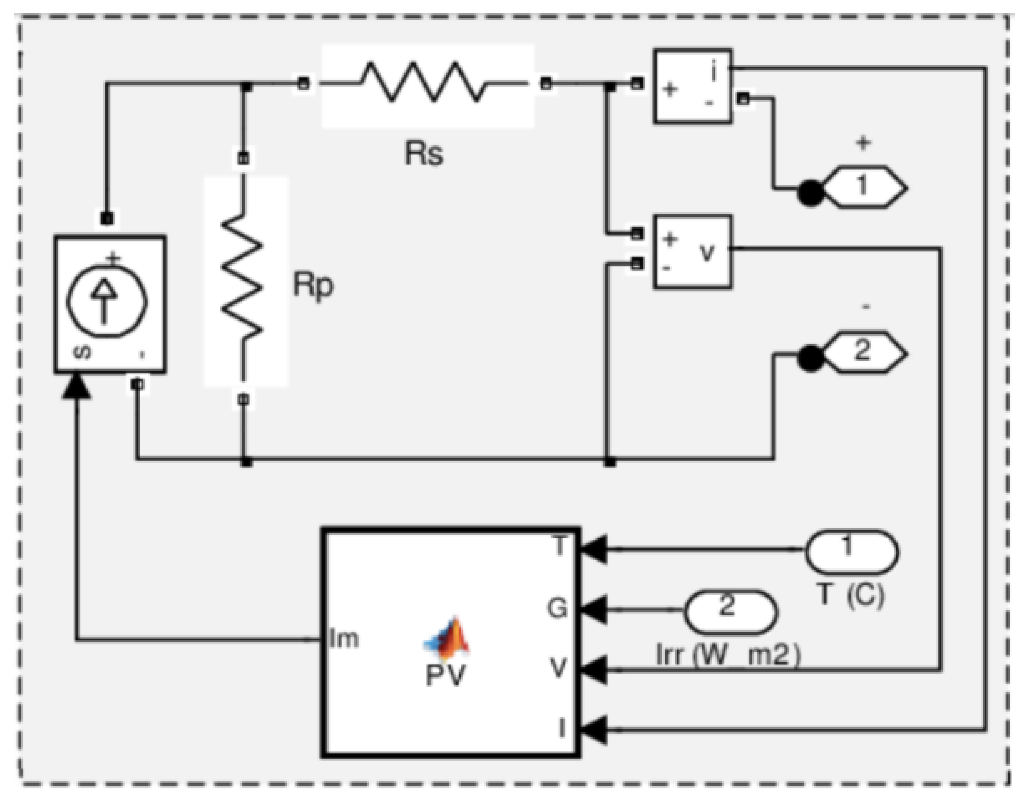
Figure 2.
DC and AC power outcome.
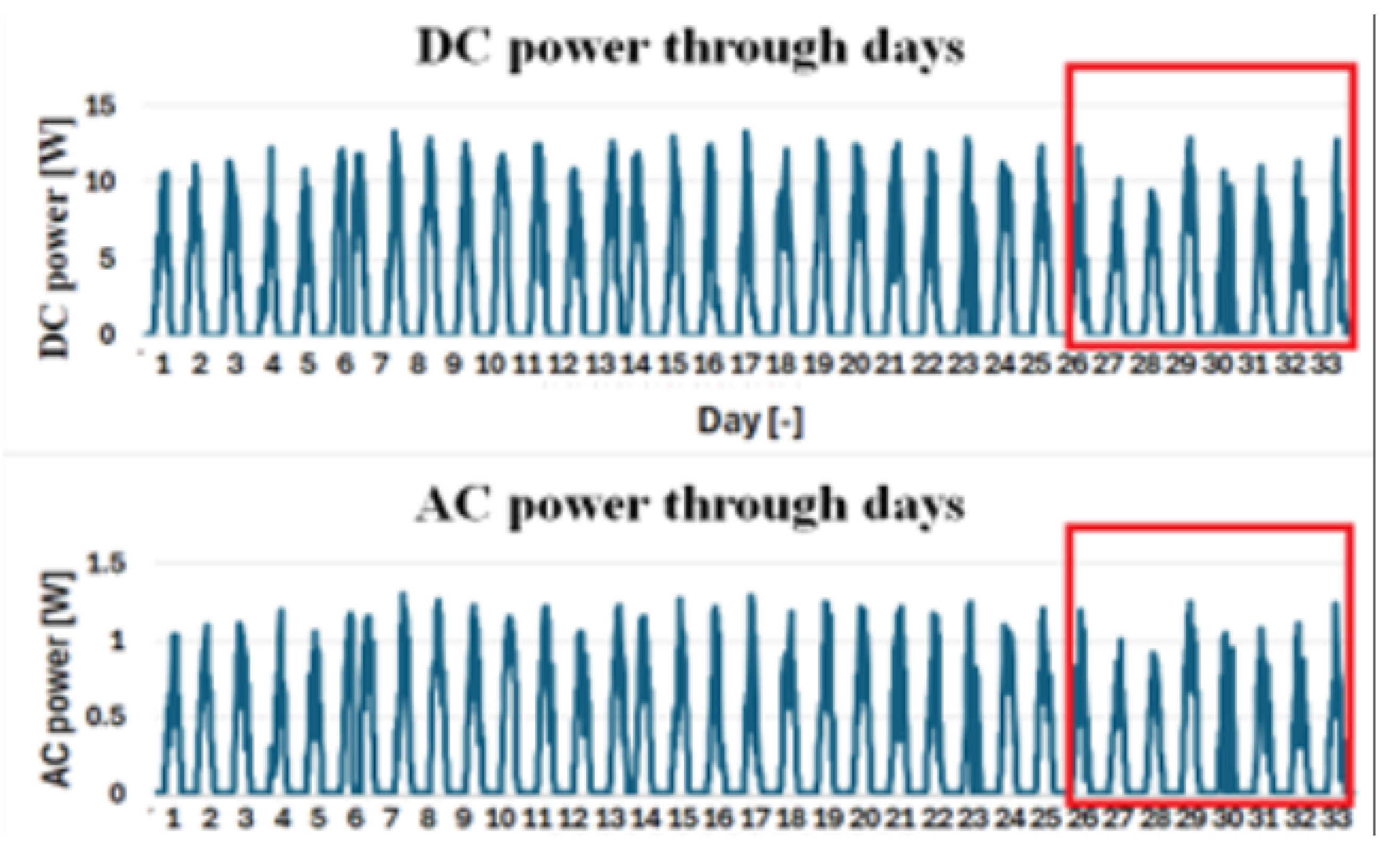
Figure 3.
Module and ambient temperature with irradiation.
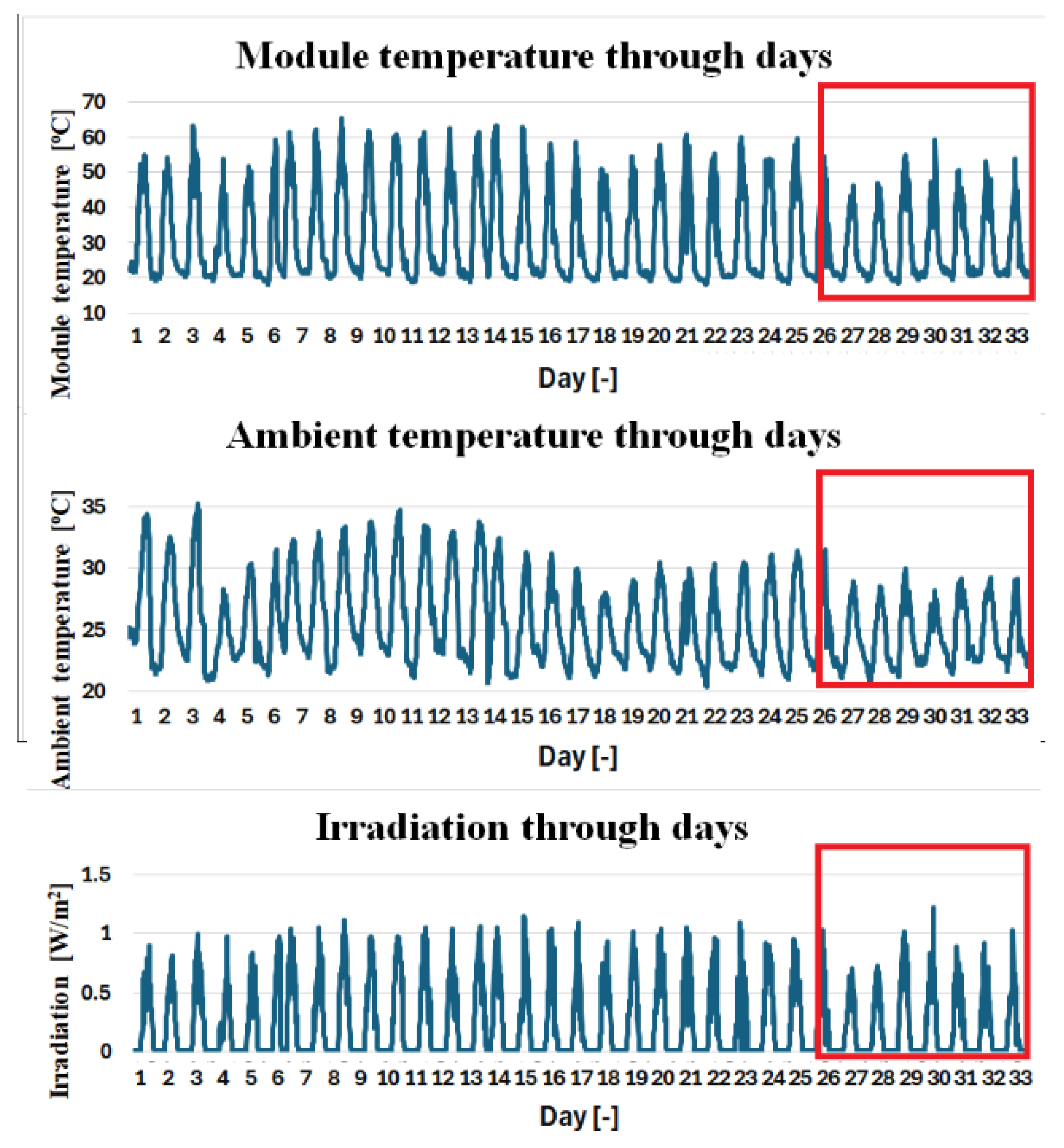
Figure 9.
Residual analysis in basic models.
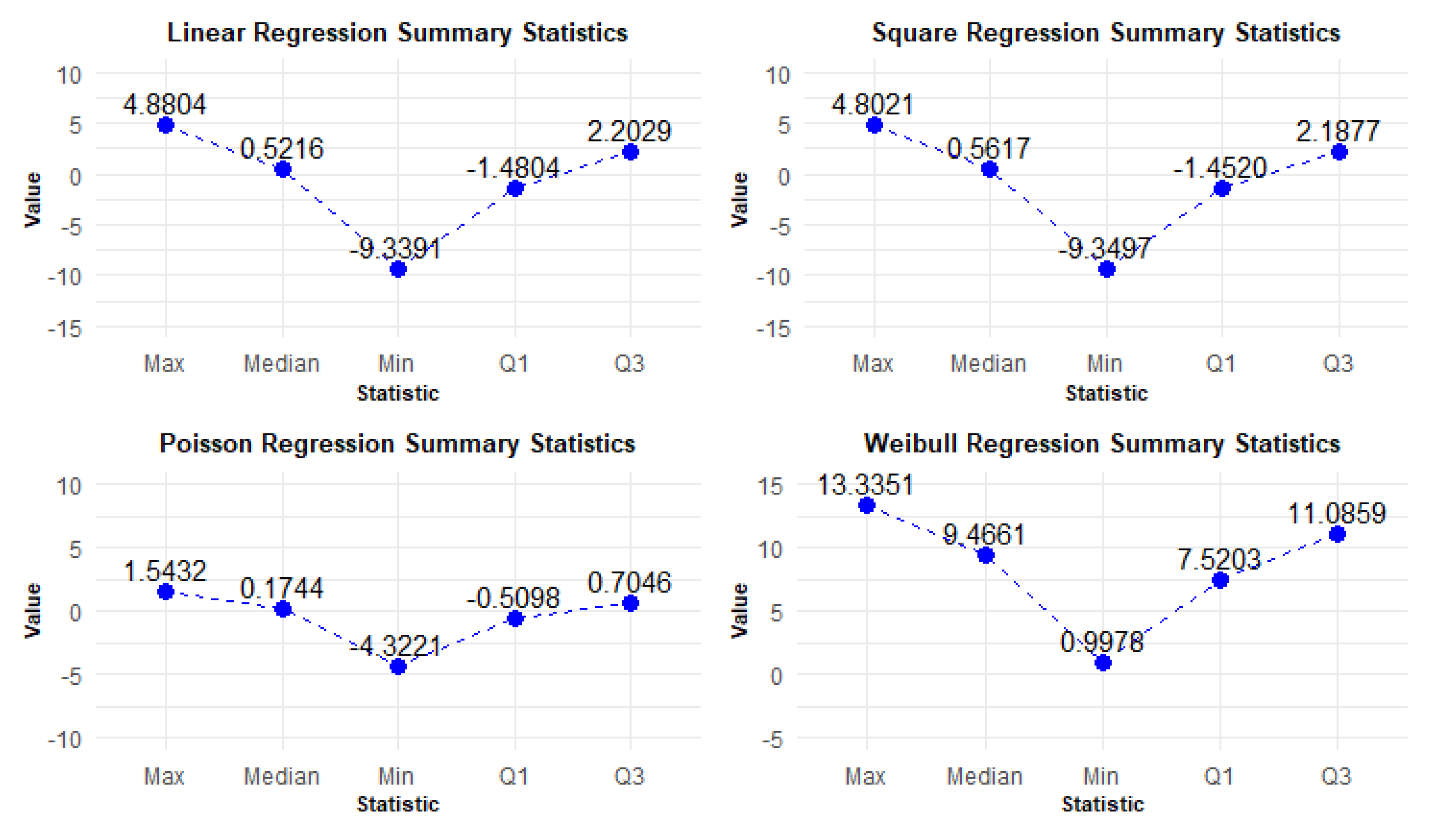
Figure 10.
Coefficient analysis in basic models.
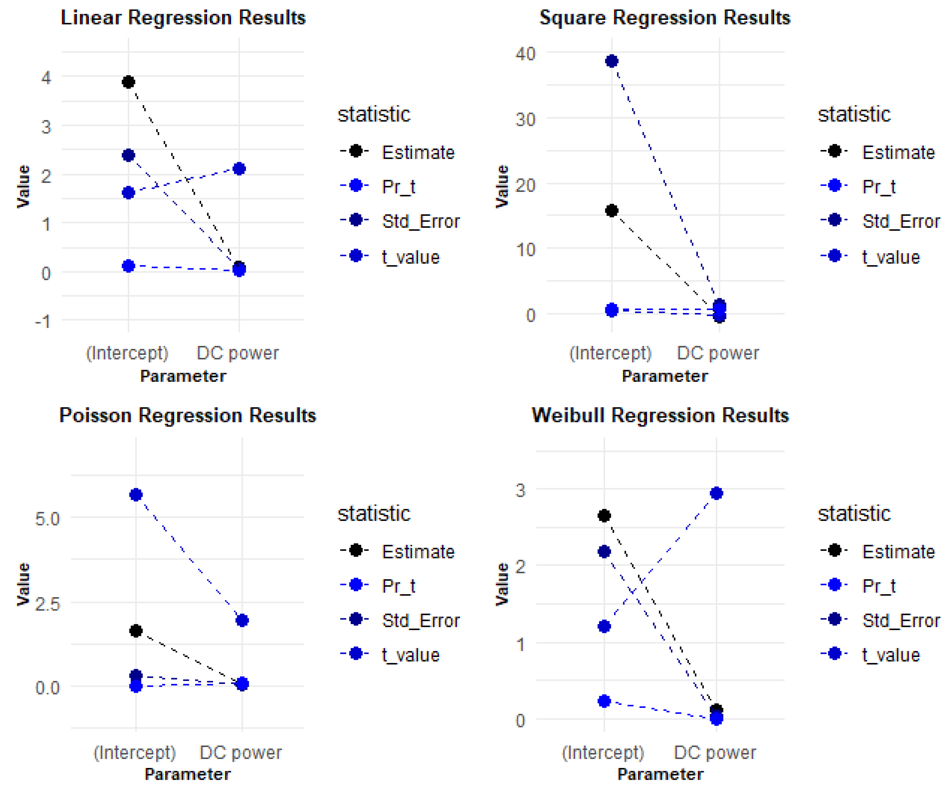
Figure 11.
Residual analysis in linear models.
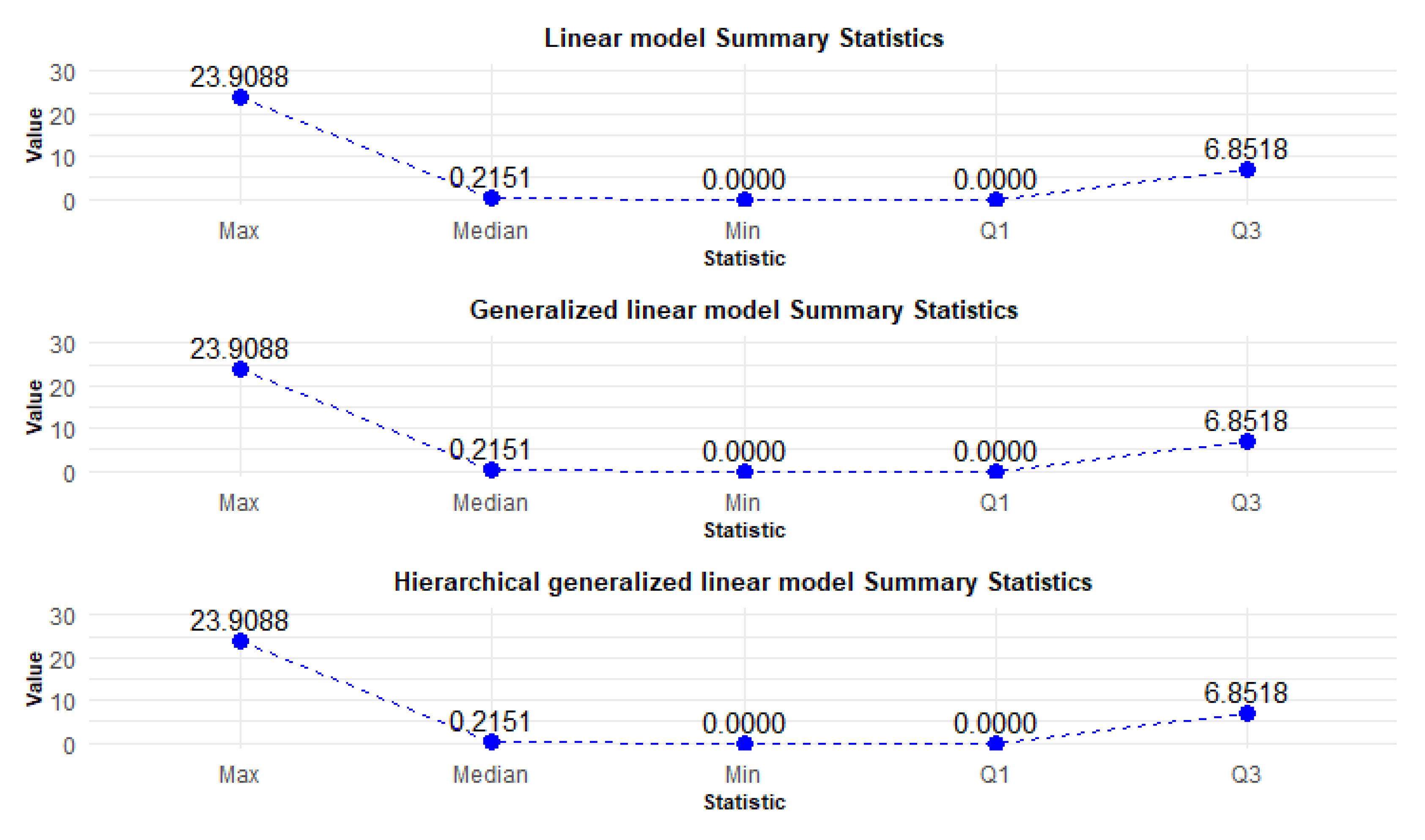
Figure 12.
Coefficient analysis in linear models.
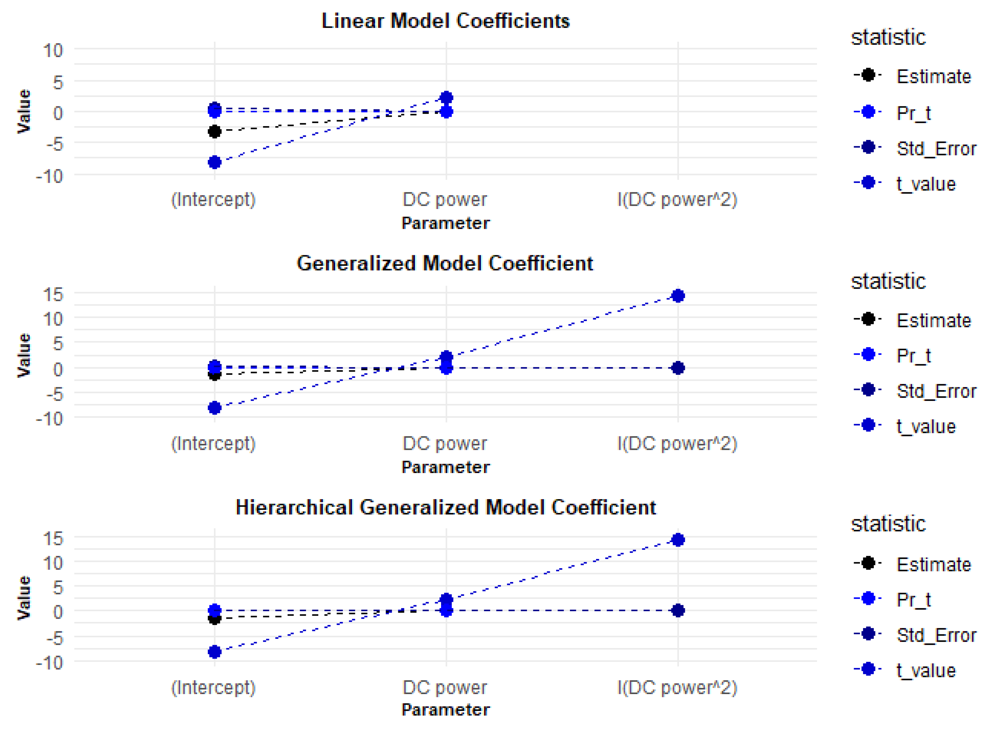
Figure 13.
MCMC parameter estimates (chain 1).
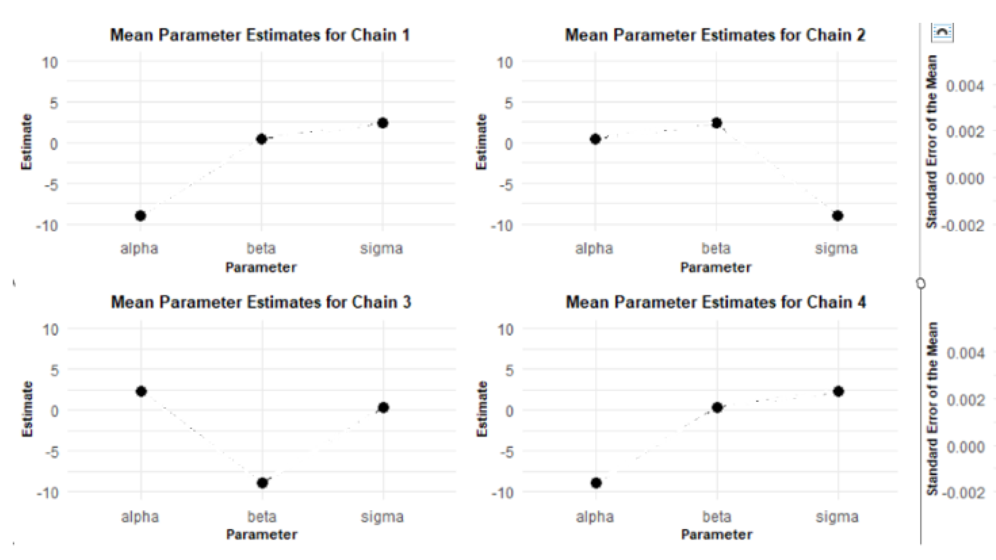
Figure 14.
Standard Error for MCMC RStan.
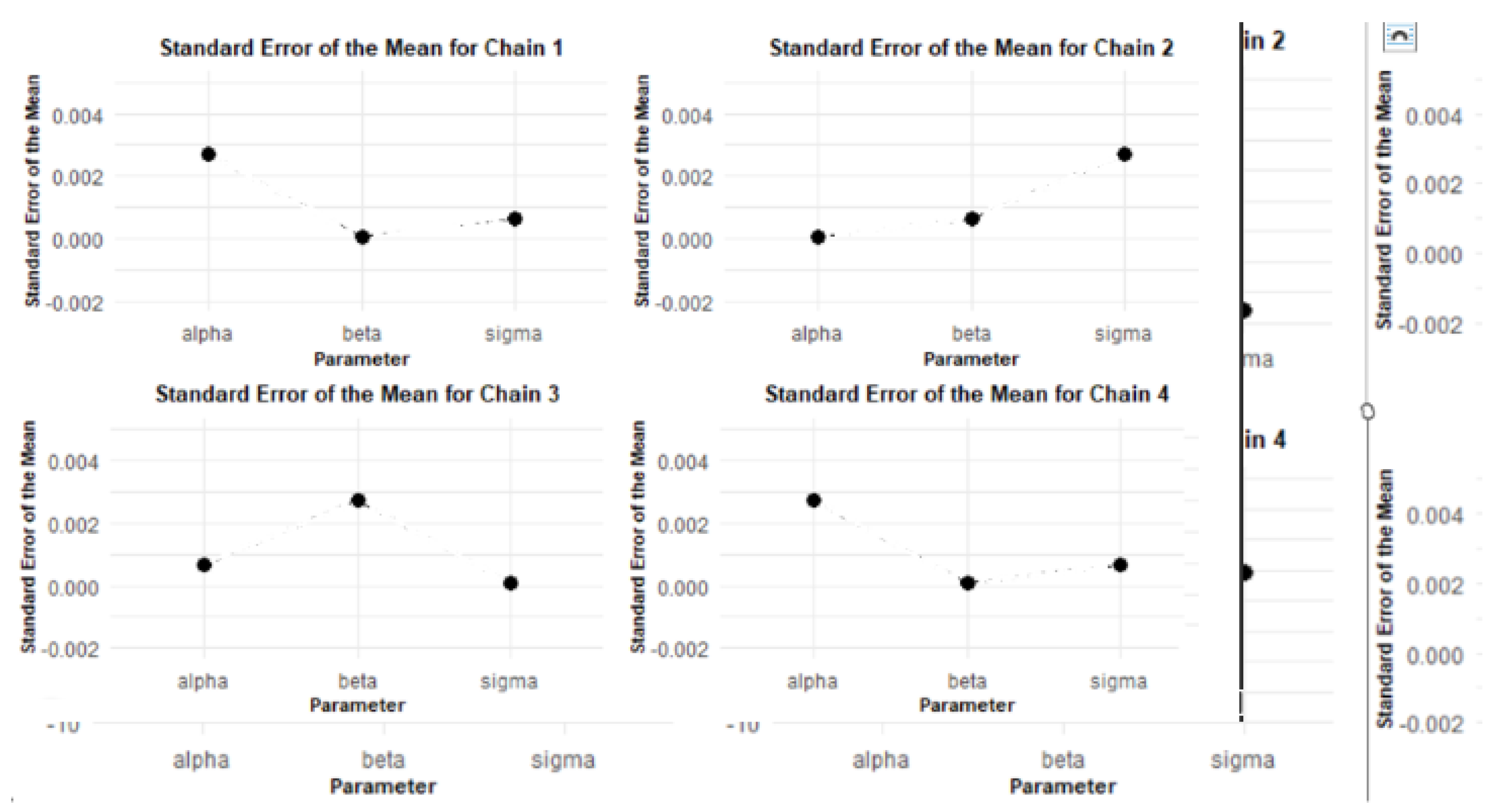
Figure 15.
MCMC RStan Parameters Values.
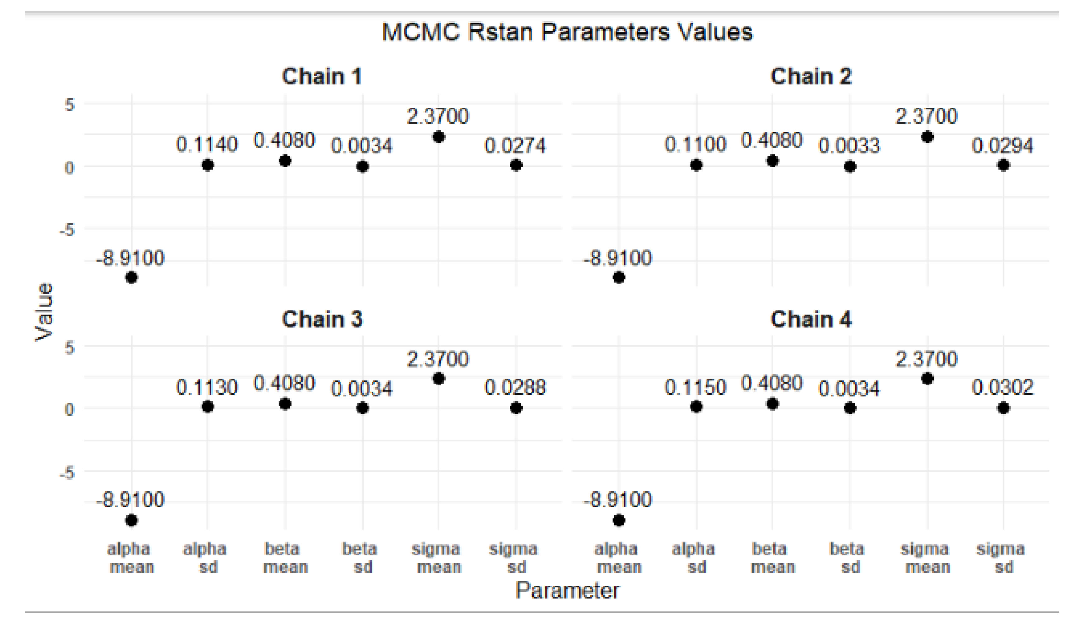
Figure 16.
Estimates for MCMC RStan Parameters.
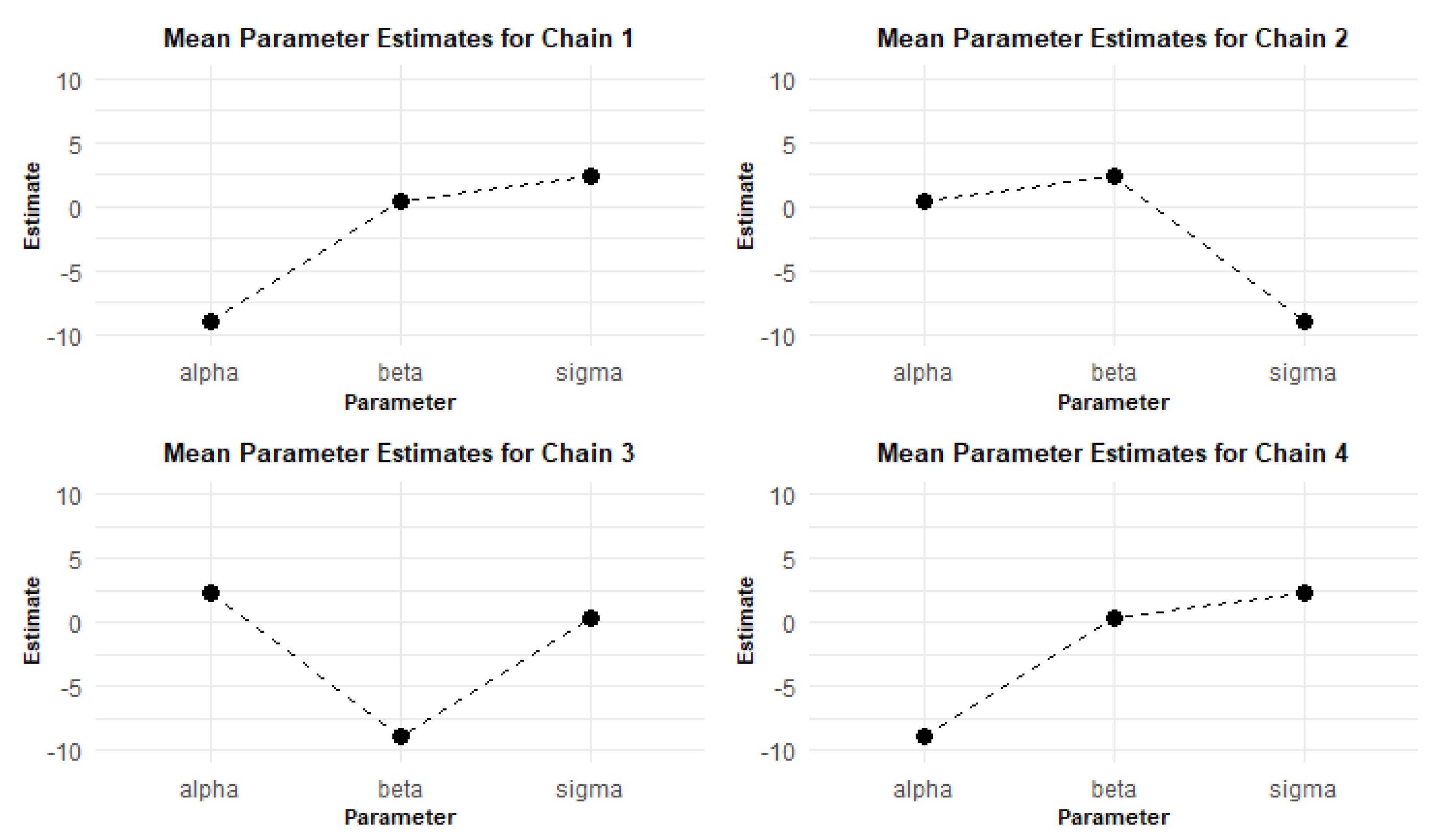
Figure 17.
Elapsed Time for MCMC RStan.
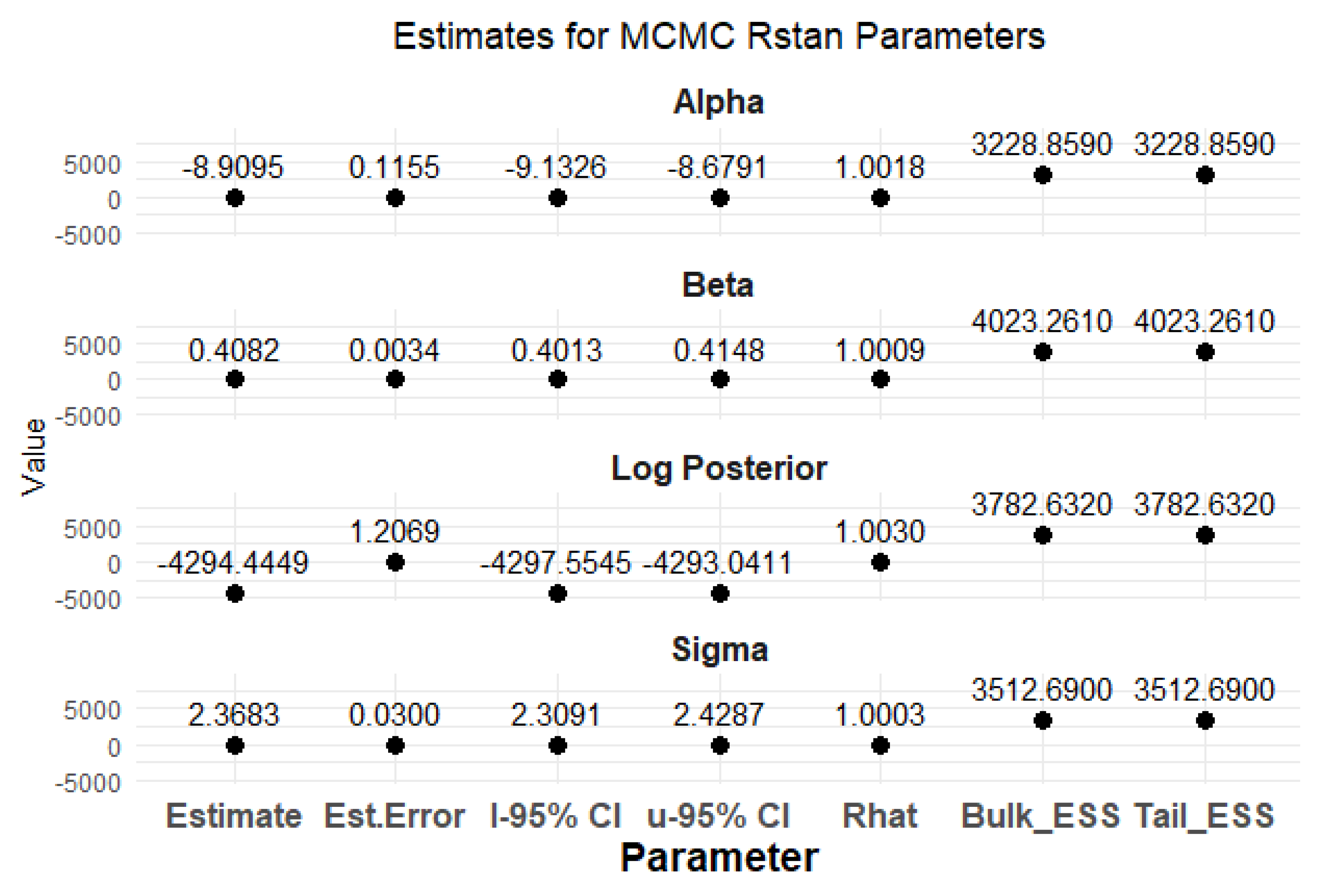
Figure 18.
Elapsed Time for MCMC brms.
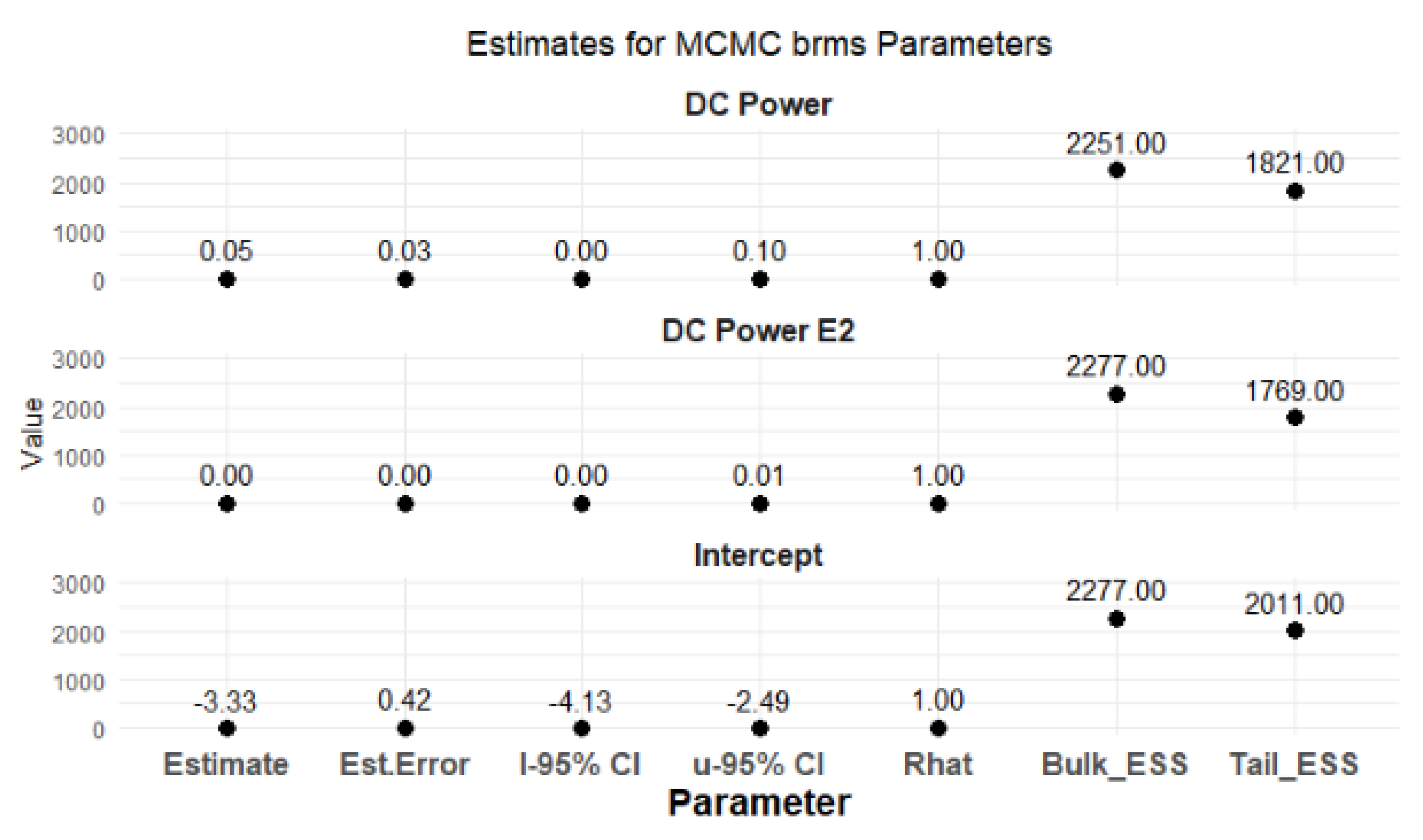
Figure 19.
MCMC brms Parameters Values.
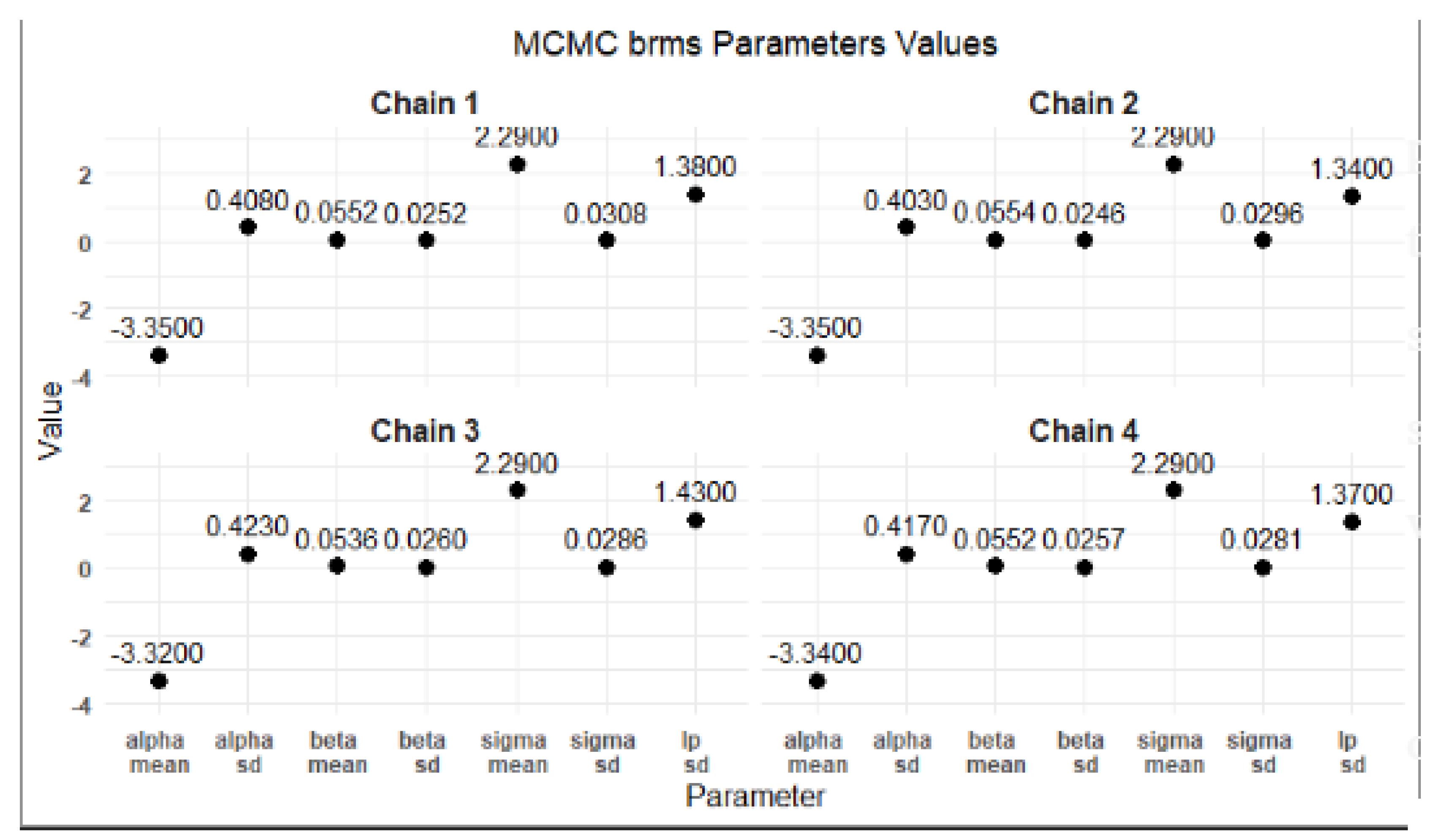
Figure 20.
Estimates for MCMC brms Parameters.
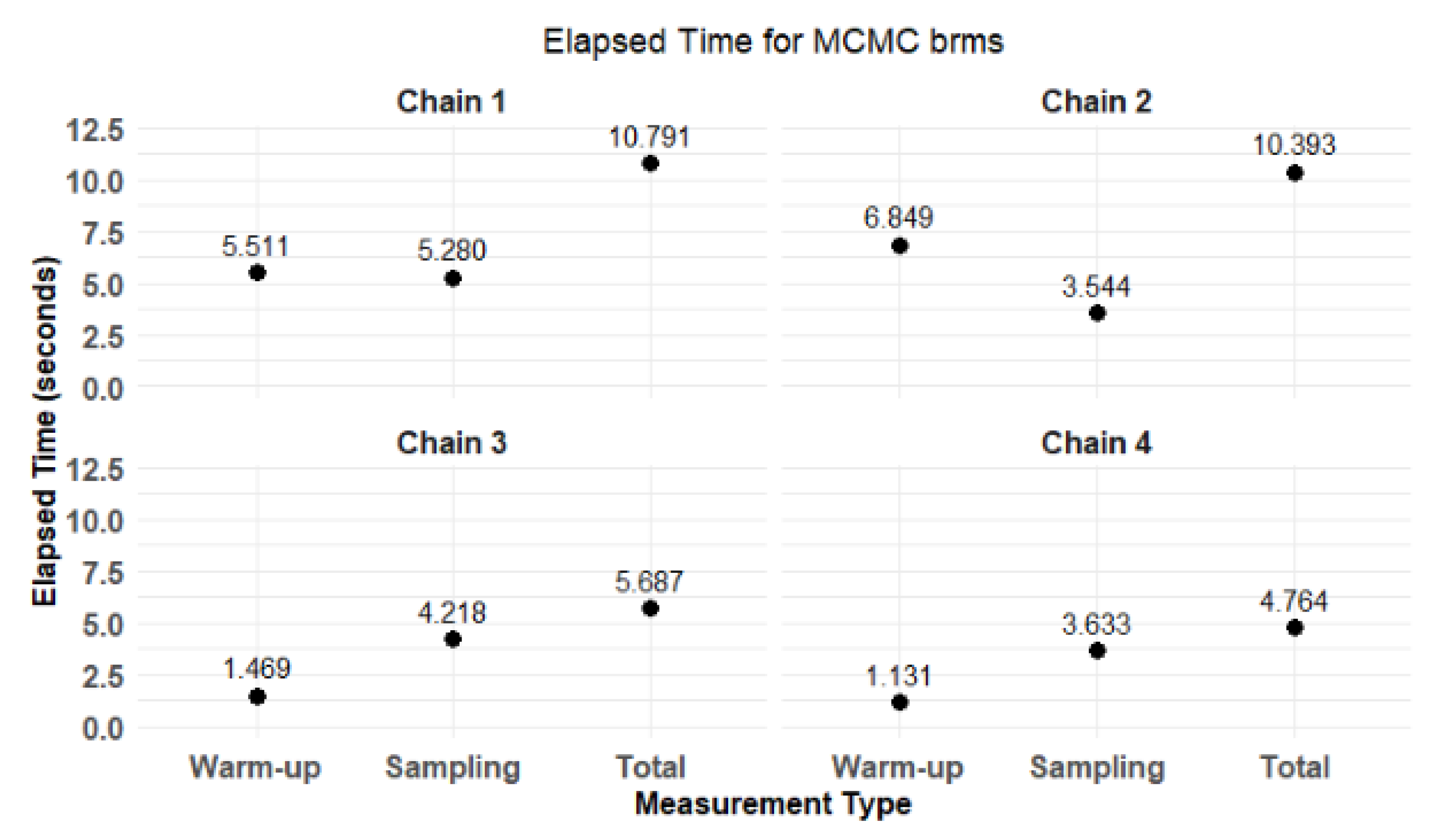
Figure 21.
AIC, BIC, and WAIC Values for Different Models.
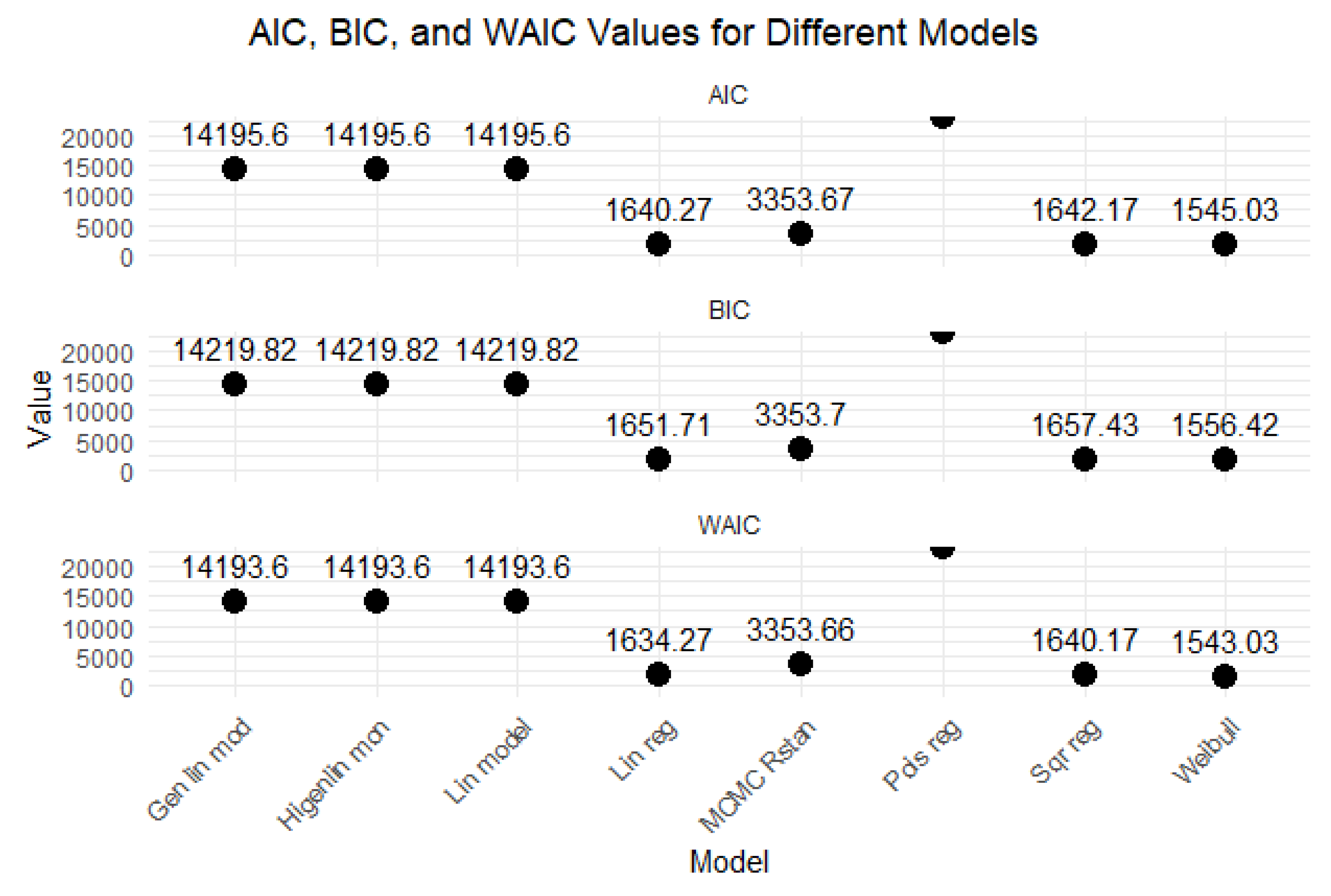

Table 1.
Photovoltaic panel failure causes and associated problems.
| Cause | Problem |
|---|---|
| Potential-Induced Degradation [9] | Ion migration and conductive paths |
| Aging and Environmental Factors [10] | Premature deterioration |
| Hot and Humid Climates [11] | Delamination and diode/box issues |
| Improper Tooling and Maintenance [12] | Damage to components |
| Light-Induced Degradation [13] | Loss of its rated wattage output |
| Bypass Diode Fault | Leakage current under temperatures |
Table 2.
Articles on photovoltaic panel modeling degradation.
| Method | Technique | References |
|---|---|---|
| Dynamic prediction | Hidden Markov Models | [26,27,28,29,30] |
| Statistical inference | Factor Analysis, Regression Analysis, MCMC with probabilistic programming | Factor Analysis [31,32,33,35], Regression Analysis [11,34,35], MCMC [36,37] |
| Machine Learning | Reinforcement learning, Deep Learning, Supervised learning, Cluster Analysis | Reinforcement learning [38,39,40,41], Deep Learning [8,42,43], Supervised learning [44,45], Cluster Analysis [46,47] |
Table 3.
Goals and formulas of used models.
| Model Type | Prediction Goal | Mathematical Formula |
|---|---|---|
| Linear Regression | Predicts continuous response variables (e.g., efficiency) based on predictors. | |
| Quadratic Regression | Captures non-linear relationships by including squared terms of predictors. | |
| Poisson Regression | Models count data related to degradation events (e.g., number of failures). | |
| Weibull Model | Analyzes time-to-event outcomes related to degradation (e.g., lifespan). | |
| Generalized Linear Model | Examines complex data structures with various response distributions. | |
| Hierarchical Linear Model | Accounts for nested data structures and variability among groups. |
Table 4.
Summary of AIC, BIC, and WAIC.
| Criterion | Basic Models | Linear Models | Advanced Models |
|---|---|---|---|
| AIC | 1545.032 (Weibull) to ∞ (Pois reg) | ∼14,195.6 | (MCMC RStan) |
| BIC | 1556.42 (Weibull), ∞ (Pois reg) | ∼14,219.82 | (MCMC RStan) |
| WAIC | 1543.032 (Weibull), ∞ (Pois reg) | ∼14,193.6 | – |
Table 5.
Performance metrics comparison.
| Comparison | Basic Models | Linear Models | Advanced Models |
|---|---|---|---|
| Basic vs. Linear Models | Basic models demonstrate significantly lower AIC, BIC, and WAIC values, indicating a better fit. | Linear models show high values across all criteria, suggesting they may not be suitable for the data. | The stark contrast in fit metrics suggests that basic models are preferable over linear models. |
| Basic vs. Advanced Models | Basic models outperform advanced models in AIC, BIC, and WAIC, with MCMC RStan showing extremely high values. | Advanced models, particularly MCMC RStan, do not provide a better fit than basic models. The high values for advanced models suggest they may not be necessary given the performance of basic models. | |
| Linear vs. Advanced Models | Linear models show high AIC, BIC, and WAIC values, similar to advanced models. | Advanced models do not significantly outperform linear models based on the provided metrics. The performance of both model types suggests that neither is particularly effective for the dataset. |
Disclaimer/Publisher’s Note: The statements, opinions and data contained in all publications are solely those of the individual author(s) and contributor(s) and not of MDPI and/or the editor(s). MDPI and/or the editor(s) disclaim responsibility for any injury to people or property resulting from any ideas, methods, instructions or products referred to in the content. |
© 2025 by the authors. Licensee MDPI, Basel, Switzerland. This article is an open access article distributed under the terms and conditions of the Creative Commons Attribution (CC BY) license (http://creativecommons.org/licenses/by/4.0/).
Copyright: This open access article is published under a Creative Commons CC BY 4.0 license, which permit the free download, distribution, and reuse, provided that the author and preprint are cited in any reuse.


