Submitted:
15 June 2023
Posted:
16 June 2023
You are already at the latest version
Abstract
For engines operating with heavy fuel oil (HFO), the nozzle rings of the turbocharger turbines are prone to severe degradation in terms of contamination with unburned fuel deposits. This contamination may lead to increased excitation of blade resonances. A previous study provides technical guidelines on how to extract the relevant information from the pulsation spectra by means of a single probe installed away from the turbine trailing edge and some sound experimental proofs of integral mode turbine vibration detection. These theoretical discussions only allude to the effects of mistuning and interferences due to classical blade passing frequencies on sound radiation patterns emitted by integral blade vibration modes. In this paper, both effects are thoroughly discussed. Combining the knowledge of theoretical study and further experimental results, the application range of this blade vibration detection method can be remarkably extended.
Keywords:
Turbocharger turbine blade vibration monitoring
; Pulsation measurement
; Nozzle ring fouling
; Mistuning
; Blade passing frequencies
Introduction
In a previous study (Ando, 2020), besides providing sound experimental evidence of turbocharger turbine integral mode detection by means of a pulsation sensor installed on the stator side away from the turbine trailing edge, theoretical backgrounds, mainly based on the work by (Mengle, 1990), were presented. During further investigations, however, it was recognized that the theories developed in the last 20 years of the 20th century, for example (Mengle, 1990) (Kurkov, 1981) and (Kurkov, 1984), handle mainly flutters of axial compressor stages and cannot apply directly to a turbocharger’s turbine integral mode resonances. Under a flutter condition, due to coupling between aerodynamic disturbance and structural eigenmode, IBPA (Inter-Blade Phase Angle) will tend to unify. Note that a spatial excitation force pattern covers the entire annulus, and it sweeps with a speed different from that of the rotor. Hence, the resulting resonance will become a non-integral mode. Therefore, theories at that time could have, at least provisionally, reasonably assumed a single IBPA over all blades.
On the other hand, in a turbocharger radial turbine stage, integral mode resonances are the main cause of an HCF (High Cyclic Fatigue) failure. As Figure 1 shows, especially during a low EO (Excitation Order) resonance crossing of a radial turbine stage, eigenfrequencies of the individual blades have a scatter magnitude up to a few percent.
In a low EO resonance, in contrast to NR (Nozzle Ring) vane count (>20) induced higher eigenmodes, the excitation force will not be distributed equally over the circumferences but tends to concentrate in a few angular positions, such as around the turbine casing tongue or a highly clogged NR sector. To simplify the following discussion, a single dominant excitation angular position is assumed, for example a completely clogged NR sector. With such an excitation force pattern, all low EO excitation force spatial phases will be locked to the position around the clogged NR sector. When the rotor sweeps through a resonance crossing, an individual blade reacts to the angularly fixed singular excitation force by alternating the vibratory phase from 0° (same phase as excitation) to +90° (resonance point) and +180° (“+” means, in this context, a lagging). Due to the mistuning, the vibratory phase alternation speed range differs between blades, so the IBPA will vary arbitrarily between zero and ±180° (“+” means, in this context, running in the same direction as the rotor revolution). From these considerations, at least in the case of a radial turbine stage’s low EO resonances, usage of the technical term “nodal diameter” is not appropriate, so discussion should be restricted only to IBPA. Additionally, the same “range” of IBPA will not cover the entire circumference but is confined to a few blade pairs. Note that it is a rather rare case that the IBPA will exactly fulfil the stepwise relation, , (: integer, a synonym of nodal diameter, and : Blade number).
The first topic of the present study deals, therefore, with adaptations of the theory developed by (Mengle, 1990) for a mistuned structure integral mode vibration with respect to the criterium of circumferential mode propagation in axial directions.
The second topic relates to interference between classical BPFs (Blade Passing Frequencies, pulsation peaks appearing at , with as blade count and as rotor revolution frequency, when blades are not vibrating) and the integral mode blade vibration-originating sound radiation. The low engine order fundamental mode resonance discussed in (Ando, 2020) or shown in Figure 1 occurs at around 70% of maximal rotor speed, at which the blade tip velocity is well below (M: Mach number). At a higher rotor speed, BPF airborne modes start to propagate undiminished in the axial direction, and pulsation amplitudes originating from BPFs will exceed by far those coming from a blade vibration, so that the detection of the blade vibration by means of a pulsation signal will become generally difficult. This study is intended to demonstrate how to handle and overcome the disadvantage of high revolution speed by analysing the experimental data in detail.
Theoretical discussions
The criterium for the propagation of circumferential mode in the axial direction
Prior to displaying the formula for axial wave number when blades are vibrating in a not negligible bulk flow rate as formulated in (Mengle, 1990), it is suggested first to review BPF mode axial direction propagation criteria postulated by (Tyler & Sofrin, 1962). Tyler & Sofrin formulated a simple criterium when the BPF mode, pure circumferential mode, will begin to propagate in an axial direction:
“In order that the pressure field of a spinning lobed pattern propagates in the duct (i.e., axial direction), the circumferential Mach number at which it sweeps the annulus walls must equal or exceed unity.”
In other words, if there are no bulk flow disturbances over the circumference, the BPF mode can propagate to the axial direction only when the blade tip velocity equals or exceeds the sound velocity. The so-called “Tyler & Sofrin mode,” i.e., due to interactions between a bladed rotor and stator, pressure fluctuation lobe numbers other than the rotor blade counts will arise, as discussed in the original paper, mainly in such a context that when the Tyler & Sofrin mode’s lobe number is less than the rotor blade counts, because the mode sweep velocity becomes higher than the blade tip velocity, even at a lower rotor revolution speed, the BPF noise will be audible from outside.
In principle, the simple criterium, i.e., circumferential mode sweep velocity ≥ sound velocity, should be applicable even when dealing with a blade vibration originating from a circumferential mode in a subsonic bulk flow rate. Now recall the axial wavenumber formula presented in (Mengle, 1990)
- Wave number in the axial direction
- : Axial bulk gas flow rate
- : Circumferential bulk gas flow rate (= blade tip velocity)
- : Speed of sound
- : Blade vibration frequency
- Wave number between blades in the circumferential direction, formulated as
- : Spacing between two blades
- : Integer varies between for an even number blades or for an odd number blades (synonym for nodal diameter)
- : Wave number between two blades (integer between )
- : Radius of blade tip
When the is set, provisionally, as zero, the blade vibration frequency can be expressed with by introducing a new term , the circumferential mode sweep velocity as defined in (Tyler & Sofrin, 1962) –:
By inserting equation (3) into (1), the criterion, whether a circumferential mode will propagate in the axial direction undiminished, i.e., the content of the root in (1) should be larger than zero, will become an easily comprehensible form:
At this stage, it is crucially important to notice that and relate not as scalar but as vector terms. That is, the sense “±” shall be added, which is missing in the formula in (Mengle, 1990). But, for example, (Zhao et al., 2015) put the “±” in the formula. Commonly, a frequency, i.e., oscillation cycles per time unit, is expressed as a scalar value since time has only positive values. If a point sound source is assumed, the sound will propagate in all directions, so that a , as a point source, cannot be defined as a vector. But, as a dominant circumferential mode arises through inter-blade interactions, it should be treated as a vector. The value of will be processed either as positive or negative, depending on the parameters in (2). So, there is no difference if “±” is explicitly put in (4). However, once this characteristic equation is expressed in the way it is in eq. (4), it becomes clear that the sense of circumferential mode sweeping direction relative to , the rotor revolution, takes a critical role for axial direction propagation characteristics. From these considerations, it can be presumed that airborne acoustic waves released from the suction (same direction as rotor revolution) or pressure (opposite direction to rotor revolution) side of a blade should have an entirely different axial direction propagation characteristic.
Integral mode blade vibration resonance frequency relates to rotor revolution frequency and EO, so that the sweep velocity can be formulated as:
At a given blade vibration resonance frequency, from eq. (5) it will be clear that the highest sweep speed in favour of axial direction propagation will result when the nominator takes the smallest positive value. Recalling that can take only values in the range for an even number of blades or for an odd number of blades, the highest positive value of is possible when (if takes a negative value) or when (if takes a positive value). This, by airborne acoustic conditions determined value, , will be commonly fulfilled in a radial turbine stage’s low EO resonances, which will be demonstrated theoretically and experimentally in later chapters.
The discussion takes into account the effect of mistuning. In the introduction, it is postulated that the integral relation between the IBPA and integer does not exist in a real structure and the IBPA will not have a single value in the whole blade counts. To make the point clear:
- : blade number, 1…
- : two-blade set varying inter-blade phase angle,
The main difference between (2) and (6) is that while in (2) each mode is assumed to stretch over the circumference, in (6) will be treated sector-wise. So, the commonly applied restriction, , will not be required anymore.
In a mistuned structure, while the value of is kept comparably the same for all blades, IBPA varies from sector to sector. In addition, referring to Figure 1, if one of the blades crosses a resonance point, a neighbouring blade does not vibrate significantly (see the response of blades 4 and 5 or 1, 2 and 3 in Figure 1). In an extreme situation, if only one blade is vibrating, then the IBPA will not be defined anymore. Conversely, an undefinable IBPA can be interpreted as a configuration that contains every possible IBPA value – like the Dirac Delta function that contains arbitrary frequencies. Refer to (Hanamura & Tanaka, 1980) for this basic idea.
The consequences of this theoretical consideration on blade vibration detection by means of pulsation sensors will be discussed in a later chapter by referring to experimental data and analysis.
Effect of subsonic bulk flow on airborne acoustic radiation amplitude and wave number
When dealing with the turbocharger’s turbine stage’s airborne acoustic field characteristics, it is indispensable to take the bulk flow into account because the Mach number of relative flow velocity exceeds 0.5. As displayed in Figure 2, in the case of the turbocharger’s turbine stage’s first flap mode, a higher magnitude of sound radiation will be released downstream than in the circumferential direction.
On the other hand, referring to (Morse & Ingard, 1986), amplitudes and frequencies of emitted sound at the upstream side will be amplified due to the bulk flow. The amplitude amplification magnitude at neighbouring blades’ trailing edges amounts to approximately four times when the bulk flow Mach number is 0.74 (see Figure 3).
The circumferential modes for those axial direction propagation characteristics discussed in the previous chapter shall establish themselves in the x-axis range -1 to 0 of Figure 3. So, the sound pressure amplitude, as well as wave number, are lifted two to five times compared to those without bulk flow. Interactions between neighbouring blades, enhancing or scattering depending on the IBPA, mainly occur at these elevated levels. Therefore, the from the blade originally emitted fraction directly to downstream will play a minor role, even if the fraction of original sound radiation has higher magnitudes.
Now returning to the statement about in the last chapter, that to favour an undiminished propagation in the axial direction, the should be zero, or most preferably +1 (when , mode sweep velocity will be “added” to , regardless of whether the IBPA has a positive or negative value). In the absence of bulk flow, at the first flap mode resonance condition along EO6, the wave number between two blades will amount to 0.38, i.e., the mode will be dominant. However, due to the bulk flow at the level of .74, as shown in Figure 3, the value will be amplified by two to three times, so that the actual wave number will lie between 0.76-1.14 in the range of blade row, i.e., the mode will be dominant.
Experimental Results and discussions
Concerning the experimental setup, refer to (Ando, 2020). A piezoresistive pulsation sensor was placed approximately 1.5 times the blade chord length away from the trailing edge on the downstream side. Eight optical sensors for BTT (Blade Tip Timing) were distributed near the blade trailing edge.
Figure 4 displays BTT measurements and a LSMF (Least Square Model Fit) analysis result as a nodal diameter trace, corresponding to the same resonance crossing as in Figure 1, refer to (Agilis measurement systems, 2022) for a description of the BTT data analysis method. Note that in BTT, LSMF analysis, because data sampling can occur only at discrete points of blade passing, FFT decomposition can also be conducted only at integer values in the range of =-5…+5 (for the blade count = 11).
Note also that the author is intentionally avoiding the wording of nodal diameter (“ND”) and uses the symbol “” (circumferential mode index). The notion of “nodal diameter” provokes an image that a wave pattern is distributed equally around circumferences. But as will be displayed later, in a mistuned structure, such an image represents by no means reality.
The highest amplitude is recorded in , not in . The rule about EO and excitable ND (EO=6, B=11) suggests that only ND =+5 must be excitable. This experimental result underlines that the notion of nodal diameter is inadequate for low EO resonances of a mistuned radial turbine.
Before presenting pulsation measurement results, let us recapture the frequency and wave number shift formulas in (Mengle, 1990) when the frame of observation is transformed from rotating to stationary, so that readers can follow further discussions easily.
- : circumferential mode index in rotating frame of reference
- : circumferential mode index in stational frame of reference
- : frequency in rotating frame of reference, i.e., blade vibration frequency
- : frequency in stational frame of reference
Recalling the previous discussion, that the = +1 mode will be dominant at the resonance condition of the 1st flap mode along EO6, depending on the circumferential mode index , a pulsation sensor detects the sound radiation at a different frequency or EO. If then EOpuls= 6-4+11=13. Consequently yields EOpuls=12, and to EOpuls=22, or 11 (coincides with BPFs).
Figure 5 c) displays the same trend, which is already presented in (Ando, 2020), but with additional information on individual blade trends. The pulsation amplitude trend along EO13, obtained by FFT and order tracking analysis, matches almost perfectly the BTT trace trend. Around the speed range where the amplitude peak arises, the blade vibration amplitudes of blades 5 and 6 or 7 and 8 were at comparable levels and the IBPA between the set of 5 and 6 or 7 and 8 met the prescribed value indeed for , i.e., 131°, refer to Figure 5 b). If the IBPA values lie within the given y-axis “range“ (115-147 degrees), the peak amplitude of FFT decomposition corresponds to the energy contribution of .
As demonstrated in Figure 5 c), the main peak of the BTT traces can be reconstructed only by the trends of blade pairs 5 and 6 and 7 and 8. The contributions of other blades are practically negligible.
Interestingly, around the main peak, IBPA values between 6 and 7 – refer to the blue cross symbol in Figure 5 b) – do not lie in the range. Instead, they are placed in the range for . In addition, especially at the resonance point of blades 5 and 6 – see the indication of ① in Figure 5 a) – the neighbouring blade 4 does not vibrate remarkably.
From the theoretical discussions in the previous chapters, it can be presumed that such sector-wise varying IBPAs or vibration amplitudes will influence sound radiation and interference characteristics in the downstream direction. To evaluate these presumptions, further investigations deploying computational fluid dynamics, as conducted by (Müller et al., 2018), would be desirable.
Figure 6 depicts the same kind of analysis as in Figure 5, but for the mode, proving that the blade vibration detection by means of pulsation sensor will also work well with another rather minor mode. Recorded pulsation peak amplitude along EO12 was approximately 1/3 of that in EO13. However, so far, the purpose of the method is condition-based monitoring and the monitoring will also work when pulsation signals along EO12 are tracked. Compared to the case with , the composition of contributing blades is more involved and will not be discussed further.
Finally, Figure 7 depicts the same kind of analysis as in Figure 5, but for the mode. Remember that the mode corresponds to the excitable circumferential mode along EO6 with blade count 11, and the observed EO, as a synonym for frequency from the stator side, will coincidence with the BPF and its harmonics.
In this case, due to interference with the BPF mode, the pulsation peaks originating from blade vibration go in the negative direction, but the trend itself represents well the mode as a “mirrored image.” The base level of the BPF increased roughly from 0.3 to 0.9 in the displayed speed range, while the negative peak amplitude due to blade vibration amounts to ca. 0.3-0.4. This finding – that the pulsation peak along EO = BPFs due to blade vibration can have a negative direction, and, as such, blade vibration can also be detected – opens further perspectives of application ranges for this method. The first flap mode resonance along EO6 discussed hereabove occurs around 70% of maximal revolution speed. Around maximal revolution speed, however, blade tip sweep speed becomes near to sound velocity, so that BPFs mode starts to propagate downstream undiminished.
Figure 7.
Comparison between BTT individual and traces with pulsation EO11 order tracking result (first flap mode along EO6).
Figure 7.
Comparison between BTT individual and traces with pulsation EO11 order tracking result (first flap mode along EO6).
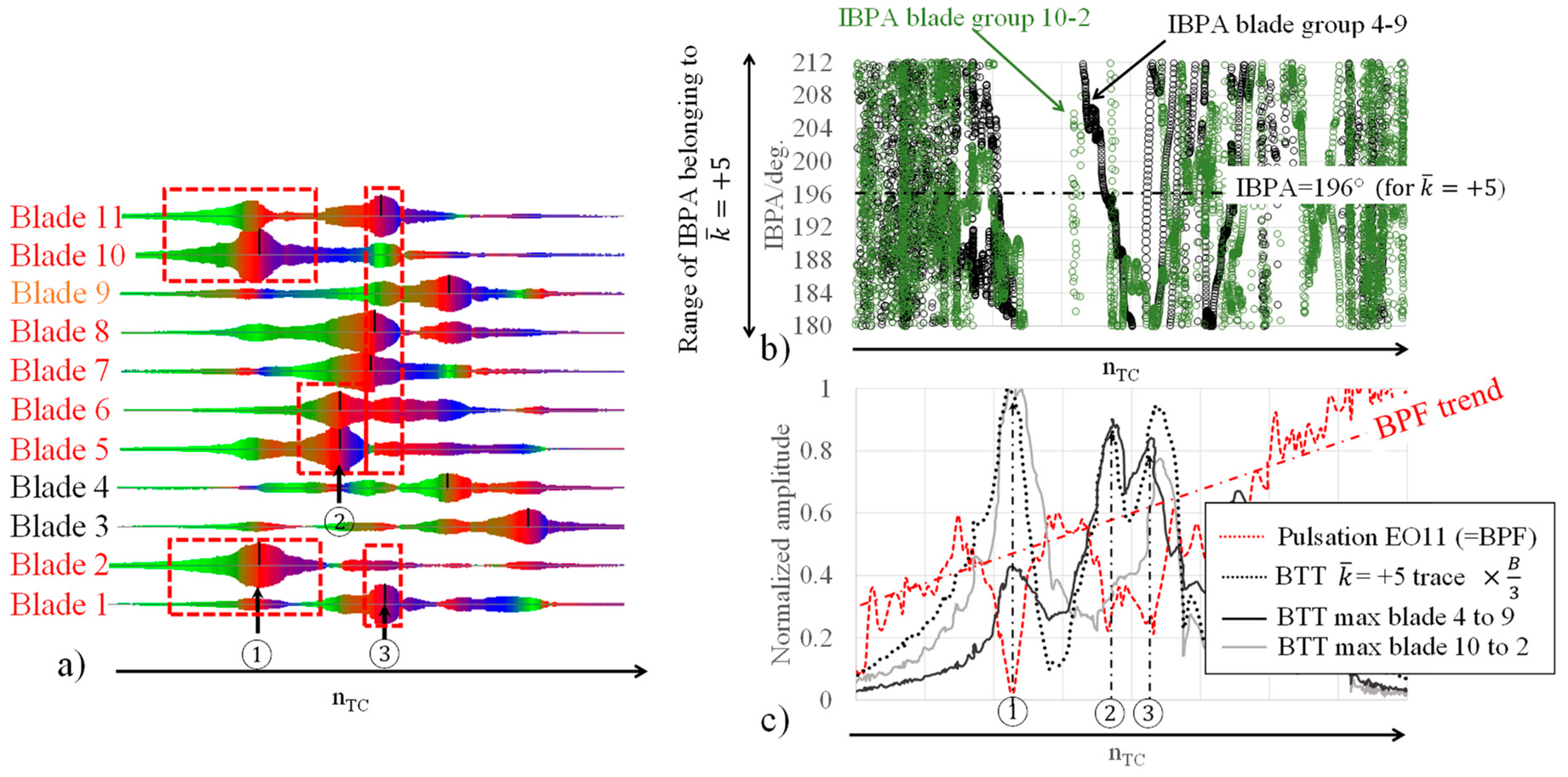
Figure 8 demonstrates that blade vibration detection will work with the method even when the blade tip speed is comparable to the speed of sound by analysing another 2nd mode resonance, which occurs along EO8. When the BPF mode starts to propagate undiminished, amplitudes will increase roughly fivefold, whereby the absolute pulsation amplitudes will exceed 100 mbar. The sharp drop of measured pulsation amplitude around the blade vibration resonance is, however, well distinguishable from gradual fluctuations originating from the BPF mode.
As demonstrated in Figure 8, by recognizing that pulsation peaks along BPFs can go in either a positive or negative direction relative to the base level, it can be claimed that this method can be applied for an entire (relevant) speed range to detect a potential danger of HCF failure.
Conclusions
In this study, it has been proven that integral mode blade vibration detection by means of a single pulsation probe located away from the trailing edge is possible even with an actual mistuned structure and that the application range can be extended up to the maximum turbocharger revolution speed, where the blade tip speed approaches the speed of sound. Even if airborne acoustic waves are radiated from just a few sectors of a bladed rotor, the pulsation sensor can sense them. In a real mistuned structure, each sector (such as a blade pair) can vibrate with an arbitral IBPA and the pulsation sensor on the stator side will sense these at different frequencies. By tracking several EOs neighbouring the BPF, circumferential mode distribution, i.e., mistuning of the structure, can also be estimated. For condition-based monitoring, the fingerprint of the structure, i.e., pulsation peak amplitude distribution along several EOs, can be used to crosscheck if an event may really be related to an HCF danger.
Another advantage of this method is that the pulsation amplitude does not depend on frame size, so once an alarm level is defined in a convenient frame size within the standard HCF qualification process, it will be applicable to other frame sizes.
 |
Nomenclature
| BPF | blade passing frequency |
| BTT | blade tip timing measurement |
| EO | excitation or engine order (low EO refers up to EO10, excitation originate from geometrical irregularities of casing and/or nozzle ring) |
| FFT | fast Fourier transformation |
| HCF | high cyclic fatigue |
| HFO | heavy fuel oil |
| IBPA | inter-blade phase angle |
| ND | nodal diameter (synonym for cyclic symmetrical mode) |
| LSMF | least square model fit used in BTT data analysis |
| NR | nozzle ring |
| B | turbine blade count |
| M | Mach number |
| U | axial bulk flow velocity |
| V | circumferential bulk flow velocity, = 2 · π · r · nrc |
| W | relative bulk flow velocity |
| co | sound velocity |
| cs | circumferential mode sweep velocity |
| i | natural number |
| k | integer in the range of for odd number blade count |
| circumferential mode index | |
| m | airborne acoustic wave number between two blades |
| nTC | rotor revolution frequency |
| r | outer radius at blade trailing edge |
| ω | blade vibration frequency |
| axial wave number defined by equation (1) | |
| global wave number between two blades defined by equation (2) |
References
- Agilis Measurement Systems. 2022. Available online: https://agilismeasurementsystems.com/.
- Ando, T. 2020. Pulsation and Vibration Measurement on Stator Side for Turbocharger Blade Vibration Monitoring. Int. J. Turbomach. Propuls. Power 5: 11. [Google Scholar] [CrossRef]
- Hanamura, Y., and H. Tanaka. 1980. A simplified Method to Measure Unsteady Forces Acting on the Vibrating Blades in Cascade. Bulletin of the JSME 23: 880–887. [Google Scholar] [CrossRef]
- Kurkov, A.P. 1981. Flutter Spectral Measurements Using Stationary Pressure Transducers. J. Eng. Power. 103: 461–467. [Google Scholar] [CrossRef]
- Kurkov, A.P. March 1984. Formulation of Blade Flutter Spectral Analyses in Stationary Reference Frame. Washington, DC, USA: NASA TP-2296; NASA. [Google Scholar]
- Mengle, V.G. Acoustic spectra and detection of vibrating rotor blades including row-to-row interference. Proceedings of the AIAA 13th Aeroacoustics Conference, Tallahassee, FL, USA, 22–24 October 1990. [Google Scholar]
- Morse, P.M., and K.U. Ingard. 1980. Theoretical Acoustics. Chapter 11. ISBN 0-691-02401-4. [Google Scholar]
- Müller, T.R., and et al. 2018. Influence of Interflow Interaction on the Aerodynamic Damping of an Axial Turbine Stage. Proceedings of the ASME Turbo Expo 2018, GT2018-76777. [Google Scholar]
- Tyler, J.M., and T.G. Sofrin. 1962. Axial Flow Compressor Noise Studies. SAE Transactions 70: 309–332. [Google Scholar]
- Zhao, F., and et al. Influence of Acoustic Reflection on Flutter Stability of an Embedded Blade Row. Proceedings of the ETC11, 23–27 March 2015. [Google Scholar]
Figure 1.
Response of blades at a first flap mode along excitation order six (for a radial turbine).
Figure 1.
Response of blades at a first flap mode along excitation order six (for a radial turbine).
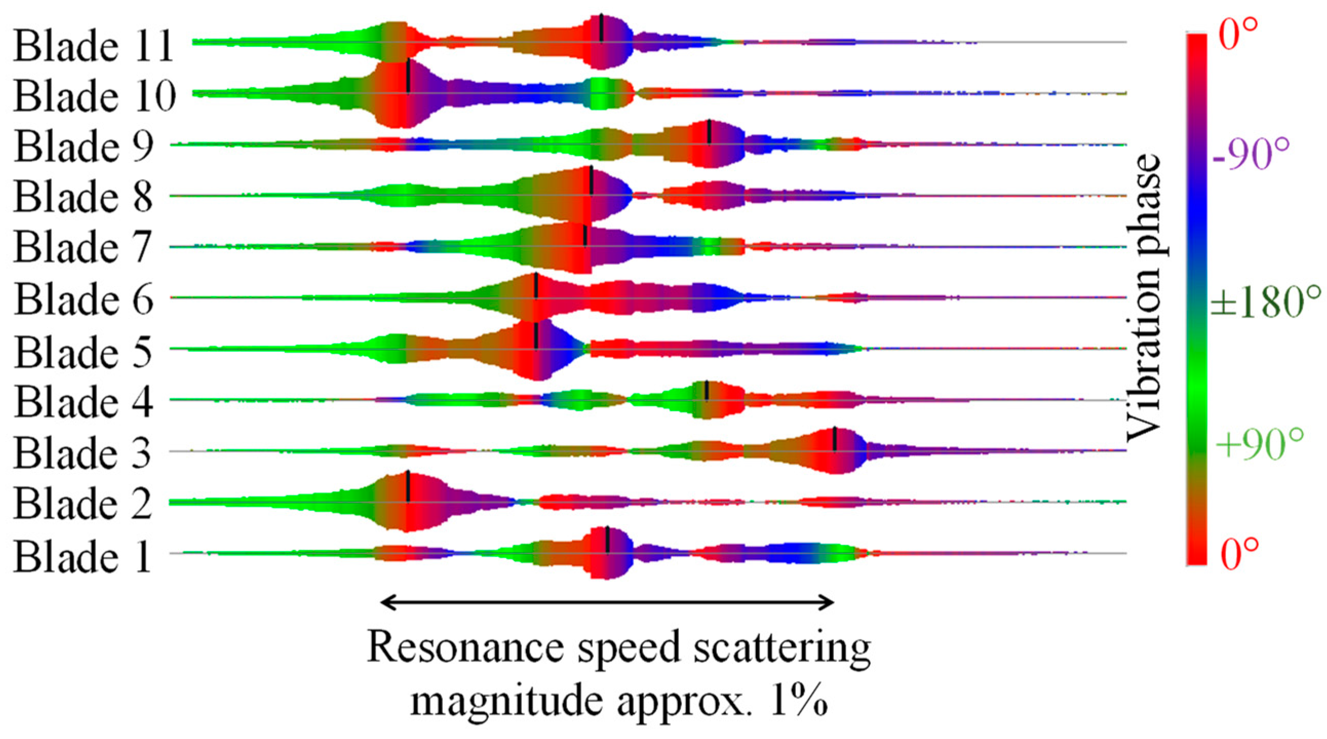
Figure 2.
First flap mode shape and geometrical relation (left picture displays ND4 mode).
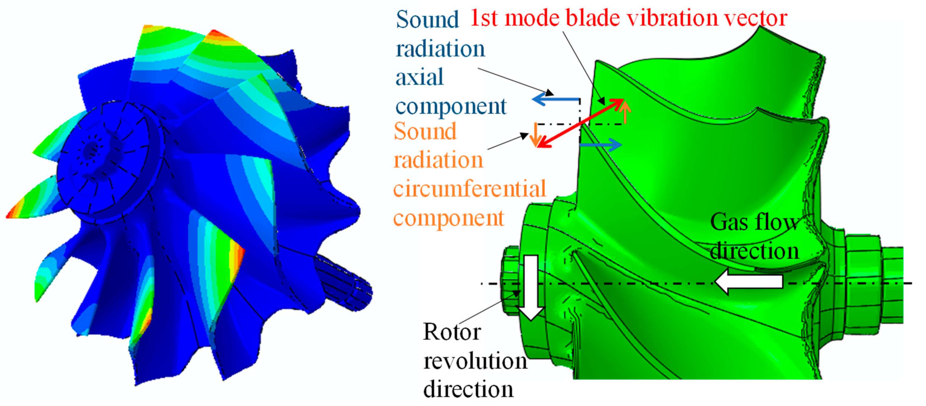
Figure 3.
Emitted sound amplitude amplification behaviour due to bulk flow with M=0.74 (first flap mode).
Figure 3.
Emitted sound amplitude amplification behaviour due to bulk flow with M=0.74 (first flap mode).
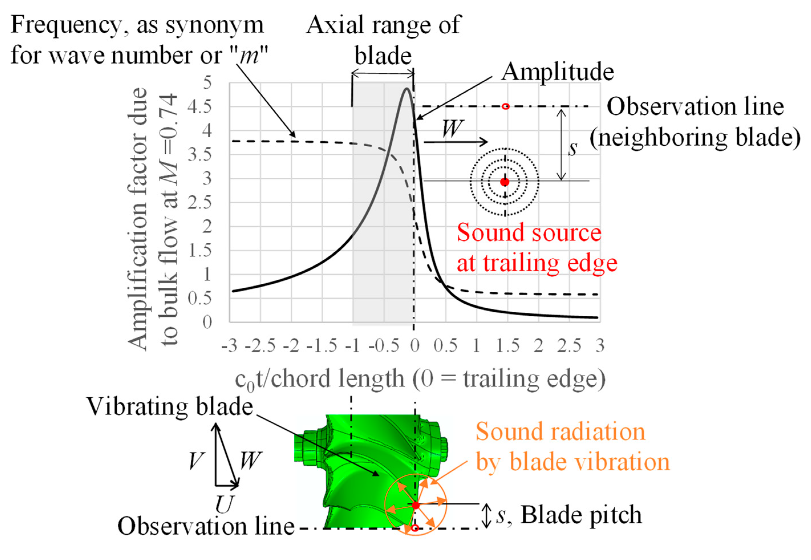
Figure 4.
BTT nodal diameter trace output, normalized by the highest amplitude, resulted in =-4 (in the diagram, trend of all values -5…+5 is included but highlighted only values used for further discussion).
Figure 4.
BTT nodal diameter trace output, normalized by the highest amplitude, resulted in =-4 (in the diagram, trend of all values -5…+5 is included but highlighted only values used for further discussion).
Figure 5.
Comparison between BTT individual and traces with pulsation EO13 order tracking result focusing on the behaviour of blades 4-9 (first flap mode along EO6).
Figure 5.
Comparison between BTT individual and traces with pulsation EO13 order tracking result focusing on the behaviour of blades 4-9 (first flap mode along EO6).
Figure 6.
Comparison between BTT individual and traces with pulsation EO12 order tracking result (first flap mode along EO6).
Figure 6.
Comparison between BTT individual and traces with pulsation EO12 order tracking result (first flap mode along EO6).
Figure 8.
Comparison between BTT traces with pulsation EO11 order tracking result for a 2nd blade eigenmode resonance along EO8 occurring at around max. nTC.
Figure 8.
Comparison between BTT traces with pulsation EO11 order tracking result for a 2nd blade eigenmode resonance along EO8 occurring at around max. nTC.
Disclaimer/Publisher’s Note: The statements, opinions and data contained in all publications are solely those of the individual author(s) and contributor(s) and not of MDPI and/or the editor(s). MDPI and/or the editor(s) disclaim responsibility for any injury to people or property resulting from any ideas, methods, instructions or products referred to in the content. |
© 2023 by the authors. Licensee MDPI, Basel, Switzerland. This article is an open access article distributed under the terms and conditions of the Creative Commons Attribution (CC BY) license (http://creativecommons.org/licenses/by/4.0/).
Copyright: This open access article is published under a Creative Commons CC BY 4.0 license, which permit the free download, distribution, and reuse, provided that the author and preprint are cited in any reuse.


