Submitted:
27 May 2023
Posted:
30 May 2023
You are already at the latest version
Abstract
Lubricated tribosystems such as main-shaft bearings in gas turbines have been successfully diagnosed by oil sampling for many years. In practice, the interpretation of wear debris analysis results can pose a challenge due to the intricate structure of power transmission systems and the varying degrees of sensitivity among test methods. In this work, oil samples acquired from the fleet of M601T turboprop engines were tested with optical emission spectrometry. Two-way analysis of variance (ANOVA) with interaction analysis and post hoc tests were carried out on measurement data from the whole fleet of the M-601T turboprop engines to study the impact of aluminum and zinc concentration on iron concentration. Finally, the developed model was used to evaluate the oil testing results for two specific engines of this type. Thanks to ANOVA, the assessment of engine health is based on a statistically proven correlation between the values of the dependent variable and the classifying factors.
Keywords:
wear debris
; oil analysis
; emission spectroscopy
; turboprop
; propeller governor
; ANOVA
; interaction analysis
; condition indicator
1. Introduction
Oil debris monitoring aims to detect wear particles whose characteristics and numbers differ from those generated during normal operation of the tribological system. It has been successfully used for the health assessment of tribological systems for several decades [1,2,3]. There are many examples when bearing, transmission or hydraulic system failures were detected in time. The development of specialized spectrometers [4] made it possible to measure element concentrations with growing precision and process them statistically to set alarm thresholds. However, no oil testing method is universal, and thus various analytic techniques are usually used side by side. In a traditional offline approach, oil samples are taken from the engine at regular intervals and sent to a laboratory for analysis. Recently, online oil debris monitoring [5,6,7] has become more and more common. It involves installing magnetic [8,9,10], capacitive [11,12], optical [13,14,15] or acoustic sensors [16] in the engine. These sensors can count particles or measure their diameters but most of them are unable to identify material or detect fine wear debris. Therefore, used oil is still laboratory tested despite the considerable workload and cost related to taking, shipping and testing samples.
The measured concentrations of elements and other oil parameters are processed statistically to establish alarm thresholds. The traditional approach is based on the normal distribution, and assumes triple standard deviation (3) to be the warning limit (yellow) and 4 to be the alarm level (red). If the distribution is not normal, the cumulative distribution is alternatively used to set the warning and alarm limits [17]. In the common data interpretation procedure, level and trend status data from individual test methods are fused to evaluate an overall risk of failure and make maintenance decisions [18,19]. The failure mode matrices are used to link the various concentration level and trend statuses with the specific condition indicator (Normal, Alert, Urgent, Hazard, Danger) and potential cause.
Pair-wise analytical techniques such as correlation [20,21,22] or regression are widespread in oil analysis because relying on a single parameter may not provide reliable solutions, and may also overlook significant diagnostic information. Correlation describes a statistical relationship between two random variables. When both variables follow a normal distribution, the Pearson correlation coefficient is used. Otherwise, the Spearman correlation should be employed since it is more general and robust to outliers [23,24]. Other multivariate statistics such as cluster analysis, principal component analysis or factor analysis are common as well.
According to the review by Wakiru et al. [25], statistical methods account for 31% of publications on oil analysis, artificial-intelligence (AI) approaches for 37%, model-based for 13%, and hybrid for 19%. Even if AI is the main tool, statistical methods are useful to understand the data, select features and validate the results. For example, Rodrigues et al. used Artificial Neural Networks (ANN) and Principal Component Analysis to classify the oil condition in a fleet of bus diesel engines [26]. Gajewski and Valis proposed multilayer perceptron and radial basis function neural networks to evaluate oil samples from diesel engines of heavy crawlers [27]. Zhao et al. fused vibration based-features with relative kurtosis and skewness of the ferrous particle size distribution to feed three machine learning classifiers i.e. support vector machines (SVM), k-nearest neighbors, and decision tree [28].
The presented efforts are focused on finding relations and patterns in oil testing results, essential for supporting maintenance decisions in gas turbines, helicopters, diesel engines and wind turbines. However, the interpretation of oil analysis results still poses a challenge when the trends are erratic or individual evaluation methods provide contradictory indications. More efficient oil analysis methods are still being sought to ensure the reliable and safe operation of aircraft engines.
In this work, analysis of variance is used to model the impact of aluminum and zinc concentration on iron concentration. These elements make up materials used in the rotating and stationary engine components i.e. steel and aluminum alloys. It will be shown that the number of iron particles produced in friction pairs is correlated to aluminum and zinc production. This correlation will provide a basis to set alarm thresholds and detect accelerated wear.
2. Materials and Methods
2.1. M601T Turboprop
Walter M601 was developed in the early 1970s for the L-410 Turbolet aircraft as an alternative to the PT6 turboprop [29,30]. The engine variant M601T, designed later for aerobatic applications, required some design changes, such as the reinforced drive shaft and compressor casing, modified lubrication system and others. The engine was produced by Walter Aircraft Engines (now GE Aviation Czech s.r.o.) for the Polish PZL company to power its PZL-130 Orlik TC-I trainer. Its nominal power was 490 kW.
The M601T turboprop pulls the aircraft, so its internal flow is reversed and the air intake is located in its rear part while there are two elbow exhaust outlets in the front [31,32]. The turboprop consists of two basic sections - a gas generator and a drive unit (Figure 1). The gas generator includes an inlet and a combined compressor – two axial and one centrifugal stage with a total compression of 6.55, an annular combustor, a single-stage generator turbine, an accessory gear box with a fuel control unit and an electric starter. The drive part of the engine consists of a power (free) single-stage turbine, a two-stage, pseudoplanetary reduction unit and exhaust outlets. The reduction unit drives the propeller and its governor, and it also supplies the propeller unit with pressurized oil.
The engine oil system includes gear pumps and an integrated oil tank with a capacity of 7 liters, and a minimum oil level of 5.5 liters. The overall amount of oil in the system is 11 liters. The nominal oil consumption is 0.1 liters per hour [31].
The time between overhaul (TBO) of M601T operated at PZL-130 Orlik was only 500 flight hours (FH). In service, the propeller governor (LUN 7816) turned out to be the weakest part of the M601T engine and, in the 1990s and early 2000s, its accelerated wear contributed to some air accidents and incidents of the trainer [33]. Consequently, LUN 7816 had to be serviced every 140 FH by the manufacturer. Oil testing and vibration measurement were carried out for engine health monitoring [34,35]. A magnetic plug in the reduction unit was a primary tool to detect oil debris. Additionally, oil was sampled every 10 FH from the tank, reduction unit and AGB and tested in an accredited laboratory [36]. Samples were taken after the flight, at the appointed time after engine shutdown to ensure sample homogeneity and eliminate the error caused by the sedimentation of wear products. The applied methodology followed the JOAP procedures [37].
2.2. Atomic Emission Spectrometry
Spectrometric oil analysis is a diagnostic maintenance tool used to determine the type and amount of wear metals in lubricating fluid samples [37,38,39]. In rotating disc electrode atomic emission spectroscopy (RDE-AES), the wear products contained in the tested oil are excited by an electric arc between graphite electrodes, and the obtained spectral lines are analyzed. The emitted radiation, after splitting on a prism, falls on a plate that transmits radiation with the wavelengths characteristic of the chemical elements under study [40,41]. The measurement is performed on the emission spectrometer simultaneously for several metallic elements. Concentration is measured in parts per million (ppm) i.e. milligrams per kilogram.
The used spectrometer was SpectrOil M by AMETEK Spectro Scientific [42]. It consists of three main components: excitation source, optical system and readout system. It has the range of 0-1000 mg/kg for iron, aluminum and zinc. The measurement uncertainty is 10%. Data evaluation criteria and corresponding concentration limits are defined for several military engines by Volume III of the US Joint Oil Analysis Program (JOAP) manual [43]. For M601T and other engines not covered by the standard, alarm thresholds have to be set individually.
The application of RDE-AES in oil analysis is limited by particle size [44,45,46]. It is assumed that it is effective in analyzing debris no greater than 8-10 µm. Therefore, the indication of abnormal wear by spectrometry should be verified by alternative analytic methods e.g. ferrography.
There are well-known guidelines for the analysis of spectrometry results [37,47,48]. Detected metal debris can be divided into wear products, oil contaminants or additives. Certain metallic elements can provide clues concerning the parts being worn, but others only offer a general indication of accelerated degradation. Sometimes even the slightest increase or presence of a specific element can be cause for alarm.
In the engine, there are many sources of particles containing iron and aluminum because they are present in many components. Aluminum is mainly a wear product but it can also come from the environment with silicon as dirt contamination. Iron is the most common metal, so its concentration is higher than other elements even without excessive degradation [49]. The concentration of wear metals slowly grows at a constant rate during normal operation. Zinc is used with copper in brass fittings and galvanized surfaces. Regrettably, the origin of the wear could not be determined for the M601T engine since information about the materials was scarce.
2.3. Analysis of Variance
The Analysis of Variance (ANOVA) method, initiated by Fisher in the 1920s, is a statistical tool to analyze the differences among means [50]. It assesses the impact of the independent classifying factor (j=1....,m) on the distribution of the dependent (explained) variable y. The levels of the classifying factor (groups) can be binned values or categories. The method analyzes the significance of differences between the means calculated from observations coming from individual groups. The following assumptions of ANOVA have to be met:
- Distribution of the dependent variable is normal for each group,
- Variance between groups is similar.
ANOVA is resistant to minor deviations from the normality of the distributions and to small differences in variances between individual groups. To verify the assumption about the normal distribution of the dependent variable, the following statistical tests were used: Shapiro-Wilk, Jarque-Bera and Lilliefors. To verify the assumption about the homogeneity of variance, Bartlett’s, Levene’s or Cochran’s tests were used.
There are numerous applications of ANOVA in various disciplines, including wear or oil condition analysis. Holland et al. applied Fourier transform infrared (FT-IR) spectroscopy and ANOVA to assess water contamination in oil [51,52]. Liu et al. used optical measurement to monitor oil debris and viscosity while ANOVA was utilized to assess the significance of the model equation [53]. Cetin et al. studied the concentration rate and aggregation behavior of nano-silver added colloidal suspensions on the wear behavior of metallic materials [54]. Tian et al. investigated the degeneration of synovial joints and used ANOVA to evaluate the significance of 32 wear parameters obtained by 3D optical surface characterization [55]. Mason et al. evaluated the bearing spall propagation results with ANOVA [56]. Woma analyzed the wear performance of vegetable oils used as lubricants [57]. Azcarate et al. evaluated D-optimal mixture designs for microwave-induced plasma optical emission spectrometer. ANOVA is also frequently used to analyze metal contaminants in food, drugs or water with atomic emission spectrometry. However, we could not find any publications in which ANOVA was employed in oil analysis for modeling wear metal concentration.
This study aims to determine whether the concentrations of aluminum and zinc affect the concentration of iron. Therefore, the concentrations of aluminum and zinc are classifying factors, while the dependent (explained) variable is iron concentration.
The following tasks were performed to implement ANOVA for wear debris analysis:
- Conduct Exploratory Data Analysis to study concentration distributions and understand the data.
- Run tests for the homogeneity of variance to select the best variant of binning aluminum and zinc data into concentration levels.
- Bin the data into four Al and Zn levels and remove outliers.
- Transform iron concentration to normal distribution.
- Tests the normality of transformed iron distributions in individual groups.
- Calculate two-way ANOVA.
- Run post hoc tests.
- Analyze Interaction Plots.
- Use the model to set the individual limits of iron concentration for each factor level.
- Compare the sample testing results with the defined limits to make a maintenance decision.
3. Results
3.1. Dataset
The oil samples acquired from the fleet of 29 M601T engines operated over five years were tested using optical emission spectrometry with a rotating electrode. The dataset included 1250 samples with the measured concentrations of 19 elements: Ag, Al, B, Ba, Ca, Cr, Cu, Fe, Mg, Mo, Na, Ni, P, Pb, Si, Sn, Ti, V and Zn. The elements whose concentration exceeded the threshold of 1 ppm were selected for statistical analysis. In this case, only aluminum, iron and zinc met this condition while other elements generally produced negligible values. The observed iron concentrations were the highest because this element is contained in many alloys used in the engine. For this reason, iron was selected as a dependent variable and its values were used to classify engine health.
The following plots present the distribution of iron (Figure 2), aluminum and zinc (Figure 3). Iron distribution is close to normal but has a positive skew of 1.68. Scatter plots (Figure 4) confirm that there is some positive correlation between elements, higher for aluminum than for zinc. The Pearson correlation coefficients are presented in Table 1.
3.2. Binning Al and Zn Concentrations
To perform ANOVA, Al and Zn concentrations have to be binned into some groups. Therefore, the range of their observations was divided into a number of equal bins, with the right endpoint chosen to include 99.7% of observations (three-sigma rule). Several binning variants were tested for ANOVA’s assumptions to be met. Therefore, Bartlett’s and Levene’s tests were used to evaluate iron variance homogeneity between individual Al and Zn levels. Outliers (with values greater than Q3 + 1.5 IRQ) were removed before the tests.
Table 2 presents the probability values produced by Bartlett’s and Levene’s tests for the increasing number of aluminum and zinc levels. Probabilities exceeding 0.5 are marked in green. The case of two Al and Zn levels was analyzed further, but it was found that iron concentration in some of these groups did not pass distribution normality tests (Lilliefors, Jarque-Bera or , Table 3) and consequently, ANOVA could not be performed.
3.3. Transforming Data to Normal Distribution
Since iron concentration did not meet ANOVA assumptions in any tested binning variant, data transformation was applied using the natural logarithm function:
A similar testing procedure was carried out for the transformed data to check the homogeneity of variances between groups and find the best binning variant. The value of parameter b was sought iteratively (Figure 5).
Table 4 shows the estimated probability values of Bartlett’s and Levene’s tests for different numbers of classification factors (ranges of aluminum and zinc concentrations) after the logarithmic transformation of the data. The table shows the value of factor b, for which the highest probability values for both aluminum and zinc levels were obtained. Green indicates the probability that exceeds the limit of 0.5. The case of four groups and parameter b=9 achieved the highest probability both for aluminum and zinc, so it was selected for further analysis of variance.
The aluminum and zinc concentration levels chosen for binning into four groups are specified in Table 5. The corresponding iron distributions are presented in Figure 6. These box plots show some outliers (with values greater than Q3 + 1.5 IRQ), which were removed from each group before further analysis. Then, the group means and standard deviations (Std) of transformed iron concentration were calculated (Table 5).
Then, the distributions of transformed iron for four levels of aluminum and zinc concentration were tested for normality (Table 6. At least one of three tests suggested accepting the null hypothesis in each case, so the distributions could be considered normal and the assumptions of ANOVA were satisfied (at the 5% significance level).
3.4. Two-Way ANOVA
A two-factor analysis of the variance of transformed iron was performed for four levels of aluminum and zinc concentration. The ANOVA table (Table 7) shows the effect of these factors on iron concentration, without testing interactions.
In both cases, comparing the determined values of F (165.42 and 9.91) with its critical values, we decide to reject the null hypothesis about the equality of means in all groups in favor of the alternative hypothesis that there is an impact of both aluminum and zinc on iron.
There is a significant difference in the sum of the squares between aluminum (1.063) and zinc (0.056). This indicates that aluminum has a greater impact on iron concentration (27.9%) than zinc (1.5%). This can be confirmed by comparing the mean values of the different groups of aluminum and zinc. The means of aluminum groups varies more from each other than zinc groups (Table 5).
The attempt to perform ANOVA with testing interaction effects failed due to incomplete data representation, i.e. there were no observations belonging to the paired groups Al 1 Zn 3 and Al 1 Zn 4. This is illustrated by a grouped boxplot in Figure 7. The issue was solved by removing the data from group Al 1 and then ANOVA with interactions was smoothly completed (Table 8). Removing Al 1 did not affect the diagnostic reasoning, since it contained only 85 data points with the lowest concentration.
Based on the F test result (Prob>F), the null hypothesis that there are no differences between means in individual groups should be rejected. The table shows that both the concentration of aluminum and zinc, but also interaction between these concentrations affect the results of iron. Effect size shows that the greatest impact has aluminum concentration (22.7%), then zinc concentration (2.1%) and the least interaction between aluminum and zinc (0.5%).
3.5. Post Hoc Tests
After receiving ANOVA results confirming statistically significant differences between the means of individual groups, the next step is to perform post hoc tests. Since ANOVA verified only that means in some groups are not equal, these tests are necessary to determine which groups’ means are significantly different. There are several post hoc tests which use different approaches and some of them are considered conservative. In this work, the least significant differences test (LSD), Bonferroni’s, Scheffé’s and Tukey’s tests were used.
The results of post hoc tests for aluminum concentration levels are presented in Table 9 and Table 10. All the performed tests confirmed that the means in all groups significantly differ from each other at the 95% confidence level. Their confidence intervals did not include zero for any pair of means analyzed.
The results of LSD, Bonferroni’s, Scheffé’s, Tukey’s tests for zinc concentration levels are presented in Table 11 and Table 12. All the post hoc tests showed that the mean values for Zn concentration levels are significantly different at the 95% confidence level, except the Zn 3 and Zn 4 groups. Since the confidence interval of this pair of levels includes zero (marked in yellow), it can be concluded that the averages of these groups do not differ significantly. This is also confirmed by Figure 6 where overlapping of Zn 3 and Zn 4 intervals is visible.
For all the performed tests, zinc compared to aluminum was characterized by the lower absolute values of differences of group means, which is in line with the effect sizes calculated by ANOVA.
3.6. Interaction Effects
Interaction plots are a convenient way to illustrate how factors influence iron concentration and further analyze their interactions. These plots have the group means of the dependent variable on the ordinate and the level of one of the factors on the abscissa. The levels of the second factor correspond to individual data series in the plot. The shape of the polylines – their crossing, curving and parallelism – inform about the effects of interaction.
Figure 8a shows iron as a function of aluminum levels 2-4. The lines are almost parallel with a deviation at Al 3 for Zn 4 line. Small distances between the lines indicate that there is a small effect of zinc while the high slope of the curves confirms a clear effect of aluminum.
Similarly, Figure 8b with iron versus Zn levels shows roughly parallel lines with deviations at Zn 4 for Al 3 line. The low slope of the curves confirms that there is a small effect of zinc while considerable distances between the lines indicate a clear effect from aluminum. The disturbance from parallelism at two points suggests the existence of interaction, i.e. at different levels of aluminum concentration, zinc concentration affects the concentration of iron differently. Interaction plots are in line with effect sizes produced by ANOVA (Table 8), which suggested a significantly higher impact of aluminum than zinc or their interactions.
3.7. Setting Condition Indicators
Based on the presented ANOVA results, it can be assumed that for the average M601T engine, during normal operation, iron concentration for individual aluminum and zinc levels should remain within limits defined by the statistical model (Table 13). These limits corresponded to two-sigma intervals in these groups.
3.8. Engine 1
The obtained ANOVA model was used to evaluate the wear of two engines.
For engine 1, oil samples were collected from the tank every 10±2 FH between it accumulated 697.6 and 1254 FH (in total 57 samples). The scatter plot (Figure 9) presents the iron results as a function of the aluminum or zinc concentration along with the boundaries of their four levels and the corresponding iron limits. The measurement uncertainty of 10% must be taken into account when classifying the results.
It is noticeable that one iron data point exceeded the upper limit of iron concentration at AL 3. In contrast, as a function of zinc concentration, four iron concentration values exceeded the upper limit of iron concentration at ZN 1.
Figure 10 shows the time series of iron, aluminum and zinc concentration along with their level number. The moments when the upper limit of iron concentration was exceeded are marked with a cross mark symbol. When iron concentration exceeded the Al-related limit, the zinc-related limit was also exceeded. Three other Zn 1 exceedances are located nearby.
From the maintenance records of the aircraft, it was found that the oil sample taken at 753.33 FH was the first sample taken after the overhaul. In addition, after sampling the oil at 780.9 FH, the oil was changed. Before the overhaul, the upper limit of iron concentration value had not been exceeded. Therefore, the above results indicate that the contamination of the lubrication system after the overhaul distorted the statistically proven correlation between the discussed elements. After the oil change, no further deviations from the calculated correlation were found during the next 450 FH.
3.9. Engine 2
Engine 2 accumulated 808.08 FH when the first oil sample was taken. Before reaching 1114.38 FH, the 33 oil samples were collected and analyzed. Figure 11 shows the obtained iron results as a function of aluminum or zinc concentration. The plots show that iron concentration exceeded the upper limit for some aluminum and zinc levels.
Figure 12 shows the time series of iron, aluminum and zinc concentration with their level number. The moments when the upper limit of iron concentration was exceeded are marked with a cross mark symbol. In the first 80 FH, iron concentration did not cross the limit but later numerous exceedances were observed. Several oil changes combined with the flushing of the system led to a temporary reduction in particle concentration and getting some observations that were within the limits. However, these actions did not reverse the overall trend of growing iron production.
The traditional analytic approach (3) classified the observed iron results 5.5-7.5 ppm as acceptable in the four-point scale: 1) white - undamaged or new, 2) green - acceptable wear, 3) yellow - increased wear, 4) red - significant deterioration. It can be concluded that although iron concentration was only at the yellow level, the ANOVA-based model indicated accelerated wear of the system. Already 215 FH before detecting unacceptable particles at the magnetic chip detector, symptoms of damage appeared in the form of a distorted correlation between the concentration of the discussed elements. Even repeated oil changes and other maintenance actions such as replacing the propeller governor did not result in a permanent return to the correct correlation of results.
The process of accelerated wear distorted the statistical dependence between the elements because it triggered the generation of particles in larger quantities and with an unusual distribution. Since iron concentration persistently exceeded the limits for some Al an Zn levels, the engine was subjected to supervised maintenance which involved more frequent check-ups. This procedure made it possible to continue engine operation safely and avoid the costs of a premature overhaul. However, upon reaching 1114 FH, hairy chips up to 3 cm long were found on the filter of the propeller reduction unit along with numerous metallic particles on the magnetic plug of AGB (Figure 13). The engine was grounded and sent to the repair shop.
4. Discussion
ANOVA was employed here to prove the statistical dependence between iron and aluminum or zinc, and to calculate the effect size for each factor. Its results led us to rejecting the null hypothesis of mean equality in individual groups. This confirms that with the increase in the concentration of aluminum and zinc, higher average values of iron concentration are obtained (except Zn 4 level). Therefore, their concentrations should be analyzed jointly in this tribological system (the M601T turboprop) since their individual monitoring is less effective. For example, an increase in the concentration of aluminum without an increase in the concentration of iron, or vice versa, exceeding the established group limits may indicate a change in the wear process leading to damage. These correlations can be interpreted as footprints of the alloys containing the analyzed elements, forming friction pairs in the engine. However, without the material map of the engine, the only way to find the root cause of accelerated wear is to tear it down and inspect the components in a material laboratory.
It should be noted that although the impact of zinc concentration and interaction between aluminum and zinc on iron concentration were found to be weaker than the impact of aluminum, their effect was considered statistically significant by ANOVA and should be taken into account. It is likely that in other systems, the influence of other elements can be neglected, and it will be sufficient to monitor only the pair of iron and aluminum. However, it cannot be excluded that in some cases there will be more than two elements that significantly affect iron concentration but the proposed approach can be still used then.
Binning aluminum and zinc concentration into four levels simplified the classification problem since it converted continuous variables into categorical ones. This allowed fixed alarm limits to be found for each group. When compared to other more advanced methods, these thresholds are more convenient to use in practice. Also, they are based on individual group means, and thus describe the system better than linear regression, where the model relies on a single mean. However, selecting the right number of levels and their boundaries to meet ANOVA conditions can sometimes be challenging. By employing factor variables, this work expands on prior research based on pair-wise analysis of oil parameters [15,24,58].
Obviously, ANOVA is a linear model and has its limitations. Some issues, related to skewed data distribution, were overcome here by removing outliers and logarithmic transformation. Undoubtedly, this dataset and similar oil analysis results can be processed with more advanced statistical or machine learning models such as quantile regression, decision trees [59,60], SVM [61,62], artificial neural networks [63] or their assemblies [64,65]. There is enough training data and computational cost is moderate but the main challenge is to properly formulate the prediction problem when engine wear and its remaining useful life is not a priori known. Consequently, classical statistical methods, due to their convenience, remain important in maintenance decision making.
5. Conclusions
It was shown that an ANOVA-based model can be used in practice to model the wear products in oil samples. It provided valuable diagnostic information for data that, analyzed with traditional single-parameter analysis, did not exhibit significant deviations from normal wear. Deviations of iron concentration from the limits determined by the statistical model may indicate accelerated wear of the engine long before the occurrence of critical damage or high oil contamination by wear products.
The most important finding of the work was that the strong correlation of iron and aluminum, and also the weaker but still statistically significant correlation of iron and zinc were confirmed. These correlations are most likely related to the composition of alloys that form friction pairs in the engine.
Future work should concentrate on integrating the data from other analytic methods. Also, it would be interesting to employ the proposed approach to other tribological systems such as the main, intermediate and rear gearboxes of helicopters.
Author Contributions
Conceptualization and methodology, M.D. and S.K.; software, data curation and visualization, M.D. and R.P.; investigation, M.D. and R.P.; validation, S.K. and R.P.; writing—original draft preparation, M.D.; writing—review and editing, R.P. and S.K.; supervision, S.K. All authors have read and agreed to the published version of the manuscript.
Funding
This research received no external funding.
Institutional Review Board Statement
Not applicable.
Informed Consent Statement
Not applicable.
Data Availability Statement
Restrictions apply to the availability of the source data. Upon written request, access can be granted by ITWL.
Conflicts of Interest
The authors declare no conflict of interest.
Abbreviations
The following abbreviations are used in this manuscript:
| AI | artificial intelligence |
| Al | aluminum |
| AGB | accessory gear box |
| ANN | Artificial Neural Networks |
| ANOVA | analysis of variance |
| CI | confidence interval |
| d.f. | degree of freedom |
| Fe | iron |
| FH | flight hour |
| FT-IR | Fourier transform infrared spectroscopy |
| IRQ | interquartile range |
| ITWL | Air Force Institute of Technology in Warsaw |
| JOAP | Joint Oil Analysis Program |
| LSD | Least Significant Difference Test |
| ODM | oil debris monitoring |
| ppm | parts per million (mg/kg) |
| RDE-AES | rotating disc electrode atomic emission spectroscopy |
| Std | standard deviation |
| SVM | support vector machine |
| TBO | time between overhaul |
| Zn | zinc |
References
- Evans, J.; Hunt, T. The Oil Analysis Handbook; Coxmoor Publishing Company’s machine & systems condition monitoring series, Coxmoor Publishing Company, 2003.
- Toms, L.A.; Toms, A.M. Machinery Oil Analysis: Methods, Automation and Benefits: A Guide for Maintenance Managers, Supervisors & Technicians; Society of Tribologists and Lubrication Engineers: Park Ridge, IL, USA, 2008. [Google Scholar]
- Roylance, B.; Hunt, T. The Wear Debris Analysis Handbook; Coxmoor Publishing Company’s Machine & systems condition monitoring series, Coxmoor, 1999.
- Vähäoja, P.; Välimäki, I.; Roppola, K.; Kuokkanen, T.; Lahdelma, S. Wear metal analysis of oils. Critical Reviews in Analytical Chemistry 2008, 38, 67–83. [Google Scholar] [CrossRef]
- Zhu, X.; Zhong, C.; Zhe, J. Lubricating oil conditioning sensors for online machine health monitoring – A review. Tribology International 2017, 109, 473–484. [Google Scholar] [CrossRef]
- Sun, J.; Wang, L.; Li, J.; Li, F.; Li, J.; Lu, H. Online Oil Debris Monitoring of Rotating Machinery: A Detailed Review of More than Three Decades. Mechanical Systems and Signal Processing 2021, 149, 107341. [Google Scholar] [CrossRef]
- Jia, R.; Wang, L.; Zheng, C.; Chen, T. Online Wear Particle Detection Sensors for Wear Monitoring of Mechanical Equipment—A Review. IEEE Sensors Journal 2022, 22, 2930–2947. [Google Scholar] [CrossRef]
- Harkemanne, E.; Berten, O.; Hendrick, P. Analysis and Testing of Debris Monitoring Sensors for Aircraft Lubrication Systems. The 18th International Conference on Experimental Mechanics; MDPI: Basel Switzerland, 2018. [Google Scholar] [CrossRef]
- Jia, R.; Ma, B.; Zheng, C.; Ba, X.; Wang, L.; Du, Q.; Wang, K. Comprehensive Improvement of the Sensitivity and Detectability of a Large-Aperture Electromagnetic Wear Particle Detector. Sensors (Switzerland) 2019, 19. [Google Scholar] [CrossRef]
- Wang, C.; Bai, C.; Yang, Z.; Zhang, H.; Li, W.; Wang, X.; Zheng, Y.; Ilerioluwa, L.; Sun, Y. Research on High Sensitivity Oil Debris Detection Sensor Using High Magnetic Permeability Material and Coil Mutual Inductance. Sensors 2022, 22. [Google Scholar] [CrossRef]
- Sun, Y.; Jia, L.; Zeng, Z. Hyper-Heuristic Capacitance Array Method for Multi-Metal Wear Debris Detection. Sensors (Switzerland) 2019, 19. [Google Scholar] [CrossRef]
- Wang, Y.; Lin, T.; Wu, D.; Zhu, L.; Qing, X.; Xue, W. A New in Situ Coaxial Capacitive Sensor Network for Debris Monitoring of Lubricating Oil. Sensors 2022, 22, 1777. [Google Scholar] [CrossRef]
- Krogsøe, K.; Henneberg, M.; Eriksen, R. Model of a Light Extinction Sensor for Assessing Wear Particle Distribution in a Lubricated Oil System. Sensors 2018, 18, 4091. [Google Scholar] [CrossRef]
- Mabe, J.; Zubia, J.; Gorritxategi, E. Photonic Low Cost Micro-Sensor for in-Line Wear Particle Detection in Flowing Lube Oils. Sensors (Switzerland) 2017, 17. [Google Scholar] [CrossRef]
- López de Calle, K.; Ferreiro, S.; Roldán-Paraponiaris, C.; Ulazia, A. A Context-Aware Oil Debris-Based Health Indicator for Wind Turbine Gearbox Condition Monitoring. Energies 2019, 12, 3373. [Google Scholar] [CrossRef]
- Xu, C.; Zhang, P.; Wang, H.; Li, Y.; Lv, C. Ultrasonic echo waveshape features extraction based on QPSO-matching pursuit for online wear debris discrimination. Mechanical Systems and Signal Processing 2015, 60–61, 301–315. [Google Scholar] [CrossRef]
- ASTM D7720-11 Standard Guide for Statistically Evaluationg Measurand Alarm Limits When Using Oil Analysis to Monitor Equipment and Oil for Fitness and Contamination. ASTM International 2017, pp. 1–14.
- Toms, A.; Toms, L. Oil Analysis and Condition Monitoring. In Chemistry and Technology of Lubricants; Springer Netherlands: Dordrecht, 2009; pp. 459–495. [Google Scholar] [CrossRef]
- Oil quality, condition, and debris monitoring. In Handbook for Condition Based Maintenance Systems for Us Army Aircraft Systems ADS-79E-HDBK; US Army Research, Development, and Engineering Command: Huntsville, AL, 2016.
- Zboiński, M.; Lindstedt, P.; Deliś, M. Evaluation Method of Allowable Variance for Results of Tribological Measurement on the Basis of Their the Coherence Trends and of the Covariance Trends. Journal of KONBiN 2015, 36, 5–16. [Google Scholar] [CrossRef]
- Thapliyal, P.; Thakre, G.D. Correlation Study of Physicochemical, Rheological, and Tribological Parameters of Engine Oils. Advances in Tribology 2017, 2017, 1–12. [Google Scholar] [CrossRef]
- Kumar, A.; Ghosh, S.K. Size Distribution Analysis of Wear Debris Generated in HEMM Engine Oil for Reliability Assessment: A Statistical Approach. Measurement: Journal of the International Measurement Confederation 2019, 131, 412–418. [Google Scholar] [CrossRef]
- Vališ, D.; Žák, L. Approaches in Correlation Analysis and Application on Oil Field Data. Applied Mechanics and Materials 2016, 841, 77–82. [Google Scholar] [CrossRef]
- Wakiru, J.; Pintelon, L.; Muchiri, P.; Chemweno, P. A data mining approach for lubricant-based fault diagnosis. Journal of Quality in Maintenance Engineering 2020, 27, 264–291. [Google Scholar] [CrossRef]
- Wakiru, J.M.; Pintelon, L.; Muchiri, P.N.; Chemweno, P.K. A Review on Lubricant Condition Monitoring Information Analysis for Maintenance Decision Support. Mechanical Systems and Signal Processing 2019, 118, 108–132. [Google Scholar] [CrossRef]
- Rodrigues, J.; Costa, I.; Farinha, J.; Mendes, M.; Margalho, L. Predicting Motor Oil Condition Using Artificial Neural Networks and Principal Component Analysis | Prognozowanie Stanu Oleju Silnikowego Za Pomoca̧ Sztucznych Sieci Neuronowych i Analizy Składowych Głównych. Eksploatacja i Niezawodnosc 2020, 22, 440–448. [Google Scholar] [CrossRef]
- Gajewski, J.; Vališ, D. The determination of combustion engine condition and reliability using oil analysis by MLP and RBF neural networks. Tribology International 2017, 115, 557–572. [Google Scholar] [CrossRef]
- Zhao, Y.; Wang, X.; Han, S.; Lin, J.; Han, Q. Fault Diagnosis for Abnormal Wear of Rolling Element Bearing Fusing Oil Debris Monitoring. Sensors 2023, 23, 3402. [Google Scholar] [CrossRef]
- Kubeš, J. History of Walter M601 Engine. https://web.archive.org/web/20100416023709/http://www.walterjinonice.cz/historie-motoru-walter-m601.
- Bolčeková, S. Reliability Analysis of Mechanical and Lubrication System of an Aircraft Engine. PhD thesis, Czech Technical University in Prague, 2019.
- Maintenance manual turboprop engine models Walter M601E, Walter M601E-21 manual part no. 0982055 fourth revised edition; Walter a.s.: Prague, 2003.
- Novák, M.; Šlofar, J. Practical Training for WALTER M601 Engine. MAD - Magazine of Aviation Development 2013, 1, 23. [Google Scholar] [CrossRef]
- Klich, E.; Feja, S. Trudna decyzja (Difficult decision). Przegla̧d WLiOP 2002.
- Żokowski, M.; Deliś, M.; Majewski, P. Zastosowanie analizy drgań i badań tribologicznych w procesie zwiȩkszenia czasu użytkowania lotniczego silnika turbośmigłowego (Application of vibration analysis and tribological tests in the process of increasing the service life of an aircraft turboprop engine). 38 Ogólnopolskie Sympozjum Diagnostyka Maszyn; Politechnika Slaska: Katowice, 2011.
- Deliś, M.; Spychala, J.; Zboiński, M.; Kłysz, S. Diagnozowanie lotniczego turbinowego silnika śmigłowego na podstawie analiz oleju smarowego (Diagnosing an aviation turboprop engine on the basis of lubricating oil analyses). Symposium on Risk analysis and Safety of Technical Systems; , 2012. [CrossRef]
- Methodology No. 3/34/2013 M601T engines built on PZL-130 TC-I aircraft - Oil sampling from the engine oil system. Technical report, ITWL, Warsaw, Poland, 2013.
- Joint Oil Analysis Program Manual Volume I Introduction, Theory, Benefits, Customer Sampling Procedures, Programs and Reports; Vol. 1, Naval Air Systems Command: Patuxent River, MD, USA, 2014.
- Aucélio, R.Q.; de Souza, R.M.; de Campos, R.C.; Miekeley, N.; da Silveira, C.L. The determination of trace metals in lubricating oils by atomic spectrometry. Spectrochimica Acta - Part B Atomic Spectroscopy 2007, 62, 952–961. [Google Scholar] [CrossRef]
- Dellis, P.S. The automated spectrometric oil analysis decision taking procedure as a tool to prevent aircraft engine failures. Tribology in Industry 2019, 41, 292–309. [Google Scholar] [CrossRef]
- ASTM D6595-2016 Standard Test Method for Determination of Wear Metals and Contaminants in Used Lubricating Oils or Used Hydraulic Fluids by Rotating Disc Electrode Atomic Emission Spectrometry. ASTM International 2022, pp. 1–6.
- Spectro Scientific. Overview of Rotating Disc Electrode (RDE) Optical Emission Spectroscopy for in-Service. White Paper 2020. pp. 1–7.
- Spectro Scientific. SpectrOil M Series: Rugged, High Performance RDE Elemental Analyzer. https://www.spectrosci.com/product/spectroil-m-series-rugged-high-performance-rde-elemental-analyzer, accessed on 2023-04-30.
- Joint Oil Analysis Program Manual Volume III Laboratory Analytical Methodology; Vol. 3, Naval Air Systems Command: Patuxent River, MD, USA, 2014.
- Lukas, M.; Anderson, D.P.; Yurko, R.J. New Developments and Functional Enhancements in RDE Used Oil Analysis Spectrometers. International Oil Analysis Conference; , 1999; pp. 1–7.
- Zhu, Z.; Zheng, J.; Chen, D. Using Lubricating Oil Filter Debris Analysis to Monitor Abnormal Wear of Aero-Engine. Applied Mechanics and Materials 2011, 86, 821–824. [Google Scholar] [CrossRef]
- Dai, M.; Wang, Z.; Zhou, S.; Mao, B.; Qiu, Y. Investigation on Oil Spectrum Detection Technology Based on Electrode Internal Standard Method. In Lecture Notes in Electrical Engineering; Springer Singapore, 2020; Vol. 567, pp. 272–280. [CrossRef]
- Lukas, M.; Anderson, D.P. Lubricant Analysis for Gas Turbine Condition Monitoring. ASME 1996 Turbo Asia Conference. American Society of Mechanical Engineers, 1996. [CrossRef]
- Henning, P.; Walsh, D.; Yurko, R.; Caldwell, K.; Barraclough, T.; Bartus, M.; Price, R.; Morgan, J.; Shi, A.; Zhao, Y.; Garvey, R. Spectro Scientific’s In-Service Oil Analysis Handbook Third Edition; Spectro Scientific, Inc.: Chelmsford, MA, USA, 2017; pp. 1–2. [Google Scholar]
- Raposo, H.; Farinha, J.; Fonseca, I.; Ferreira, L. Condition Monitoring with Prediction Based on Diesel Engine Oil Analysis: A Case Study for Urban Buses. Actuators 2019, 8, 14. [Google Scholar] [CrossRef]
- Sharma, S. Applied multivariate techniques; John Wiley & Sons, Inc., 1995.
- Holland, T.; Abdul-Munaim, A.M.; Watson, D.G.; Sivakumar, P. Importance of Emulsification in Calibrating Infrared Spectroscopes for Analyzing Water Contamination in Used or In-Service Engine Oil. Lubricants (Basel, Switzerland) 2018, 6. [Google Scholar] [CrossRef]
- Holland, T.; Abdul-Munaim, A.M.; Watson, D.G.; Sivakumar, P. Influence of Sample Mixing Techniques on Engine Oil Contamination Analysis by Infrared Spectroscopy. Lubricants (Basel, Switzerland) 2019, 7, 1–15. [Google Scholar] [CrossRef]
- Liu, Z.; Liu, Y.; Zuo, H.; Wang, H.; Wang, C. Oil Debris and Viscosity Monitoring Using Optical Measurement Based on Response Surface Methodology. Measurement: Journal of the International Measurement Confederation 2022, 195, 111152. [Google Scholar] [CrossRef]
- Cetin, M.H.; Korkmaz, S. Investigation of the Concentration Rate and Aggregation Behaviour of Nano-Silver Added Colloidal Suspensions on Wear Behaviour of Metallic Materials by Using ANOVA Method, 2020. [CrossRef]
- Tian, Y.; Wang, J.; Peng, Z.; Jiang, X. A new approach to numerical characterisation of wear particle surfaces in three-dimensions for wear study. Wear 2012, 282-283, 59–68. [Google Scholar] [CrossRef]
- Mason, J.K.; Trivedi, H.K.; Rosado, L. Spall Propagation Characteristics of Refurbished VIM–VAR AISI M50 Angular Contact Bearings. Journal of Failure Analysis and Prevention 2017, 17, 426–439. [Google Scholar] [CrossRef]
- Woma, T.Y. Tribological evaluation of lubricants developed from selected vegetable based oils for industrial application. PhD thesis, Federal University of Technology Minna, Minna, Nigeria, 2021.
- Vališ, D.; Zák, L.; Pokora, O. Contribution to system failure occurrence prediction and to system remaining useful life estimation based on oil field data. Proceedings of the Institution of Mechanical Engineers, Part O: Journal of Risk and Reliability 2015, 229, 36–45. [Google Scholar] [CrossRef]
- Pinheiro, C.T.; Rendall, R.; Quina, M.J.; Reis, M.S.; Gando-Ferreira, L.M. Assessment and prediction of lubricant oil properties using infrared spectroscopy and advanced predictive analytics. Energy and Fuels 2017, 31, 179–187. [Google Scholar] [CrossRef]
- Rameshkumar, K.; Sriram, R.; Saimurugan, M.; Krishnakumar, P. Establishing Statistical Correlation between Sensor Signature Features and Lubricant Solid Particle Contamination in a Spur Gearbox. IEEE Access 2022, 10, 106230–106247. [Google Scholar] [CrossRef]
- Liu, Z.; Wang, H.; Hao, M.; Wu, D. Prediction of RUL of Lubricating Oil Based on Information Entropy and SVM. Lubricants 2023, 11, 121. [Google Scholar] [CrossRef]
- Rahimi, M.; Pourramezan, M.R.; Rohani, A. Modeling and classifying the in-operando effects of wear and metal contaminations of lubricating oil on diesel engine: A machine learning approach. Expert Systems with Applications 2022, 203, 117494. [Google Scholar] [CrossRef]
- Vališ, D.; Gajewski, J.; Žák, L. Potential for using the ANN-FIS meta-model approach to assess levels of particulate contamination in oil used in mechanical systems. Tribology International 2019, 135, 324–334. [Google Scholar] [CrossRef]
- Pałasz, P.; Przysowa, R. Using Different ML Algorithms and Hyperparameter Optimization to Predict Heat Meters’ Failures. Applied Sciences 2019, 9, 1–17. [Google Scholar] [CrossRef]
- Wang, M.; Ge, Q.; Jiang, H.; Yao, G. Wear Fault Diagnosis of Aeroengines Based on Broad Learning System and Ensemble Learning. Energies 2019, 12, 4750. [Google Scholar] [CrossRef]
Figure 1.
M601 turboprop: 1. propeller shaft 2. reduction unit 3. connecting shaft 4. free turbine rotor 5. gas generator 6. gearbox drive shaft.
Figure 1.
M601 turboprop: 1. propeller shaft 2. reduction unit 3. connecting shaft 4. free turbine rotor 5. gas generator 6. gearbox drive shaft.
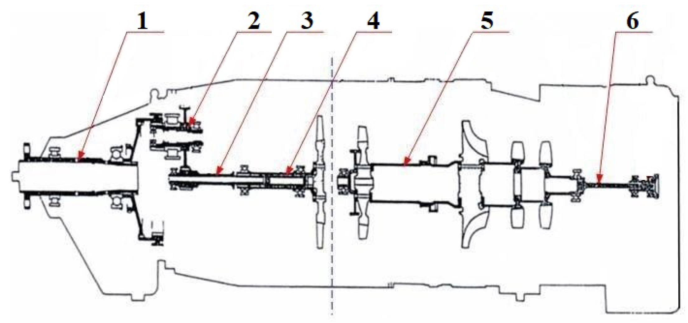
Figure 2.
Distribution of iron concentration.
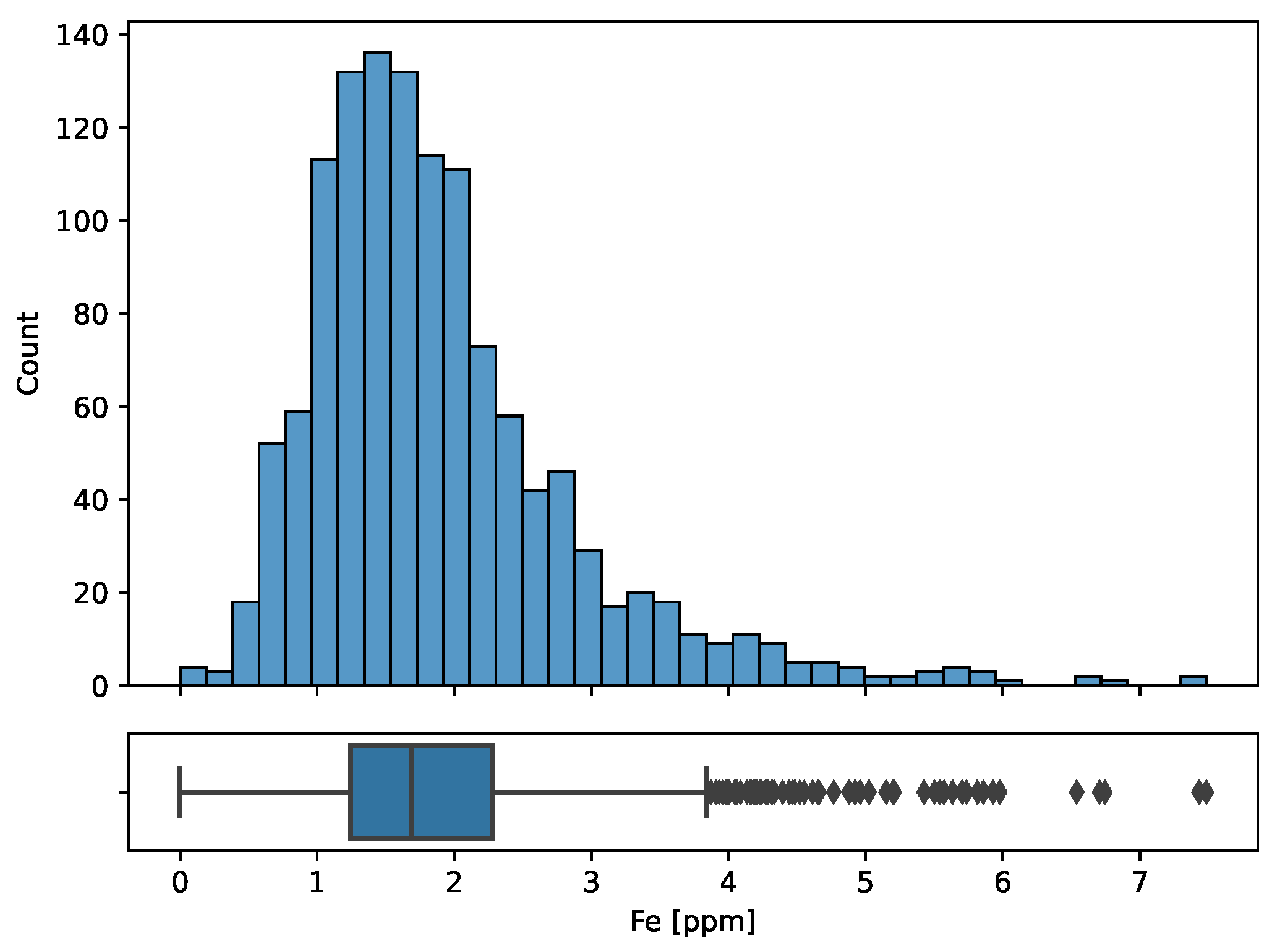
Figure 3.
Distributions of aluminum and zinc concentration.
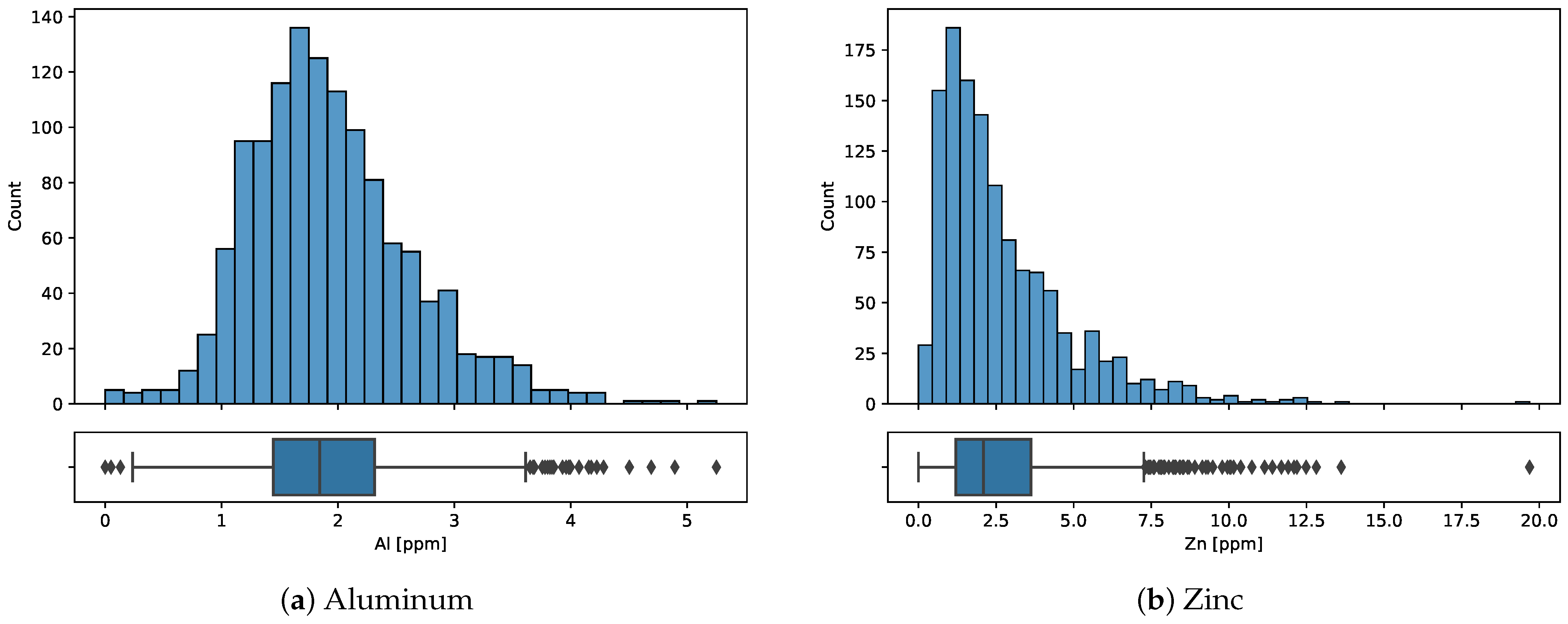
Figure 4.
Iron concentration vs aluminum and zinc.
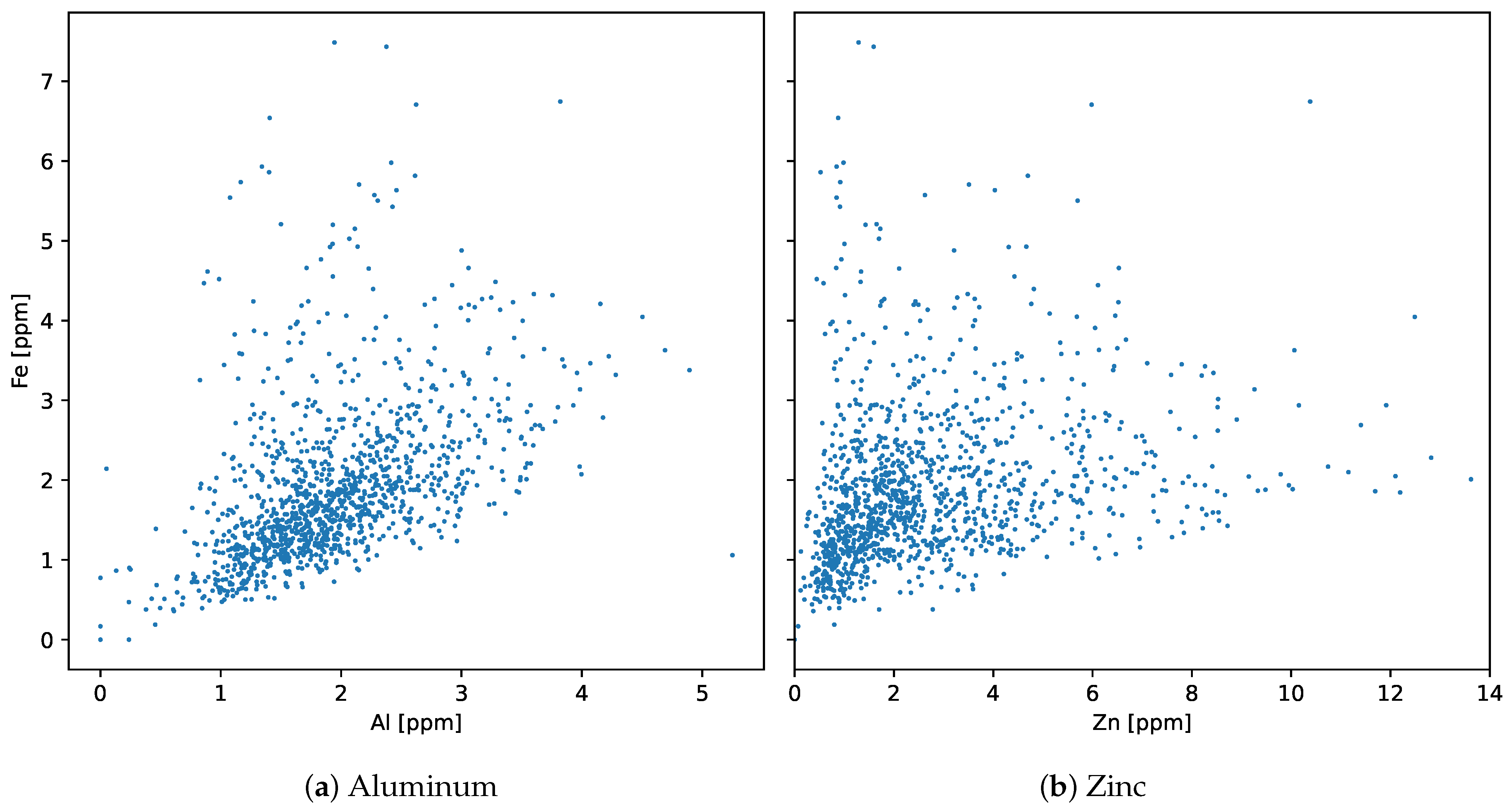
Figure 5.
Probability of variance homogeneity as a function of b parameter for four groups.

Figure 6.
Distributions of iron concentration for individual aluminum and zinc levels before removing outliers and logarithmic transformation.
Figure 6.
Distributions of iron concentration for individual aluminum and zinc levels before removing outliers and logarithmic transformation.
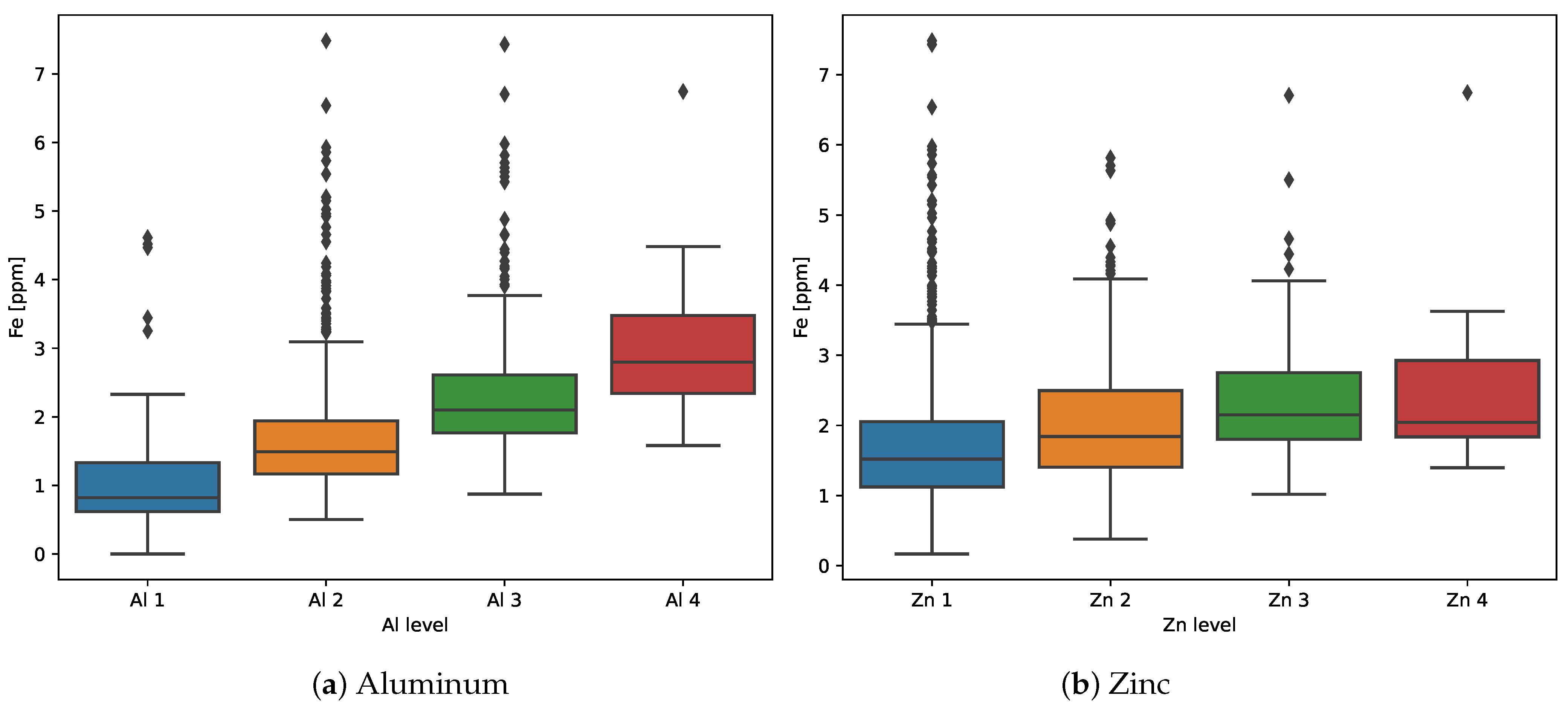
Figure 7.
Grouped boxplot of transformed iron concentration.
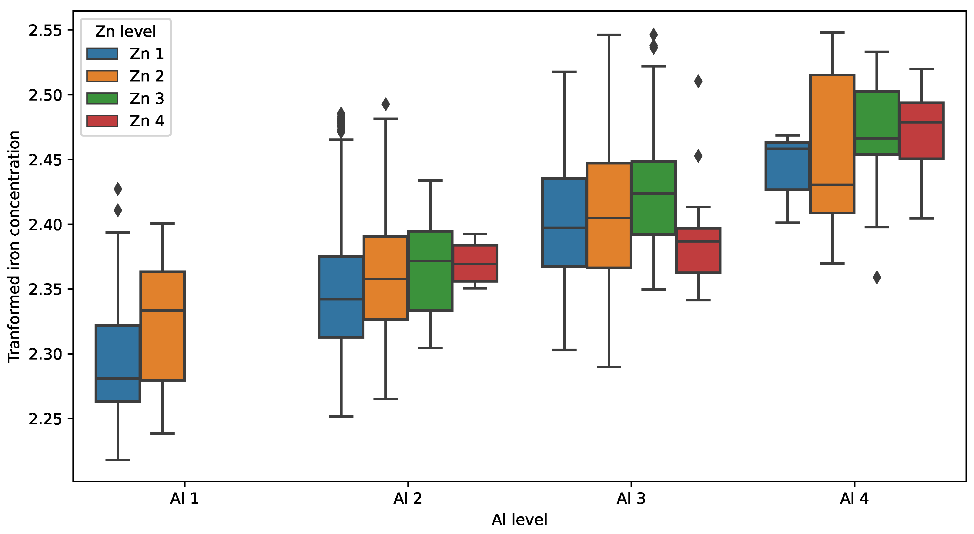
Figure 8.
Interaction plot - the concentration of iron vs aluminum and zinc level.
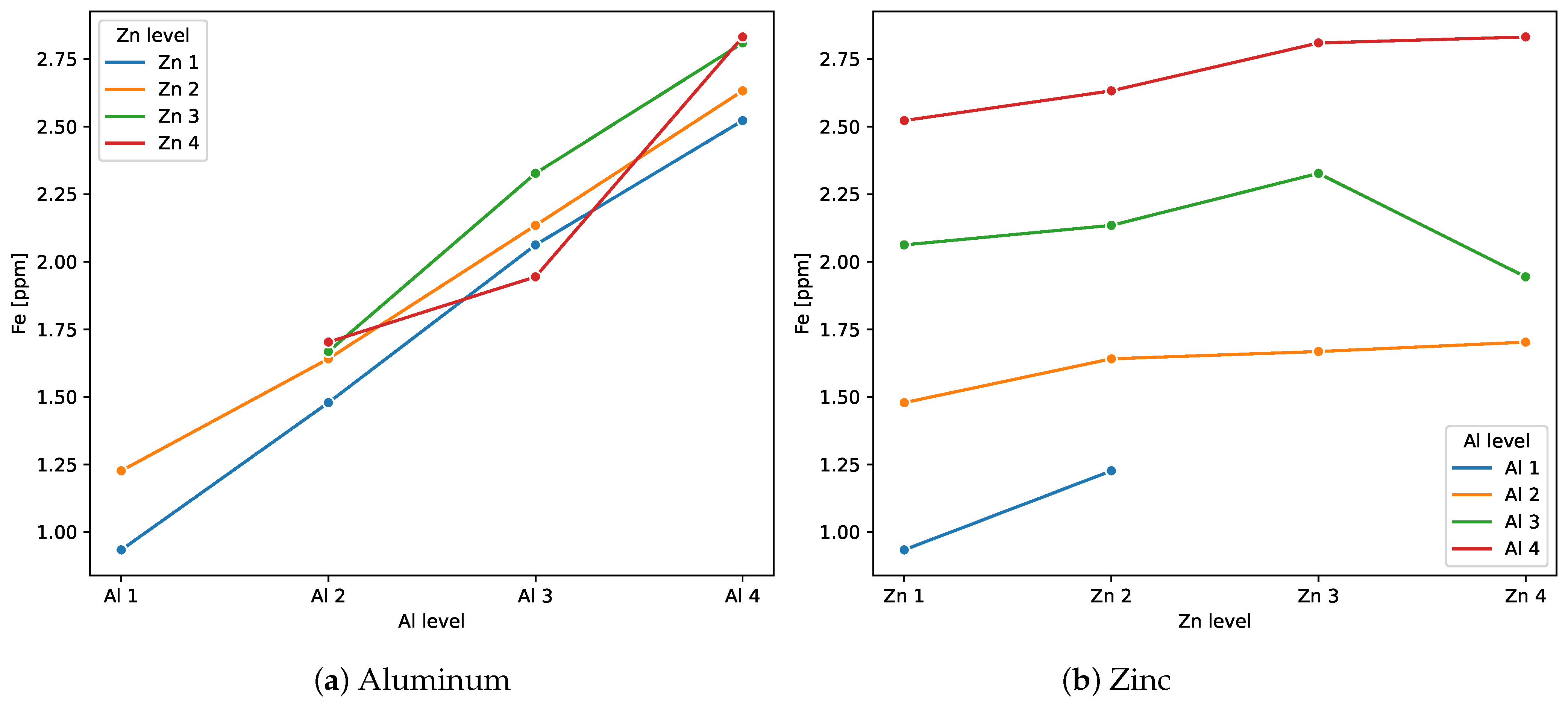
Figure 9.
Engine 1 - iron concentration vs aluminum or zinc concentration with the upper limit of iron for individual groups.
Figure 9.
Engine 1 - iron concentration vs aluminum or zinc concentration with the upper limit of iron for individual groups.
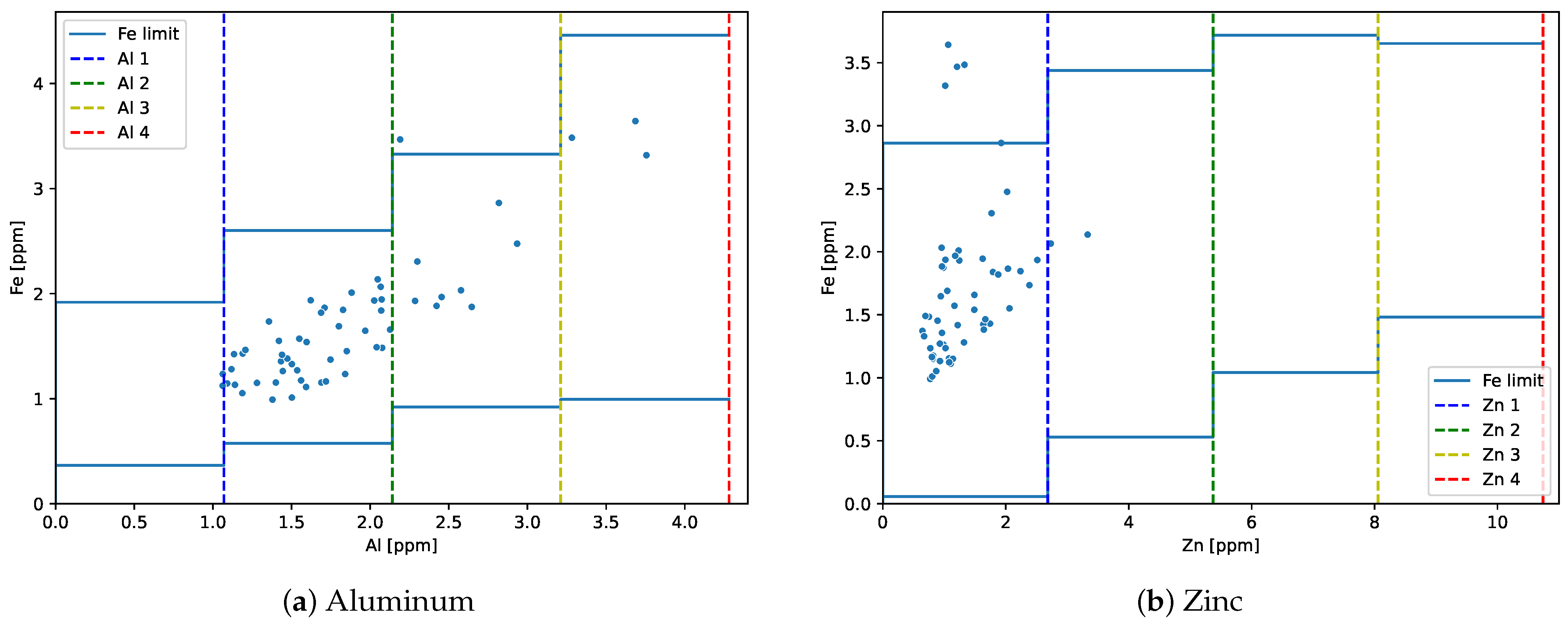
Figure 10.
Engine 1 - concentration time series.
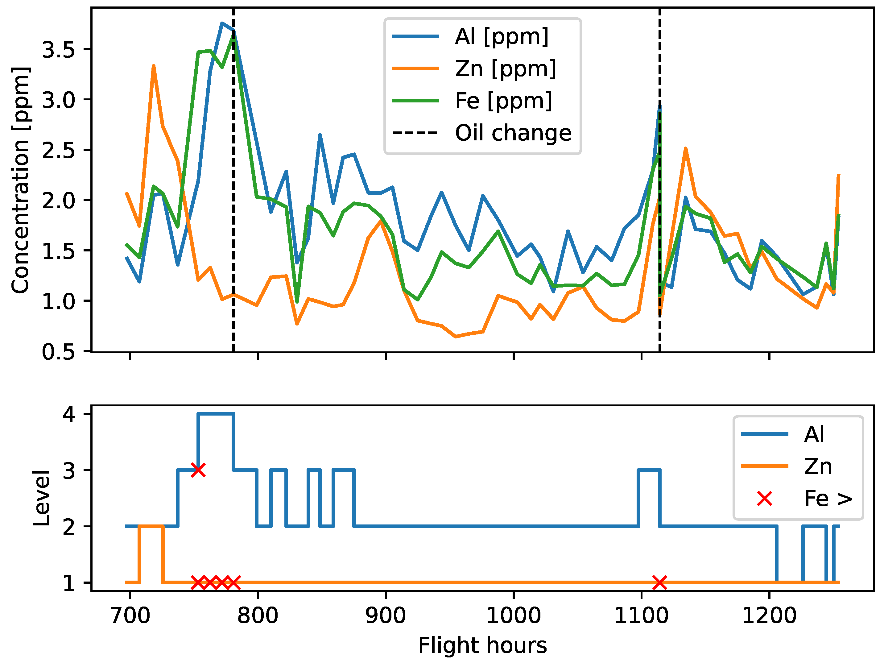
Figure 11.
Iron concentration as a function of aluminum concentration with marked values of the upper limits of the levels and the upper values of iron for individual levels.
Figure 11.
Iron concentration as a function of aluminum concentration with marked values of the upper limits of the levels and the upper values of iron for individual levels.
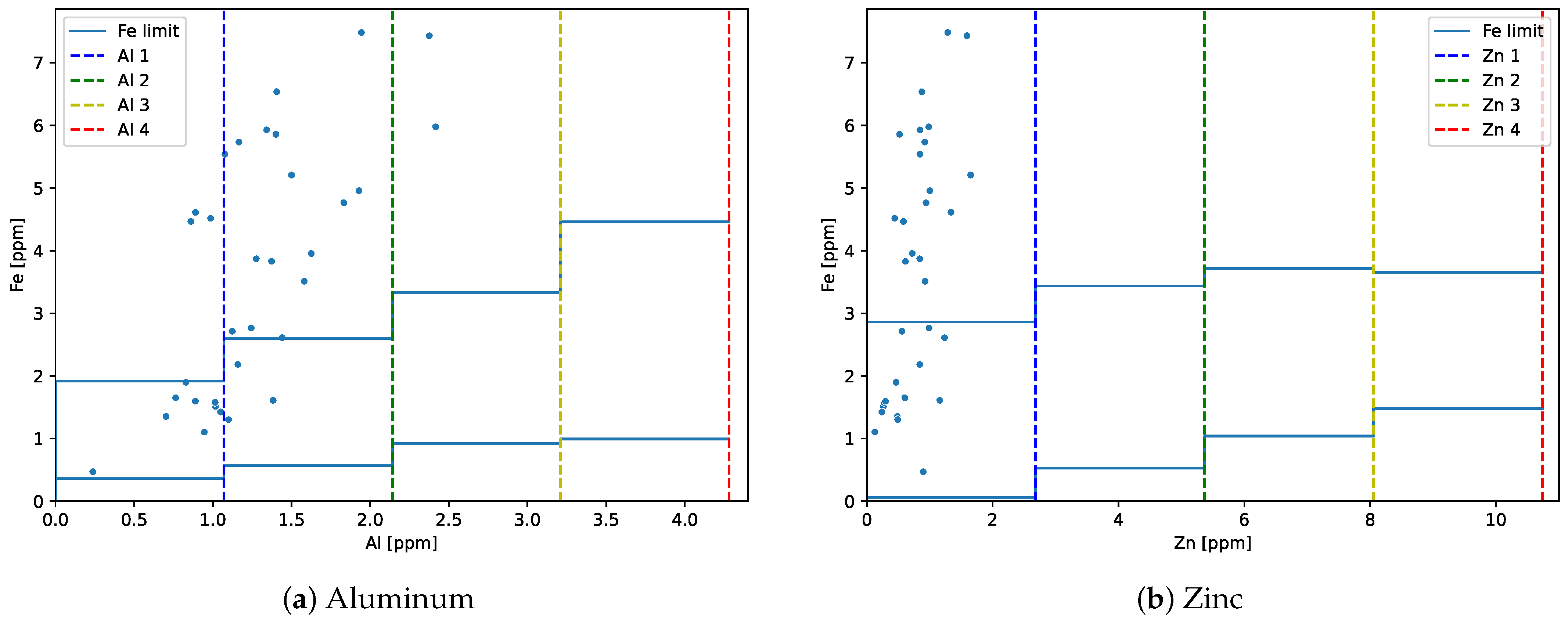
Figure 12.
Iron concentration as a function of flight hours.
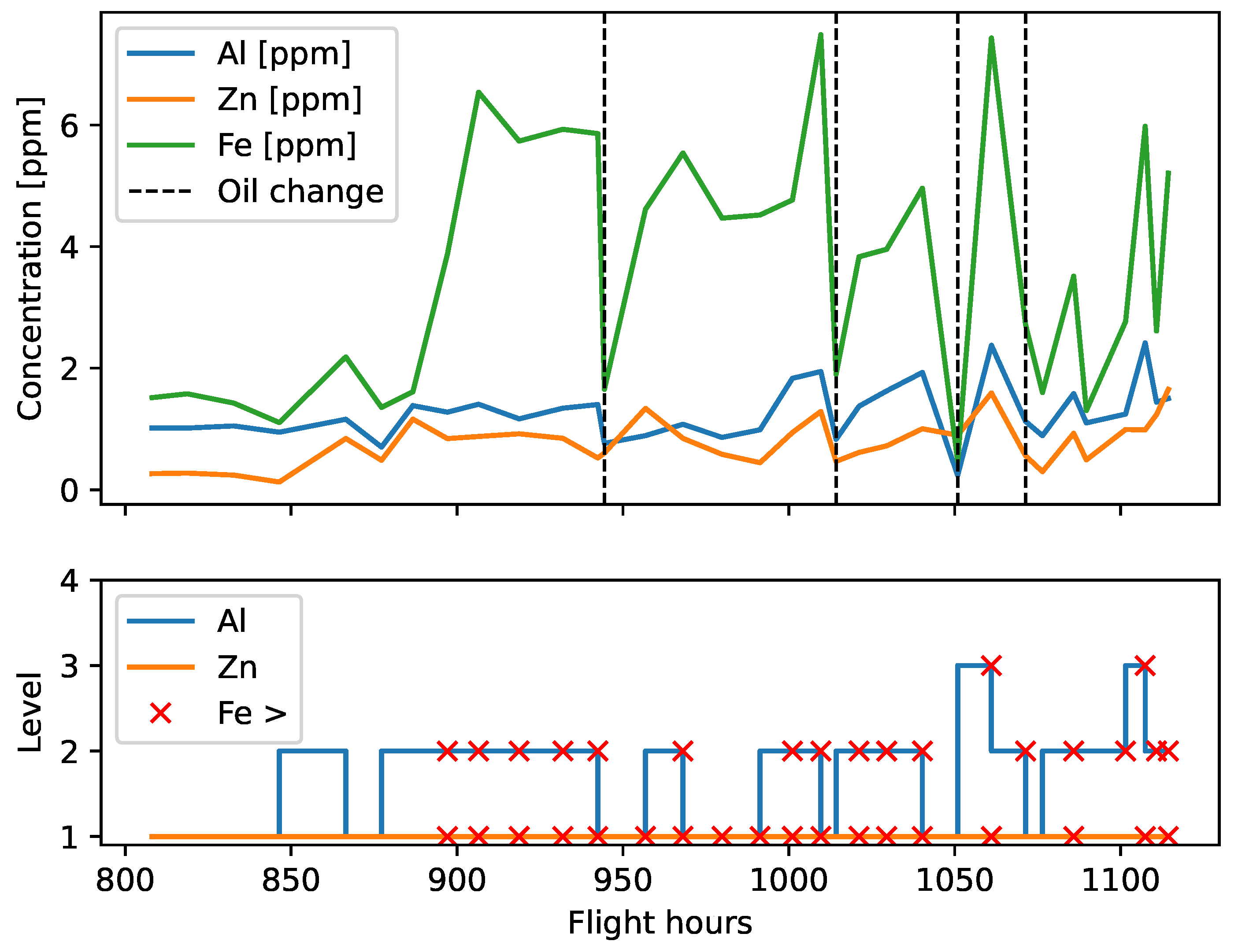
Figure 13.
Engine 2: a) numerous metallic particles on the magnetic plug of AGB, b) hairy chips up to 3 cm long on the filter of the propeller reduction unit.
Figure 13.
Engine 2: a) numerous metallic particles on the magnetic plug of AGB, b) hairy chips up to 3 cm long on the filter of the propeller reduction unit.
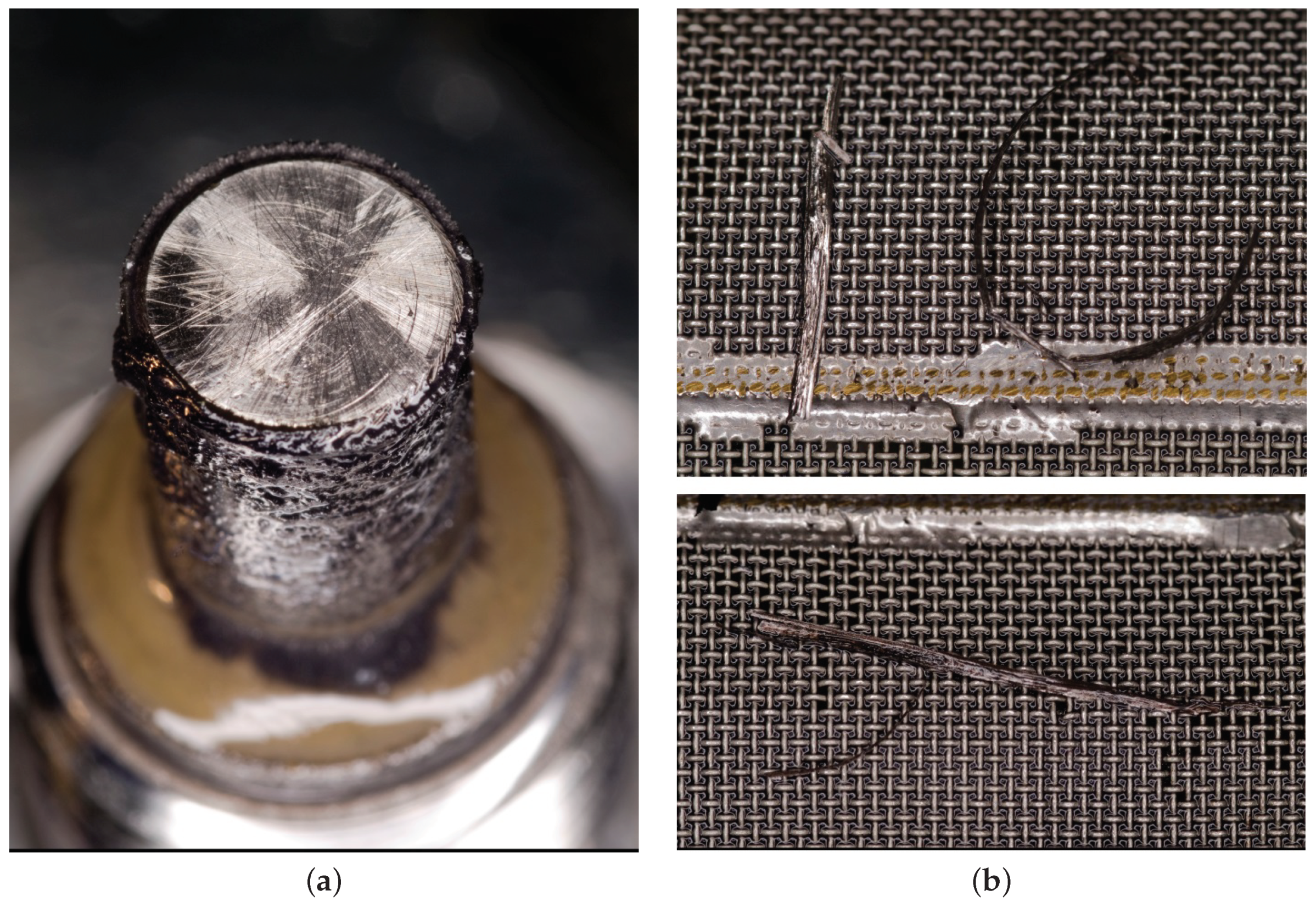

Table 1.
Pearson correlation coefficients.
| Fe [ppm] | Al [ppm] | Zn [ppm] | |
|---|---|---|---|
| Fe [ppm] | 1.00 | 0.46 | 0.25 |
| Al [ppm] | 0.46 | 1.00 | 0.53 |
| Zn [ppm] | 0.25 | 0.53 | 1.00 |
Table 2.
Bartlett’s and Levene’s probabilities for the increasing number of groups.
| Number of groups | |||||||||
| Test | 2 | 3 | 4 | 5 | 6 | 7 | 8 | 9 | 10 |
| Al Bartlett | 0.6068 | 0.0030 | 0.4883 | 0.0002 | 0.0000 | 0.0000 | 0.0000 | 0.0000 | 0.0000 |
| Al Levene | 0.5458 | 0.0009 | 0.4244 | 0.0000 | 0.0000 | 0.0001 | 0.0000 | 0.0004 | 0.0000 |
| Zn Bartlett | 0.9254 | 0.4547 | 0.6357 | 0.1212 | 0.0024 | 0.0000 | 0.0017 | 0.0000 | 0.0000 |
| Zn Levene | 0.9871 | 0.4159 | 0.5858 | 0.0536 | 0.0001 | 0.0000 | 0.0004 | 0.0000 | 0.0000 |
Table 3.
Distribution normality tests for two aluminum and zinc levels.
| Group | Test | Result | Significance |
|---|---|---|---|
| Lillieforsa | 1 | 0.001 | |
| Al 1 | Jarque-Bera | 1 | 0.001 |
| 1 | 0 | ||
| Lillieforsa | 0 | 0.062 | |
| Al 2 | Jarque-Bera | 0 | 0.1341 |
| 0 | 0.0554 | ||
| Lillieforsa | 1 | 0.001 | |
| Zn 1 | Jarque-Bera | 1 | 0.001 |
| 1 | 0 | ||
| Lillieforsa | 1 | 0.0122 | |
| Zn 2 | Jarque-Bera | 0 | 0.0655 |
| 0 | 0.1512 |
Table 4.
Bartlett’s and Levene’s probabilities for transformed data.
| Number of groups | |||||||||
| Test | 2 | 3 | 4 | 5 | 6 | 7 | 8 | 9 | 10 |
| Al Bartlett | 0.5621 | 0.5785 | 0.9791 | 0.2841 | 0.4005 | 0.4583 | 0.5724 | 0.0168 | 0.0542 |
| Al Levene | 0.5005 | 0.4648 | 0.9563 | 0.1432 | 0.2624 | 0.3440 | 0.3065 | 0.2847 | 0.0012 |
| Zn Bartlett | 0.9582 | 0.5488 | 0.9132 | 0.8641 | 0.0227 | 0.0069 | 0.0608 | 0.0006 | 0.0010 |
| Zn Levene | 0.9758 | 0.4472 | 0.8814 | 0.8177 | 0.0082 | 0.0061 | 0.0293 | 0.0005 | 0.0001 |
| b parameter | 170.0 | 3.5 | 9.0 | 5.0 | 2.0 | 1.5 | 1.5 | 1.5 | 1.0 |
Table 5.
Defined aluminum and zinc levels and corresponding transformed iron values.
| Boundaries [ppm] | Observations | Transformed Fe | ||||
| Group | Left | Right | Count | Outliers | Mean | Std |
| Al 1 | 0.0000 | 1.0704 | 90 | 5 | 2.29693 | 0.0468 |
| Al 2 | 1.0704 | 2.1408 | 741 | 48 | 2.35268 | 0.0492 |
| Al 3 | 2.1408 | 3.2112 | 348 | 24 | 2.40928 | 0.0513 |
| Al 4 | 3.2112 | 4.2816 | 64 | 1 | 2.47459 | 0.0625 |
| Zn 1 | 0.0000 | 2.6856 | 779 | 48 | 2.35518 | 0.0591 |
| Zn 2 | 2.6856 | 5.3712 | 321 | 14 | 2.38994 | 0.0654 |
| Zn 3 | 5.3712 | 8.0569 | 108 | 5 | 2.41880 | 0.0621 |
| Zn 4 | 8.0569 | 10.7425 | 31 | 1 | 2.41990 | 0.0590 |
Table 6.
Tests for distribution normality of transformed iron data for individual Al and Zn levels.
| Test | Group | Result | Significance | Group | Result | Significance |
|---|---|---|---|---|---|---|
| Lillieforsa | 1 | 0.0010 | 0 | 0.0520 | ||
| Jarque-Bera | Al 1 | 0 | 0.0708 | Zn 1 | 1 | 0.0068 |
| 1 | 0.0023 | 1 | 0.0003 | |||
| Lillieforsa | 1 | 0.0010 | 1 | 0.0451 | ||
| Jarque-Bera | Al 2 | 0 | 0.0511 | Zn 2 | 1 | 0.0425 |
| 1 | 0.0005 | 0 | 0.0641 | |||
| Lillieforsa | 0 | 0.1665 | 0 | 0.3512 | ||
| Jarque-Bera | Al 3 | 0 | 0.0793 | Zn 3 | 0 | 0.2220 |
| 0 | 0.3232 | 0 | 0.3341 | |||
| Lillieforsa | 0 | 0.3315 | 0 | 0.2529 | ||
| Jarque-Bera | Al 4 | 0 | 0.4094 | Zn 4 | 0 | 0.1572 |
| 0 | 0.3141 | 1 | 0.0110 |
Table 7.
Two-way ANOVA without interaction effects.
| Source | Sum Sq. | d.f. | F | Prob>F | Effect Size |
|---|---|---|---|---|---|
| Al | 1.063465 | 3 | 149.088665 | 1.885264e-81 | 0.278545 |
| Zn | 0.055779 | 3 | 7.819726 | 3.615759e-05 | 0.014610 |
| Residual | 2.698691 | 1135 |
Table 8.
Two-way ANOVA with interactions after removing Al 1 level.
| Source | Sum Sq. | d.f. | F | Prob>F | Effect size |
|---|---|---|---|---|---|
| Al | 0.734975 | 2 | 153.271682 | 4.261817e-59 | 0.226810 |
| Zn | 0.052767 | 3 | 7.335961 | 7.214323e-05 | 0.020626 |
| Al*Zn | 0.012550 | 6 | 0.872404 | 5.145026e-01 | 0.004984 |
| Residual | 2.505514 | 1045 |
Table 9.
LSD and Bonferroni’s test results and their confidence intervals (CI) for Al concentration levels.
Table 9.
LSD and Bonferroni’s test results and their confidence intervals (CI) for Al concentration levels.
| Compared | CI left | LSD test | CI right | CI left | Bonferroni | CI right | |
| groups | boundary | result | boundary | boundary | result | boundary | |
| Al 1 | Al 2 | -0.0690 | -0.0588 | -0.0486 | -0.0725 | -0.0588 | -0.0451 |
| Al 1 | Al 3 | -0.1239 | -0.1130 | -0.1022 | -0.1276 | -0.1130 | -0.0984 |
| Al 1 | Al 4 | -0.1790 | -0.1623 | -0.1457 | -0.1848 | -0.1623 | -0.1399 |
| Al 2 | Al 3 | -0.0604 | -0.0542 | -0.0481 | -0.0625 | -0.0542 | -0.0459 |
| Al 2 | Al 4 | -0.1176 | -0.1035 | -0.0895 | -0.1225 | -0.1035 | -0.0846 |
| Al 3 | Al 4 | -0.0639 | -0.0493 | -0.0348 | -0.0689 | -0.0493 | -0.0297 |
Table 10.
Scheffe’s and Tukey’s test results and their confidence intervals (CI) for Al concentration levels.
Table 10.
Scheffe’s and Tukey’s test results and their confidence intervals (CI) for Al concentration levels.
| Compared | CI left | Scheffe | CI right | CI left | Tukey | CI right | |
| groups | boundary | result | boundary | boundary | result | boundary | |
| Al 1 | Al 2 | -0.0733 | -0.0588 | -0.0443 | -0.0721 | -0.0588 | -0.0455 |
| Al 1 | Al 3 | -0.1285 | -0.1130 | -0.0975 | -0.1272 | -0.1130 | -0.0988 |
| Al 1 | Al 4 | -0.1861 | -0.1623 | -0.1386 | -0.1841 | -0.1623 | -0.1405 |
| Al 2 | Al 3 | -0.0630 | -0.0542 | -0.0454 | -0.0623 | -0.0542 | -0.0461 |
| Al 2 | Al 4 | -0.1236 | -0.1035 | -0.0835 | -0.1219 | -0.1035 | -0.0851 |
| Al 3 | Al 4 | -0.0701 | -0.0493 | -0.0286 | -0.0684 | -0.0493 | -0.0303 |
Table 11.
LSD and Bonferroni’s test results and their confidence intervals (CI) for Zn concentration levels.
Table 11.
LSD and Bonferroni’s test results and their confidence intervals (CI) for Zn concentration levels.
| Compared | CI left | LSD test | CI right | CI left | Bonferroni | CI right | |
| groups | boundary | result | boundary | boundary | result | boundary | |
| Zn 1 | Zn 2 | -0.0380 | -0.0305 | -0.0231 | -0.0406 | -0.0305 | -0.0205 |
| Zn 1 | Zn 3 | -0.0706 | -0.0590 | -0.0474 | -0.0746 | -0.0590 | -0.0434 |
| Zn 1 | Zn 4 | -0.0868 | -0.0667 | -0.0465 | -0.0937 | -0.0667 | -0.0396 |
| Zn 2 | Zn 3 | -0.0410 | -0.0285 | -0.0159 | -0.0454 | -0.0285 | -0.0115 |
| Zn 2 | Zn 4 | -0.0568 | -0.0361 | -0.0154 | -0.0640 | -0.0361 | -0.0082 |
| Zn 3 | Zn 4 | -0.0302 | -0.0076 | 0.0149 | -0.0380 | -0.0076 | 0.0227 |
Table 12.
Scheffe’s andTukey’s test results and their confidence intervals (CI) for Zn concentration levels.
Table 12.
Scheffe’s andTukey’s test results and their confidence intervals (CI) for Zn concentration levels.
| Compared | CI left | Scheffé | CI right | CI left | Tukey | CI right | |
| groups | boundary | result | boundary | boundary | result | boundary | |
| Zn 1 | Zn 2 | -0.0412 | -0.0305 | -0.0199 | -0.0403 | -0.0305 | -0.0208 |
| Zn 1 | Zn 3 | -0.0756 | -0.0590 | -0.0425 | -0.0742 | -0.0590 | -0.0438 |
| Zn 1 | Zn 4 | -0.0954 | -0.0667 | -0.0380 | -0.0930 | -0.0667 | -0.0403 |
| Zn 2 | Zn 3 | -0.0464 | -0.0285 | -0.0105 | -0.0449 | -0.0285 | -0.0120 |
| Zn 2 | Zn 4 | -0.0656 | -0.0361 | -0.0066 | -0.0632 | -0.0361 | -0.0090 |
| Zn 3 | Zn 4 | -0.0398 | -0.0076 | 0.0245 | -0.0371 | -0.0076 | 0.0218 |
Table 13.
Concentration of aluminum and zinc and the corresponding iron concentration limits.
| Lower limit | Upper limit | Fe lower limit | Fe upper limit | |
| Interval | (ppm) | (ppm) | (ppm) | (ppm) |
| AL 1 | 0.0000 | 1.0704 | 0.0559 | 1.9183 |
| AL 2 | 1.0704 | 2.1408 | 0.5279 | 2.6015 |
| AL 3 | 2.1408 | 3.2112 | 1.0416 | 3.3275 |
| AL 4 | 3.2112 | 4.2816 | 1.4807 | 4.4589 |
| ZN 1 | 0.0000 | 2.6856 | 0.365 | 2.8625 |
| ZN 2 | 2.6856 | 5.3712 | 0.5748 | 3.4378 |
| ZN 3 | 5.3712 | 8.0569 | 0.9207 | 3.7174 |
| ZN 4 | 8.0569 | 10.7425 | 0.9933 | 3.6528 |
Disclaimer/Publisher’s Note: The statements, opinions and data contained in all publications are solely those of the individual author(s) and contributor(s) and not of MDPI and/or the editor(s). MDPI and/or the editor(s) disclaim responsibility for any injury to people or property resulting from any ideas, methods, instructions or products referred to in the content. |
© 2023 by the authors. Licensee MDPI, Basel, Switzerland. This article is an open access article distributed under the terms and conditions of the Creative Commons Attribution (CC BY) license (http://creativecommons.org/licenses/by/4.0/).
Copyright: This open access article is published under a Creative Commons CC BY 4.0 license, which permit the free download, distribution, and reuse, provided that the author and preprint are cited in any reuse.


