Submitted:
07 June 2023
Posted:
08 June 2023
You are already at the latest version
Abstract
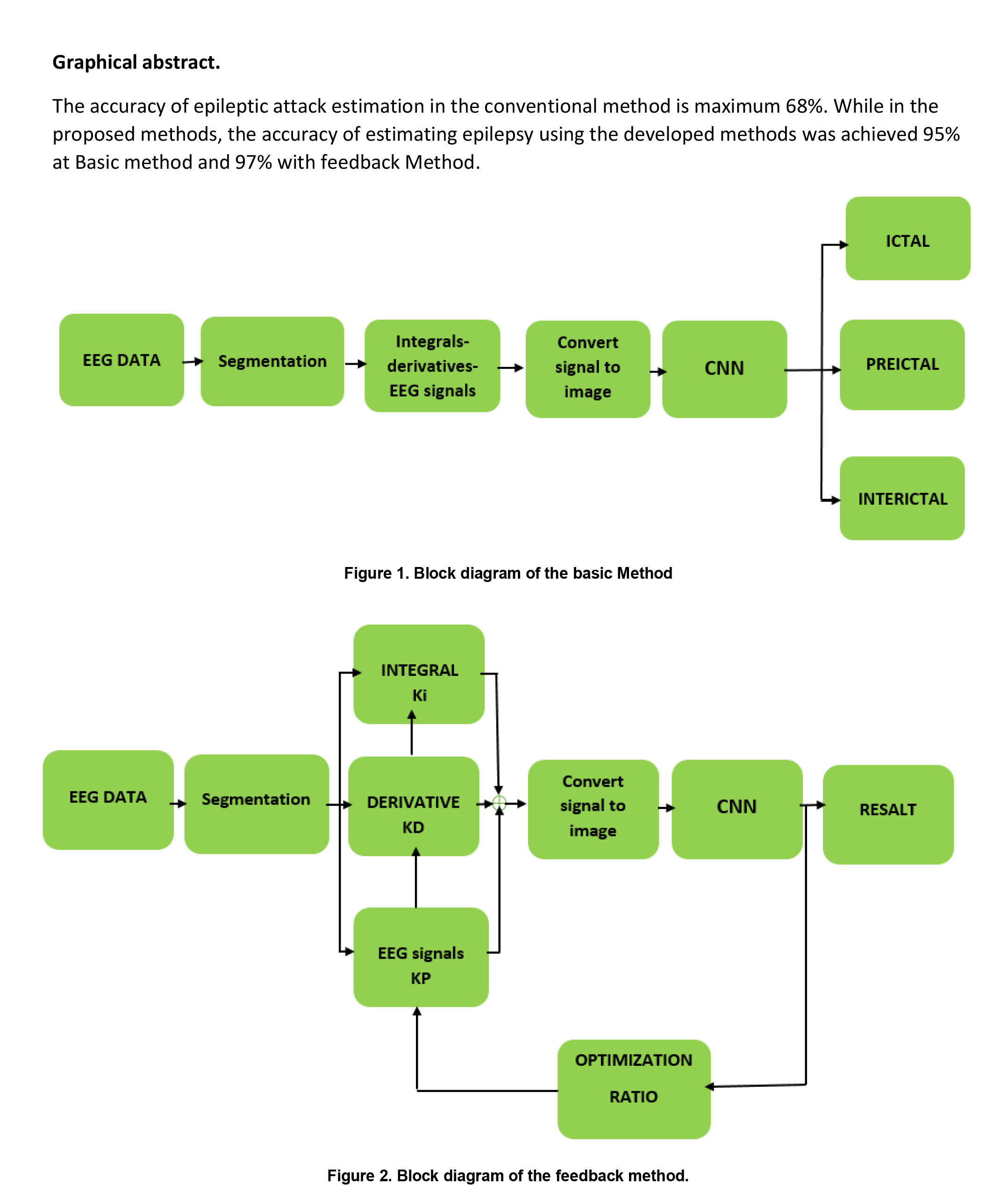
Epilepsy is a neurological disorder that affects approximately 1% of the world's population. To diagnose and estimate the occurrence of epilepsy, the analysis of recorded brain activity is performed by a neurologist, which is not only time-consuming and tedious but also occasionally accompanied by human error. Therefore, in recent decades, researchers have aimed to unravel an approach for designing and building an automated method for diagnosing and estimating the occurrence of epilepsy. Accordingly, the present study proposed two new-fangled ways based on brain signals and a convolutional neural network (CNN). Moreover, this research implements a CNN with a sequential three-layer structure. Numerous experiments were performed, and the accuracy of estimating epilepsy using the developed methods was achieved at 95% without feedback and 97% with feedback. The proposed methods were proven to be more accurate than the previous techniques and can be employed as a physician's assistant once entering the field of operation.
Keywords:
Epilepsy
; Electroencephalogram
; Convolutional neural networks
; Brain signal integral
; Brain signal derivative
1. Introduction
Epileptic seizures are a significant problem, affecting approximately 70 million individuals worldwide [1]. Currently, the disease is controlled and treated with medications in mild cases, and with surgery in acute ones. However, no definitive therapy is available yet [2,3]. Patients with epilepsy cope with harmful risks in daily life (e.g., driving, sleeping, and doing daily activities) [4,5,6]. Predicting epilepsy can prodigiously aid individuals with epilepsy [7]. Using Electroencephalography (EEG) to study brain signals is simpler and cheaper than the other methods [8,9,10]. The traditional method of studying brain signals is complex, time-consuming, and error-prone [11]. Despite the introduction of novel techniques for diagnosing epileptic seizures, their clinical use has not yet been reported [12]. The epileptic patients’ brain signals are divided into ictal and inter-ictal [13]. Besides, in the classifiers’ section, classifier types such as Support Vector Machine (SVM), Sparse Representation classification (SRC), the K-Nearest Neighbor (KNN), and the Multilayer Perceptron (MLP) are employed [14,15]. In older techniques, statistical properties were used as attributes, including mean, standard deviation, median, irregularity, elongation, skewness, and signal energy [16,17,18]. Another technique proposes creating 3D images of brain signals and applying them to a CNN to diagnose and estimate epileptic seizures [19]. In recent studies, using a CNN has been widespread in diagnosing and estimating epileptic seizures. To increase the accuracy of this method, functions were used before the CNN. Such functions have significantly increased these methods’ accuracy from 58% to about 93%. The so-called principle functions embrace the use of Principal Component Analysis (PCA) and Independent Component Analysis (ICA) [20]. Another utilized function before the CNN is the Fast Fourier transform function [21]. An additional central technique was the time-frequency domain conversion [22,23]. The Reconstructed Phase Space (RPS) technique is the other critical utilized function before the CNN [24]. The Pearson correlation coefficient and maximum information coefficient were the other functions used to increase the method’s accuracy in such studies [25]. Zuyi Yu et al. used a Local Mean Analysis (LMD) before CNN to extract the feature [26]. Jana. R et al. generated sub-signals with a sampling time of 1 second to test and train the CNN [27]. S. Muhammad Usman et al. used the time-frequency domain conversion as a primary feature to increase the accuracy of the algorithm [28]. In the study of Abdulnasir Yildiza et al., the domain-time conversion of brain signals along with class activation mapping of brain signals was used [29]. Zuochen Wei et al. reported the initial feature by using the maximum and minimum points of brain signals called MIDS prior to the CNN [30]. S. Raghu et al. used frequency spectrum as a primary feature before CNN [31]. S. R. Ashokkumar et al. exploited two different primary functions, including time-frequency conversion and entropy as two primary features before the CNN with the intention of diagnosing epileptic seizures [32]. J. Lian et al. used the relationship between different channels signals as a primary feature [33]. In the reviewed sources, applying a function prior to the CNN augmented the accuracy by approximately 58% and the accuracy with the numerical value of 93% has been reported. Since accessing the accuracy of more than 93% was a demanding challenge to overcome in the above-mentioned studies, a newly proposed method is presented. In the present paper, by using brain signals, a combined function incorporating integral signal, derivative signal, and the main signal itself before the CNN were utilized with the intention of automatic detection and estimation of epileptic seizures and enhancing the accuracy of the method. In the current investigation, the output of the hybrid function included an integral signal with KI coefficient and derivative signal with KD coefficient, as well as the signal itself with KP coefficient. However, these coefficients were selected as variables to achieve maximum accuracy. Thenceforth, after selecting the so-called coefficients and magnifying the differences in the three states of brain signals using the stated hybrid function, a CNN was employed to create the final feature and decision.
2. Materials and Methods
In the present section, the exploited database in the current study will be examined and the mathematical background related to the convolutional neural networks will be presented.
2.1. DATA
In the present inquiry, Brain signals were used from the Massachusetts Institute of Technology database (MIT, USA), which includes data of the 16 participants with 23 channels, with a sampling frequency of 256 Hz. From the so-called 16 participants, 11 were female and 5 male. Epileptic seizures occurred for several minutes during the recording of brain signals in 16 participants. The age range of females was between 1.5-19 years and for the males was 3-22 years. For each of the selected data, the onset and ending time of the epileptic seizure has been determined, which is different for each participant in the test. The brain signals with a sampling time of 1 second of the subjects were divided into 3 classes, including ictal, pre-ictal, and inter-ictal. Besides, the number of samples to be tested were equally selected for all three modes (i.e., ictal, Pre-ictal, and Inter-ictal).
2.2. Convolutional neural network
The CNN was introduced in 1998 by Fukushima [34]. It was not widely used in the early periods due to hardware and computational limitations for network training. Sermanet et al used the CNN in 2013 for large-scale imaging and film detection [35]. In recent years, convolutional neural networks were extensively used in studies of brain signals, including the prediction of epileptic seizures [36]. The CNN is designed and configured in accordance with the input information of the neural network in various respects, incorporating one-dimensional, two-dimensional, and in some cases three-dimensional. In this configuration, the input data is applied to the neural network as an n × m image. The above neural network consists of three main layers embracing the convolutional layer, Max Pooling Layer, and fully connected layer. The structure of each of these layers will be described in the following sections.
2.2.1. Convolution Layer
In the convolutional layer, the input images to the neural network were swept with a kernel. The dimensions of the kernels vary according to the design and were selected as 3 × 3 and sometimes 5 × 5. In the above layer, images were created from the input image according to the number of selected filters as a feature. In most neural network architectures, 32 filters were selected. But in this study, to reduce the computational load, after a trial and error, 8 filters were selected. In summary, the function of the conventional layer can be expressed by Equation 1, in which is the input matrix and is the output matrix of the conventional layer. Where and are the convolution filter between the n-th offset matrix of the neurons corresponding to the j-th output map. In this regard, f is a nonlinear activation function. The popular activation function are sigmoid, tanh and rectified linear unit (ReLU), etc. in the present work, ReLU is selected for activation function and equation 2 shows the ReLU function.
2.2.2. Max Pooling Layer
In the Max Pooling layer, the image dimensions were reduced. In this layer, the produced images were reduced in the convolutional layer of the sampling. In other words, the dimensions of the images were halved in this layer. The equation 3 is shown rule of the max-pooling layer.
2.2.3. Fully-connected Layer
In the fully connected layer, the properties of the input images were displayed in pixels. Following several convolutional and Max Pooling operations, in the fully-connected layer, the properties appeared as pixels, which were represented as a vector. In the fully connected layer, the created vector was used for the final decision.
2.3. Proposed method
This section describes our proposed method for predicting and diagnosing epileptic seizures, which consists of two separate approaches. The first method, called the Basic suggestion method, is illustrated in Figure 1. To detect and predict epileptic seizures in this method, we utilized a proposed function and a CNN. First, the brain signals were segmented into one-second intervals, and then passed through the proposed function, which is explained in more detail below. The output of the proposed function was then converted into 2D images in the 'convert to image' section, and these images were subsequently fed into the CNN to extract features and make the final decision. To enhance the accuracy and reliability of our approach, we also developed an alternative method called the feedback proposed method, which is depicted in Figure 2. In our proposed method, we utilized feedback from the algorithm's accuracy results to optimize the proposed function by adjusting the values of the proportional coefficients KP, derivative coefficient KD, and integral coefficient Ki. During the pre-ictal state and particularly near the onset of the main epilepsy (ictal state), the frequency of sub-bands of brain signals changes compared to the inter-ictal state. Therefore, it is essential to detect these changes. To accomplish this, we employed a second-order system whose parameters, including KP, KD, and Ki, are automatically adjusted based on the resulting accuracy. The changes to the coefficients continue until the maximum accuracy is attained, at which point the values of KP, KD, and Ki become stable. The output of this system differs for ictal, pre-ictal, and inter-ictal states. Consequently, the resulting images from the output of the system also vary depending on the pre-ictal or inter-ictal state.
2.3.1. Data preprocessing
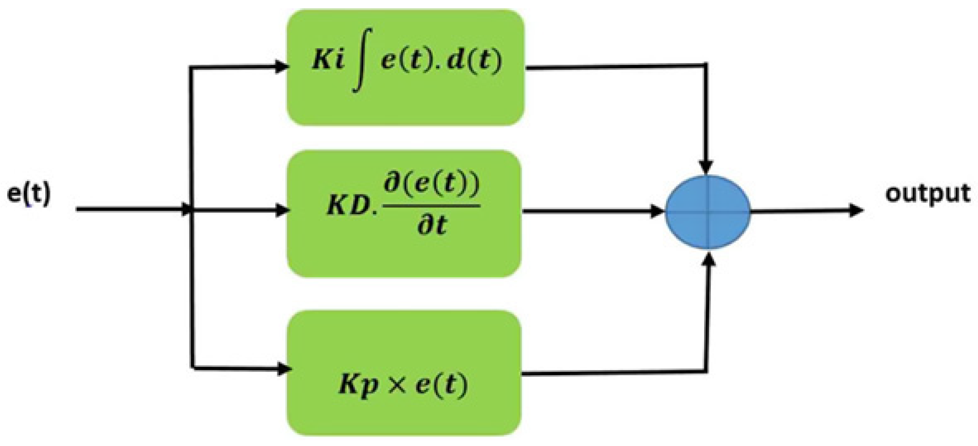
In this section, we describe the preprocessing steps and the performance of the proposed function to prepare the brain signals for the CNN application. Firstly, we extracted brain signals with a duration of 1 second for three modes: Ictal, Pre-ictal, and Inter-ictal, from the Massachusetts Institute of Technology (MIT, USA) database, as shown in Figures 3, 4, and 5. Then, we converted these signals into 2D images using the ‘imagesc (A)' command available in MATLAB software, which displays the 256×23 matrix as an 876×586 image. It should be noted that for each of the mentioned modes, 200 image samples were created for testing. In order to apply these images to the neural network, we resized them to 64×64 dimensions, as shown in Figure 6. To create the initial feature of the segmented brain signals, we passed these signals through the proposed function, as shown in Figure 7. The function consisted of the sum of signal integrals, signal derivatives, and the signal itself, with coefficients Ki, KD, and KP. We used the proposed function to extract the features from the brain signals before applying them to the CNN.
Figure 3.
23 channel signal in ictal mode.
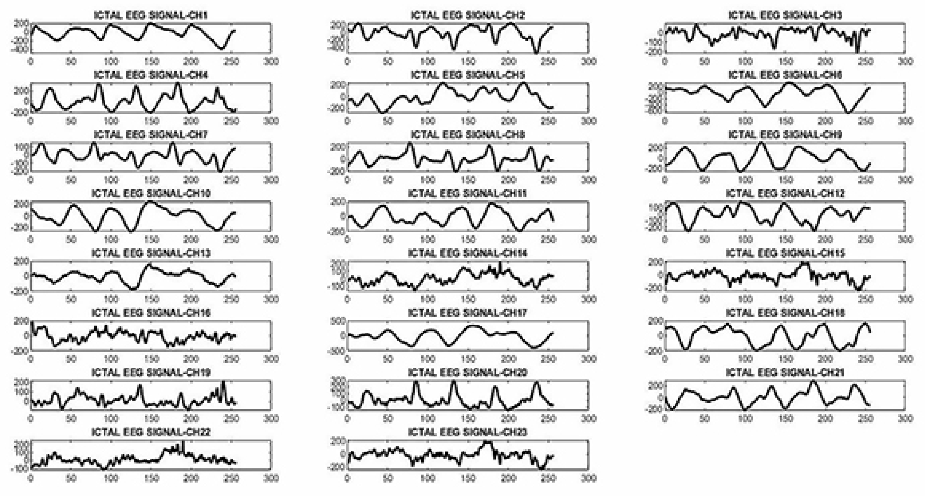
Figure 4.
23 channel signal in pre-ictal mode.
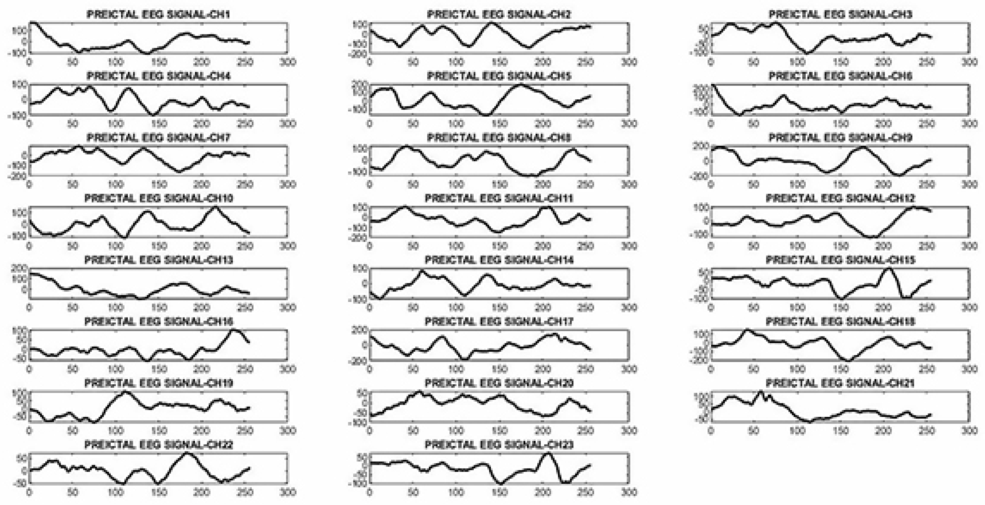
Figure 5.
23 channel signal in inter-ictal mode.
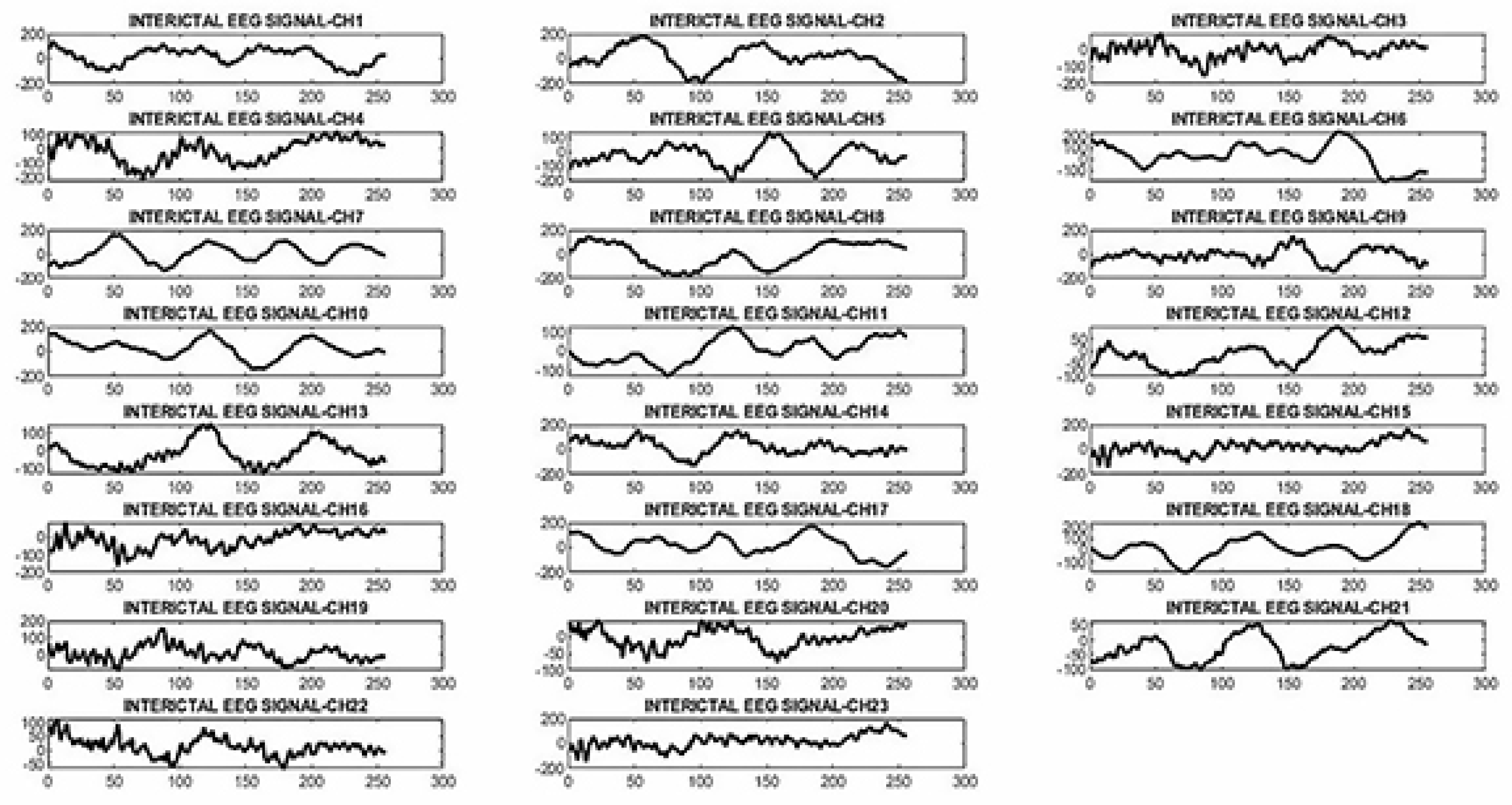
Figure 6.
Images generated from ictal, pre-ictal, and inter-ictal brain signals.
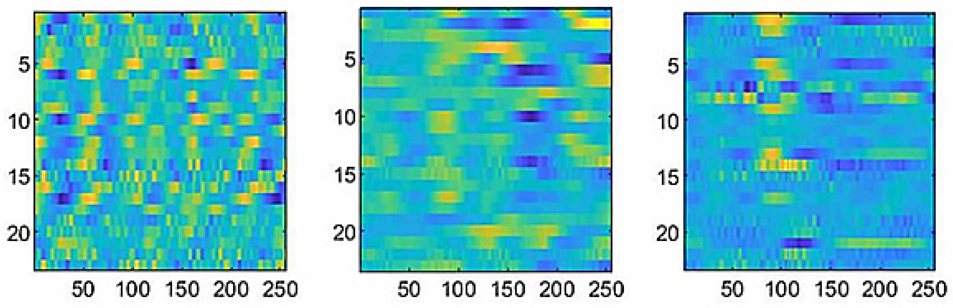
Figure 7.
Block diagram of the proposed function.
2.3.2. Proposed neural network architecture
In the present study, the CNN was used with the structure shown in Figure 8 to extract the features from the images produced by the proposed function and the final decision. The presented structure was obtained through trial and error, and the precise characteristics are shown in Table 1 for each of the convolutional neural networks used in the test. This structure is divided into three parts, each with a convolutional layer and a max pooling layer. In the last part of the architecture, a full connection layer was utilized for the final decision. Moreover, a 3 × 3 mask was used for the convolution of the input images in each of the convolutional layers, and the results of the convolutional classes were then passed through a ReLU function, which benefited from the Arctanh function. At the output of the first part, from the input image with dimensions of 64 × 64, 8 images were produced with dimensions of 64 × 64. Down-sampling operations were performed on the aforementioned images in the following max pooling layer, yielding images with 32 × 32 dimensions. At the output of the second part, from the input image with dimensions of 32 × 32 resulting from the first layer, 16 images with dimensions of 32 × 32 were generated in the convolutional layer. Subsequently, in the max pooling layer, down-sampling operations were performed on the above-stated images, and images with 16 × 16 dimensions were created. In the output of the third part, from the input images with dimensions of 16 × 16 produced in the second layer, 32 images with dimensions of 8 × 8 were produced. The dimensions of the input and output images of each of the above classes are shown in Table 2. In the deep neural network, the results obtained from the third layer included 2048 pixels. However, for the final decision, only 1024 significant pixels have been selected from the total number of pixels.
2.3.3. Data collection training and evaluation
In this part, initially, the data for each of the individuals were divided into 3 modes: ictal, pre-ictal, and inter-ictal, with a 1-second sampling interval. Afterward, the data of the individuals were separately tested with the proposed methods. Next, from the data of 16 individuals, the data of 10 participants were selected whose epileptic seizures were longer than those of other individuals. Subsequently, the data of the 10 participants were combined in two ways: an identical merge and a non-identical merge. In the identical merge mode, 60 samples were selected equally from 10 participants for each of the ictal, pre-ictal, and inter-ictal modes. Finally, 600 sample images were collected for each of the 3 modes. In total, 1800 sample images were selected for each of the three modes mentioned. Figure 9 describes how the test ratio is selected based on the above-stated training. Data were randomly selected from each individual in the non-uniform merging mode, with a different number of samples for each of the three modes mentioned. The test-to-train ratio was selected at 20% to 80%, respectively, for each of the identical and non-identical merges and independent reviews of the data of each participant in the current analysis.
3. Results
In order to improve the accuracy of the method, the images were used as input to the CNN in this study. At the output of the proposed function, 2D images were generated as illustrated in Figure 10.
In order to prove the suggested features for the proposed method and the identical and non-identical merge methods, various tests were performed on the data obtained from patients, the results of which are presented separately to confirm the accuracy of the proposed method compared to other techniques. The tests conducted were generally of three classes and included ictal, pre-ictal, and inter-ictal. The results obtained from the tests of 16 patients were almost the same and therefore, in the following the results obtained from patients’ number 08-21 are presented. In the present study, in order to demonstrate the effects of KP, Ki, and KD coefficients, various experiments were performed on the collected data from the CHB-MIT database, the results of which are shown in Table 3.
The table also shows the results of conventional method tests, which could be useful for comparing with the results of the basic method. In order to determine the influence of each of the mentioned coefficients, various experiments were conducted on one of the samples. In all stages of these experiments, one of the coefficients of the variable was selected and the other coefficients were kept constant. The results of these experiments are shown in Table 4 and Table 5.
Furthermore, in order to compare the results of the patient's classified information, including inter-ictal, ictal, and pre-ictal, the proposed feedback method (Figure 2) was applied, and 97% accuracy was obtained, which indicates an increase of 4% compared to the results of previous studies. Moreover, according to the results of the experiments, the effect of the KD coefficient can be observed on the downloaded information from the CHB-MIT database, and the best case in Table 4 is related to the coefficients KI = 0.6, KP = 0.3, and KD = 0.2. By examining the test results, the effect of the Ki coefficient can be realized on the downloaded information from the CHB-MIT database, the best case of which is shown in Table 5 and is related to the coefficients KP = 0.5, KI = 0.2, and KD = 0.9. The mentioned steps were performed using the feedback method and 97% accuracy was obtained. In the next step, the signals of 10 participants were merged into two identical and non-identical partnerships. Table 6 shows the results of the identical and non-identical participatory integration tests for the base method.
It can be observed in Table 6 that the maximum percentage of identical and non-identical participatory integration for the base method is related to the states KI = KP = 0.1, KD = 2. The mentioned steps were performed using the feedback method. Following the implementation of the feedback method for identical and non-identical participatory integration modes, all different values for KP, Ki, and KD coefficients were automatically tested, and finally, the feedback algorithm determined the maximum accuracy. It is noteworthy that in this evaluation, the maximum accuracy was 95% for the integration of identical participation and 93% for the integration of non-identical participation. The proposed base method is shown in Figure 1. According to this figure, it is evident that the existence of the new function leads to a significant improvement in the accuracy of the method. The feedback proposed method, which is in fact a combination of the feedback and the basic suggestion method, was presented in Figure 2 in order to enhance the performance of the basic structure. The advantages of this method incorporate higher reliability and enhanced accuracy than the conventional method and the proposed basic method. It should be noted that the primary function has not been used in conventional methods and therefore exhibits low accuracy and sensitivity. In order to analyze the data in each of the proposed methods and the conventional method, several testing and training techniques were applied. One of these techniques is the conventional method in which the testing and training of the CNN are considered separately for each participant. The second technique of testing that is applied to the proposed method and the conventional method is the participatory approach of uniform integration of the data of the test subjects. Both the proposed method and the conventional method utilized the same data for the training and testing of neural networks. However, in the participatory method(uniform and non-uniform integration), image data was divided into three classes, including epilepsy, pre-epilepsy, and normal state, and were utilized non-uniformly in the testing and training of convolutional neural network. The main feature of these techniques of identical and non-identical integration is that they make it conceivable for epilepsy diagnosis and prediction methods to be universally available for patients with epileptic seizures. In other words, it prevents the diagnostic device from being proprietary to a particular patient, which diminishes the additional costs associated with designing and manufacturing proprietary equipment. Indubitably, it should be noted that the power of generalization in the non-identical participation method was much greater than the identical integration method in a way that the data of individuals outside the sampling can also be evaluated. Using the results obtained from the application of the developed integration approach on the proposed methods and conventional method, it is observed that the accuracy of the feedback and basic methods was much higher than the conventional method and can be employed in various applications such as clinical therapies and medical diagnostic equipment. Table 7 illustrates a comparison between the results of the proposed method and the conventional method. According to this table, it is observed that under comparable conditions and by using the same participation method, the accuracy of the feedback, basic, and conventional methods is equal to 95%, 91%, and 50%, respectively. It should be noted that conventional methods are those in which no function or filter is used to extract the signal feature and the signal is directly applied to the neural network. However, these results are slightly lower than the ones obtained with a similar method through the application of the non-identical integration method. The accuracy of the feedback, basic, and conventional methods are 93%, 89%, and 47%, respectively. Table 8 exhibits a detailed comparison between the proposed methods and the previous studies. According to the results of Table 8, it is observed that the proposed methods, under the same conditions, including the use of the same database, demonstrated a significant advantage in the values of accuracy, sensitivity, and specificity. The only limitations of the proposed method were the time required for the implementation of the proposed feedback method, which took around 14 hours for training and initial testing, of which 11.2 hours were training time and 2.8 hours were testing time.
4. Discussion
In the present paper, a basic method and a feedback method were proposed for predicting, detecting, and analyzing brain signals in epileptic seizures. In addition to these two methods, two novel testing and training methods were introduced in order to achieve a method of prediction and diagnosis of generalized epileptic seizures called the identical integration participatory method and the non-identical integration participatory method. According to the execution time of the program and the accuracy of the previous experiments, 600 image samples were selected to perform the identical and non-identical integration tests. It should be noted that initially, the different data integration methods have been investigated using the conventional and the base methods. By examining the results, it is clear that the proposed method was able to enhance the response accuracy of the method by intensifying the accuracy by 50%. After reviewing the results of the conventional method, two proposed methods of merging equal and unequal participation were applied to the proposed methods: the basic method, and the feedback method. Examining the results obtained from the experiments, it was shown that compared to the conventional method, both proposed basic and feedback methods led to enhanced results. Furthermore, using the obtained results, it was found that by applying the identical and non-identical participatory methods, the accuracy degree of the conventional method was equal to 50% and 47%, respectively. However, under similar conditions, applying the basic and feedback methods achieved better results. Hence, the accuracy of the basic method was equal to 91% for the identical participation method and 89% for the non-identical participation method. It should be noted that the accuracy of the proposed feedback method by applying the identical method of integration was equal to 95% and for the method of non-identical participation was equal to 93%. These results indicated that the proposed basic method along with the feedback method demonstrated the ability to enhance accuracy. Therefore, they can be used to reduce the error in the epileptic seizure in a short period, as well as the side costs of manufacturing medical equipment. It should also be noted that the main feature of applying the proposed participatory methods was to make it possible to build equipment for predicting and diagnosing epilepsy as a unit for all patients so that the constructed device could be initially trained with the initial data recorded in the computer and subsequently be utilized by the public without any necessity for re-training.
Author Contributions
Conceptualization: G. A; Methodology: G. A; Formal; Analysis and investigation: G. A; Writing—original draft: G. A; Preparation: G. A; Writing—review and editing: G. A, T. Y, S. M; Supervision: G. A, T. Y. All authors have read and agreed to the published version of the manuscript.
Funding
This research received no external funding.
Institutional Review Board Statement
The study was conducted according to the guidelines of the Declaration of Helsinki. Authors declare that in view of the retrospective nature of the study, since all the procedures being performed were part of the routine care, all the collected data were anonym zed, and no information is linked or linkable to a specific person.
Informed Consent Statement
Not applicable.
Data Availability Statement
Brain signals were used from the Massachusetts Institute of Technology database (MIT, USA).
Conflicts of Interest
The authors declare no conflict of interest.
References
- Subasi, A.; Gursoy, M.I. EEG signal classification using PCA, ICA, LDA and support vector machines. Expert Syst Appl. 2010, 37, 8659–66. [Google Scholar] [CrossRef]
- Yan, T.; Geng, Y.; Wu, J.; Li, C. Interactions between multisensory inputs with voluntary spatial attention an fMRI study. Neuroreport. 2015, 26, 605–612. [Google Scholar] [CrossRef]
- López-Hernández, E.; Bravo, J.; Solís, H. Epilepsia y antiepileptic’s de primera y segunda generación. Aspectos básicos útiles en la práctica clínica. Revista De La Facultad De Medicina. Epub ahead of print 2011. [Google Scholar]
- F. Mormann, R. G. Andrzejak et al. Seizure prediction the long and winding road. Brain 2006, 130, 314–333. [Google Scholar] [CrossRef]
- Yan, T.; Zhao, S.; Uono, S.; Bi, X.; Tian, A.; Yoshimura, S. , et al. Target object moderation of attentional orienting by gazes or arrows. Attent. Percep. Psychophys. 2016, 78, 2373–2382. [Google Scholar] [CrossRef]
- P Kwan, M J Brodie (). Early identification of refractory epilepsy. The New England journal of medicine 2000, 342, 314–319. [Google Scholar] [CrossRef] [PubMed]
- J de Tisi, G, S Bell et al. The long-term outcome of adult epilepsy surgery, patterns of seizure remission, and relapse: a cohort study. Lancet (London, England) 2011, 378, 1388–1395. [Google Scholar] [CrossRef]
- Misulis, K, E Atlas of EEG. Seizure Semiology, and Management. New York, NY: Oxford University Press. 2013.
- Pachori, R.B.; Patidar, S. Epileptic seizure classification in EEG signals using second-order difference plot of intrinsic mode functions. Comput. Methods Programs Biomed. 2014, 113, 494–502. [Google Scholar] [CrossRef]
- Litjens, G.; Kooi, T.; Bejnordi, B.E.; Aaa, S.; Ciompi, F.; Ghafoorian, M.; et al. A survey on deep learning in medical image analysis. Med Image Anal. 2017, 42, 60–88. [Google Scholar] [CrossRef]
- Iasemidis, L.D.; Shiau, D.S.; Pardalos, P.M.; Chaovalitwongse, W.; Narayanan, K.; Prasad, A.; et al. Long-term prospective on-line real-time seizure prediction. Clin. Neurophysiol. 2005, 116, 532–544. [Google Scholar] [CrossRef]
- Subasi, A.; Erçelebi, E. Classification of EEG signals using the neural network and logistic regression. Comput Methods Programs Biomed 2005, 78, 87–99. [Google Scholar] [CrossRef] [PubMed]
- Yan, T.; Wang, W.; Liu, T.; Chen, D.; Wang, C.; Li, Y.; et al. Increased local connectivity of brain functional networks during facial processing in schizophrenia: evidence from EEG data. Oncotarget 2017, 8, 63. [Google Scholar] [CrossRef]
- Chengcheng Han. Highly Interactive Brain–Computer Interface Based on Flicker-Free Steady-State Motion Visual Evoked Potential. Scientific Reports 2018, 8, 1. [Google Scholar] [CrossRef]
- S. SHEYKHIVAND, T. YOUSEFI REZAII, Z.MOUSAVI, A. DELPAK. Automatic Identification of Epileptic Seizures from EEG Signals Using Sparse Representation-Based Classification. Published in IEEE Access Journal. 2020, 8, 138834–138845. [Google Scholar] [CrossRef]
- Han, T.; Xu, Z.; Du, J.; Zhou, Q.; Yu, T.; Liu, C.; Wang, Y. Ictal High-Frequency Oscillation for Lateralizing Patients With Suspected Bitemporal Epilepsy Using Wavelet Transform and Granger Causality Analysis. Frontier in Neuroinformatice. 2019, 13, 44. [Google Scholar] [CrossRef]
- Negin Moghim, David W. Predicting Epileptic Seizures in Advance. PLOS ONE. 2014, 10, 3. [Google Scholar] [CrossRef]
- Marzieh Savadkoohi, Timothy Oladunni, Lara Thompson. A machine learning approach to epileptic seizure prediction using Electroencephalogram (EEG) Signal. The Journal of Biocybernetics and Biomedical Engineering 2020, 40, 1328–1341. [Google Scholar] [CrossRef]
- Wei, X.; Zhou, L.; Chen, Z.; Zhang, L.; Zhou, Y. Automatic seizure detection using three-dimensional CNN based on multi-channel EEG. BMC Medical Informatics and Decision Making. 2018, 18, 111. [Google Scholar] [CrossRef]
- Hosseini, M.; Pompili, D.; Elisevich, K.; Soltanian-Zadeh, H. Optimized Deep Learning for EEG Big Data and Seizure Prediction BCI via Internet of Things. IEEE Transactions on Big Data. 2017, 3, 392–404. [Google Scholar] [CrossRef]
- Mengni Zhou1, Cheng Tian1, Rui Cao2, Bin Wang1, Yan Niu1, Ting Hu1, Hao Guo1 and Jie Xiang1. Epileptic Seizure Detection Based on EEG Signals and CNN. Front. Neuroinform 2018, 12, 95. [Google Scholar] [CrossRef]
- Zhang, B.; Wang, W.; Xiao, Y.; Xiao, S.; Chen, S.; Xu, G.; Che, W. Cross-Subject Seizure Detection in EEGs Using Deep Transfer Learning. Computational and Mathematical Methods in Medicine. 2020, Article ID 7902072, 8. [Google Scholar] [CrossRef]
- Usman, S.M.; Khalid, S.; Aslam, M.H. Epileptic Seizures Prediction Using Deep Learning Techniques. Published in IEEE Access. 2020, 8, 39998–40007. [Google Scholar] [CrossRef]
- Ilakiyaselvan, N.; Khan, A.N.; Shahina, A. Deep learning approach to detect seizure using reconstructed phase space images. The Journal of Biomedical Research 2020, 34, 240–250. [Google Scholar] [CrossRef] [PubMed]
- Zhang, S.; Chen, D.; Ranjan, R.; et al. A lightweight solution to epileptic seizure prediction based on EEG synchronization measurement. The Journal of Supercomputing. 2020, 142, 1573–0484. [Google Scholar] [CrossRef]
- Yu, Z.; Nie, W.; Zhou, W.; Xu, F.; Yuan, S.; Leng, Y.; Yuan, Q. . Epileptic seizure prediction based on local mean decomposition and deep convolutional neural network. The Journal of Supercomputing. Springer Science Business Media. 2018, 76, 3462–3476. [Google Scholar] [CrossRef]
- Jana, R.; Bhattacharyya, S.; Das, S. Patient-Specific Seizure Prediction Using the convolutional Neural Network. The Journal of Intelligence Enabled Research. Advances in Intelligent Methods and Computing 2020, 1109, 51–60. [Google Scholar] [CrossRef]
- Usman, S.M.; Khalid, S.; Aslam, M.H. Epileptic Seizures Prediction Using Deep Learning Techniques. Published in IEEE Access 2020, 8, 39998–40007. [Google Scholar] [CrossRef]
- Abdulnasir Yildiza, Hasan Zanb, Sherif Said. Classification and analysis of epileptic EEG recordings using convolutional neural network and class activation mapping. Published in Biomedical Signal Processing and Control. 2021, 68, 102720 – 37504. [CrossRef]
- Wei, Z.; Zou, J.; Zhang, J.; Xu, J. Automatic epileptic EEG detection using convolutional neural network with improve mention time-domain. Published in Biomedical Signal Processing and Control 2019, 53, 101551. [Google Scholar] [CrossRef]
- S Raghu, Natarajan Sriraam, Yasin Temel, Shyam Vasudeva Rao, Pieter L. Kubben. EEG based multi-class seizure type classification using convolutional neural network and transfer learning. Published in Neural Networks Elsevier 2020, 124, 202–212. [Google Scholar] [CrossRef]
- S, R Ashokkumar, S Anupallavi, M Premkumar, V Jeevanantham. Implementation of deep neural networks for classifying electroencephalogram signal using fractional S-transform for epileptic seizure detection. Published in The International Journal of Imaging Methods and Technology (IMA) 2021, 31, 895–908. [Google Scholar] [CrossRef]
- Lian, J.; Zhang, Y.; Luo, R.; Han, G.; Jia, W.; Li, C. Pair-Wise Matching of EEG Signals for Epileptic Identification via Convolutional Neural Network. Published in in IEEE Access 2020, 8, 40008–40017. [Google Scholar] [CrossRef]
- Fukushima, Kunihiko,Neocognitron. A hierarchical neural network capable of visual pattern recognition. Neural networks1.2. 1988, 2, 119–130. [Google Scholar] [CrossRef]
- Sermanet, P.; Eigen, D.; Zhang, X.; Mathieu, M.; Fergus, R.; Lecun, Y. integrated recognition, localization and detection using convolutional networks. 2013. [Google Scholar]
- Ullah, I.; Hussain, M.; Qazi EU, H.; Aboalsamh, H. An Automated Method for epilepsy detection using eeg brain signals based on deep learning approach. Exp. Syst. Appli. 2018, 107, 61–71. [Google Scholar] [CrossRef]
Figure 1.
Block diagram of the Basic Suggestion Method.
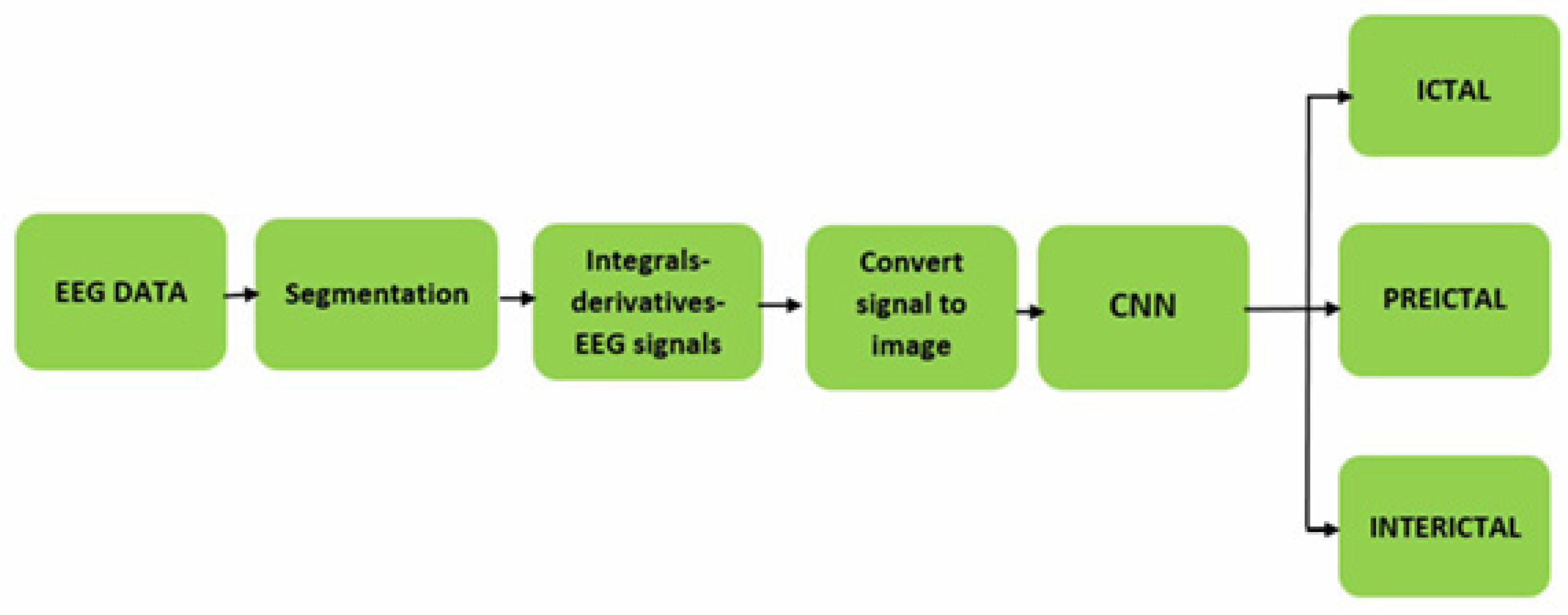
Figure 2.
Block diagram of the proposed feedback method.
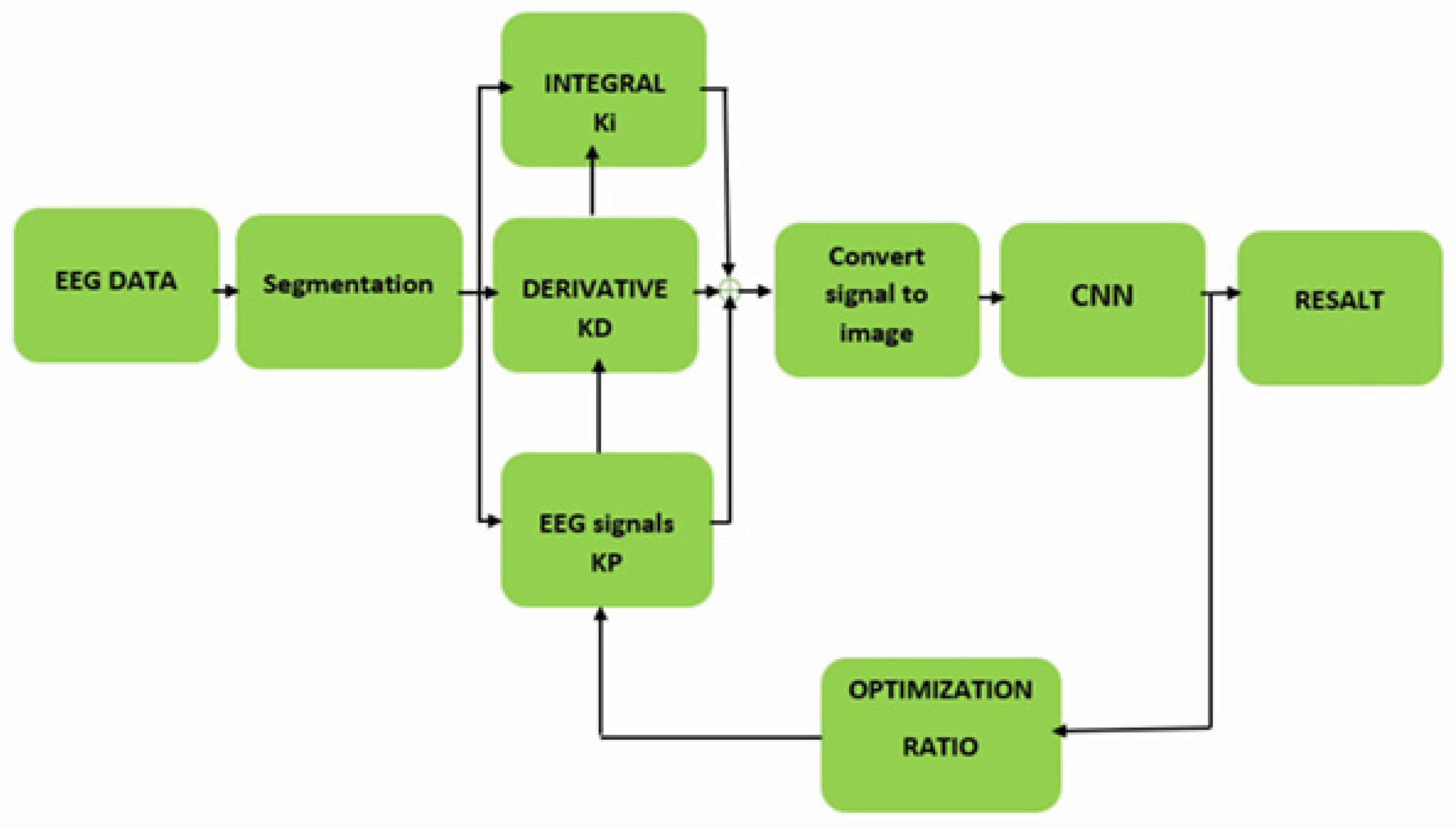
Figure 8.
Convolutional neural network configuration.
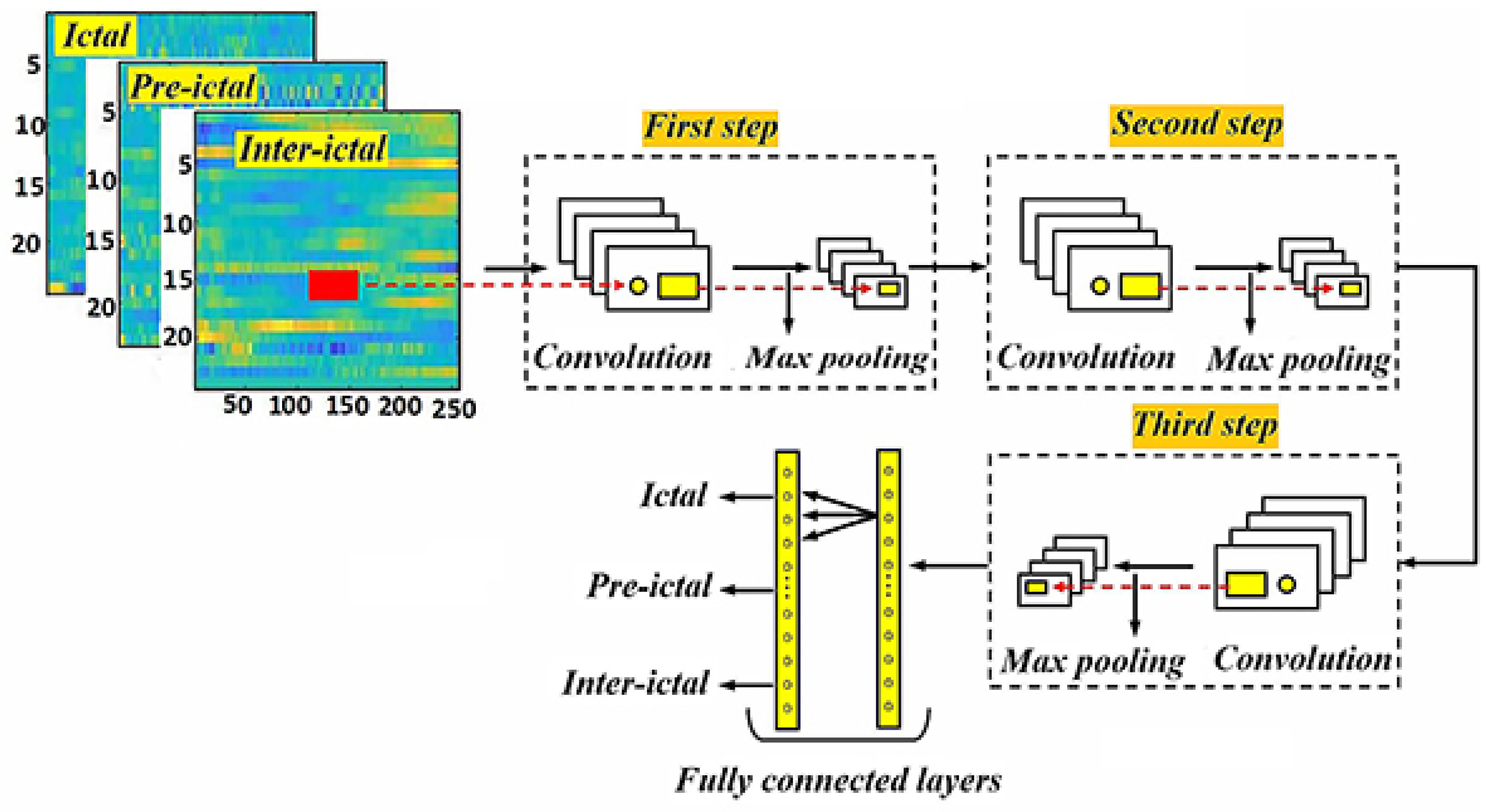
Figure 9.
Illustrates the process of testing and training the convolutional neural network.
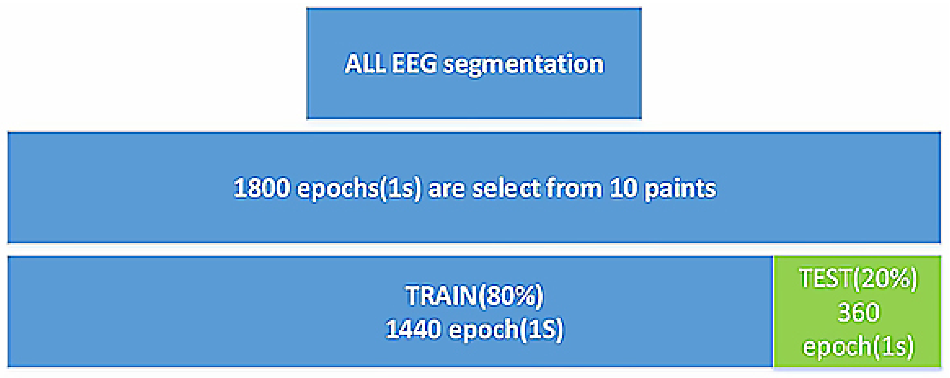
Figure 10.
Image generated by applying a hybrid function to ICTAL-INTERICTAL-PRE-ICTAL brain signals.
Figure 10.
Image generated by applying a hybrid function to ICTAL-INTERICTAL-PRE-ICTAL brain signals.
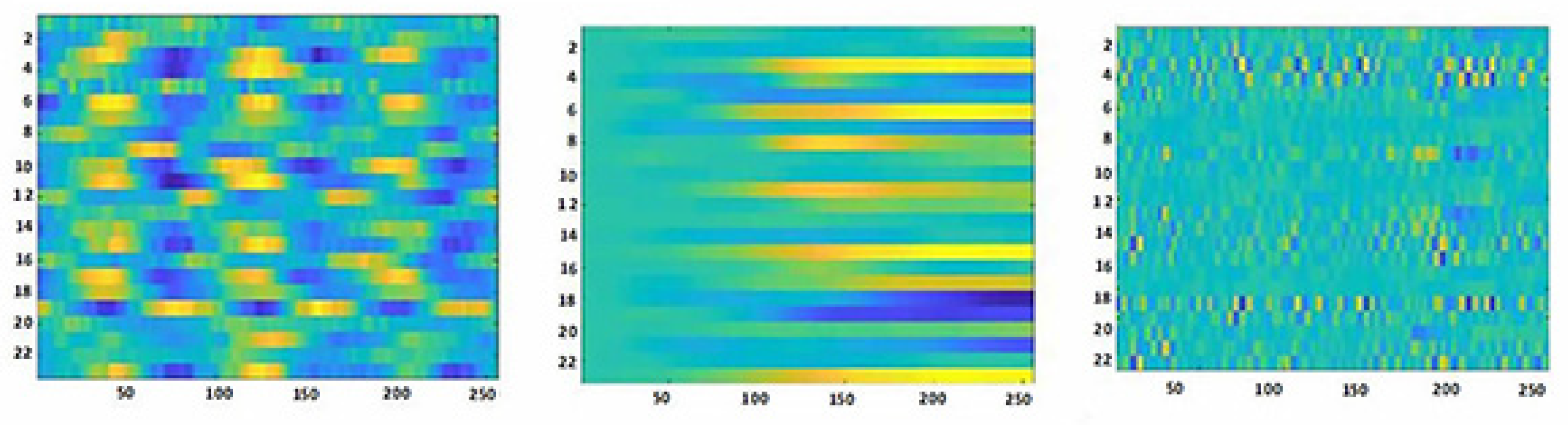

Table 1.
Characteristics of each convolutional neural network used in the test.
| Parameter | Search Space | Optimal Value |
| Optimizer | RMSProp, Adam, Sgd, Adamax, Steplr, Cycliclr | Sgd |
| Cost function | MSE, Cross-entropy | Cross-entropy |
| Dropout rate | 0,0.2,0.3,0.4,0.5 | 0.2 |
| Batch Size | 4,8,10,16,32,64,100 | 4 |
| Learning rate | 0.01,0.001,0.0001 | 0.0001 |
| Momentum and Gamma Parameters | 0.6,0.7,0.8,0.9 | 0.9 |
| Decay Rate of the Weights | 2, 3, 4 , 5 , 6 | 5 |
| Activation function after the BN Layer | Leaky-Relu , Sigmoid , Relu , Linear | Relu |
| Activation function in the first FC Layer | Leaky-Relu , Sigmoid , Relu , Linear | Relu |
| Activation function in the Last Layer | Softmax, Sigmoid | Softmax |
Table 2.
Dimensions of input and output images for each convolutional neural network used in the study.
Table 2.
Dimensions of input and output images for each convolutional neural network used in the study.
| Convolutional network architecture | Filter dimensions | Input image dimensions | Dimensions of the output image of the convolutional floor | Dimensions of Max Pauling floor output image | Number and dimensions of the output image |
| First part | 3×3 | 64×64 | 64×64 | 32×32 | 8@(32×32) |
| second part | 3×3 | 32×32 | 32×32 | 16×16 | 16@(16×16) |
| third part | 3×3 | 16×16 | 8×8 | 8×8 | 32@(8×8) |
Table 3.
Test results of conventional method and the effects of KP, Ki, and KD coefficients on data obtained from the CHB-MIT database.
Table 3.
Test results of conventional method and the effects of KP, Ki, and KD coefficients on data obtained from the CHB-MIT database.
|
Patient ID |
conventional method | basic method KP=0.5,KI=0.5,KD=5 | basic method KP=0,KI=0,KD=5 | basic method KP=KD=0,KI=10 |
||||||||
| acc | sen | spe | acc | sen | spe | acc | sen | spe | acc | acc | acc | |
| 1 | 0.611 | 0.781 | 0.720 | 0.8650 | 0.7738 | 0.8539 | 0.5833 | 0.9184 | 0.2333 | 0.6465 | 0.8387 | 0.5581 |
| 2 | 0.682 | 0.697 | 0.690 | 0.8565 | 0.7674 | 0.8621 | 0.6204 | 0.8889 | 0.3929 | 0.6162 | 0.7143 | 0.5641 |
| 3 | 0.656 | 0.660 | 0.658 | 0.7037 | 0.6239 | 0.7596 | 0.5463 | 0.8333 | 0.1724 | 0.6667 | 0.6458 | 0.7500 |
| 4 | 0.642 | 0.687 | 0.666 | 0.8608 | 0.8608 | 0.8132 | 0.5048 | 0.5345 | 0.4750 | 0.4921 | 0.4412 | 0.5625 |
| 5 | 0.600 | 0.645 | 0.623 | 0.8481 | 0.7778 | 0.8352 | 0.5714 | 0.6364 | 0.6389 | 0.5556 | 0.4999 | 0.7619 |
| 6 | 0.595 | 0.632 | 0.615 | 0.8312 | 0.7529 | 0.8242 | 0.5048 | 0.5345 | 0.4750 | 0.5873 | 0.4865 | 0.8542 |
| 7 | 0.620 | 0.666 | 0.643 | 0.8186 | 0.7294 | 0.7912 | 0.5349 | 0.7143 | 0.4717 | 0.5476 | 0.4881 | 0.8810 |
| 8 | 0.684 | 0.707 | 0.696 | 0.7829 | 0.7447 | 0.8077 | 0.5581 | 0.7547 | 0.4902 | 0.6984 | 0.5857 | 0.8667 |
| 9 | 0.642 | 0.625 | 0.633 | 0.8519 | 0.7660 | 0.9189 | 0.4806 | 0.7143 | 0.3922 | 0.6190 | 0.5181 | 0.8571 |
| 10 | 0.652 | 0.641 | 0.646 | 0.6952 | 0.5435 | 0.7500 | 0.5079 | 0.6418 | 0.5000 | 0.5079 | 0.6667 | 0.5714 |
| 11 | 0.657 | 0.649 | 0.653 | 0.8083 | 0.7334 | 0.8333 | 0.6566 | 0.7500 | 0.6154 | 0.6977 | 0.6744 | 0.6780 |
| 12 | 0.663 | 0.660 | 0.661 | 0.7847 | 0.7170 | 0.7963 | 0.7172 | 0.7381 | 0.6944 | 0.6883 | 0.5957 | 0.6939 |
| 13 | 0.645 | 0.628 | 0.636 | 0.8186 | 0.7619 | 0.7826 | 0.6162 | 0.7143 | 0.5641 | 0.7172 | 0.7381 | 0.6944 |
| 14 | 0.653 | 0.643 | 0.648 | 0.7132 | 0.8000 | 0.6905 | 0.7048 | 0.6739 | 0.7941 | 0.6667 | 0.6458 | 0.7500 |
| 15 | 0.636 | 0.615 | 0.625 | 0.7265 | 0.6465 | 0.7907 | 0.6970 | 0.7200 | 0.6452 | 0.7048 | 0.6739 | 0.7941 |
| 16 | 0.632 | 0.609 | 0.620 | 0.7847 | 0.7170 | 0.7963 | 0.4952 | 0.5818 | 0.5750 | 0.6286 | 0.5273 | 0.7317 |
Table 4.
Test results of the effect of the KD coefficient on the information downloaded from the CHB-MIT database of patient No. 08.
Table 4.
Test results of the effect of the KD coefficient on the information downloaded from the CHB-MIT database of patient No. 08.
| patient No. 08 | basic method KP=0.5,KI=0.2 | basic method KP=0.3,KI=0.3 | basic method KP=0.3,KI=0.5 | basic method KP=0.3,KI=0.6 | ||||||||
| %acc | %sen | %spe | %acc | %sen | %spe | %acc | %sen | %spe | %acc | %sen | %spe | |
| KD=0.1 | 0.8608 | 0.8235 | 0.8161 | 0.8734 | 0.7907 | 0.8824 | 0.8734 | 0.8118 | 0.8588 | 0.8945 | 0.8608 | 0.8506 |
| KD=0.2 | 0.8608 | 0.7952 | 0.8333 | 0.9072 | 0.8391 | 0.9136 | 0.8228 | 0.7556 | 0.8111 | 0.9156 | 0.8750 | 0.8851 |
| KD=0.3 | 0.8734 | 0.8000 | 0.8636 | 0.8861 | 0.8295 | 0.8941 | 0.8861 | 0.8391 | 0.8706 | 0.8523 | 0.7727 | 0.8636 |
| KD=0.4 | 0.8439 | 0.7294 | 0.8539 | 0.8861 | 0.8276 | 0.8824 | 0.8887 | 0.8395 | 0.8750 | 0.9072 | 0.8537 | 0.8953 |
| KD=0.5 | 0.9072 | 0.8571 | 0.8929 | 0.9072 | 0.8675 | 0.8824 | 0.8903 | 0.8452 | 0.8706 | 0.8861 | 0.8395 | 0.8506 |
| KD=0.6 | 0.8903 | 0.8140 | 0.8996 | 0.8439 | 0.7447 | 0.8721 | 0.8439 | 0.7391 | 0.8721 | 0.8819 | 0.8421 | 0.8352 |
| KD=0.7 | 0.8481 | 0.7831 | 0.8222 | 0.8734 | 0.8049 | 0.8539 | 0.8891 | 0.7791 | 0.9176 | 0.8692 | 0.8353 | 0.8576 |
| KD=0.8 | 0.8987 | 0.8022 | 0.9286 | 0.8861 | 0.8395 | 0.8506 | 0.8945 | 0.8214 | 0.8941 | 0.8945 | 0.8434 | 0.8736 |
| KD=0.9 | 0.8776 | 0.8415 | 0.8409 | 0.8734 | 0.7955 | 0.8824 | 0.8819 | 0.8375 | 0.8409 | 0.8987 | 0.8391 | 0.8902 |
| KD=1.00 | 0.8945 | 0.8642 | 0.8506 | 0.8819 | 0.8313 | 0.8506 | 0.8776 | 0.8313 | 0.8636 | 0.8819 | 0.8333 | 0.8953 |
Table 5.
Test results of the effect of the Ki coefficient on the information downloaded from the CHB-MIT database of patient No. 08.
Table 5.
Test results of the effect of the Ki coefficient on the information downloaded from the CHB-MIT database of patient No. 08.
| patient No. 08 | basic method KP=0.4,KD=0.9 | basic method KP=0.5,KD=0.9 | basic method KP=0.6,KD=0.9 | basic method KP=0.7,KD=0.9 |
||||||||
| %acc | %sen | %spe | %acc | %sen | %spe | %acc | %sen | %spe | %acc | %sen | %spe | |
| Ki=0.1 | 0.8565 | 0.8721 | 0.8172 | 0.8608 | 0.8608 | 0.8132 | 0.8608 | 0.7955 | 0.8571 | 0.8987 | 0.8919 | 0.8352 |
| Ki=0.2 | 0.8776 | 0.8642 | 0.8391 | 0.9114 | 0.8690 | 0.9059 | 0.8565 | 0.7792 | 0.8211 | 0.8734 | 0.8424 | 0.8523 |
| Ki=0.3 | 0.8565 | 0.8101 | 0.8111 | 0.8603 | 0.8118 | 0.8363 | 0.8692 | 0.8272 | 0.8352 | 0.9030 | 0.8452 | 0.9048 |
| Ki=0.4 | 0.8903 | 0.8500 | 0.8636 | 0.8481 | 0.7778 | 0.8352 | 0.8143 | 0.7284 | 0.7872 | 0.8650 | 0.8272 | 0.8409 |
| Ki=0.5 | 0.8312 | 0.7529 | 0.8242 | 0.8565 | 0.8023 | 0.8427 | 0.8776 | 0.8125 | 0.8556 | 0.8650 | 0.7976 | 0.8506 |
| Ki=0.6 | 0.8397 | 0.8705 | 0.8043 | 0.8565 | 0.8272 | 0.8111 | 0.8776 | 0.7976 | 0.8636 | 0.8903 | 0.8519 | 0.8523 |
| Ki=0.7 | 0.8397 | 0.7412 | 0.8352 | 0.8776 | 0.8333 | 0.8444 | 0.8776 | 0.8072 | 0.8652 | 0.8650 | 0.8140 | 0.8588 |
| Ki=0.8 | 0.8945 | 0.8353 | 0.9059 | 0.8692 | 0.8493 | 0.8105 | 0.8819 | 0.8500 | 0.8523 | 0.8945 | 0.8659 | 0.8605 |
| Ki=0.9 | 0.8565 | 0.8068 | 0.8488 | 0.8481 | 0.7412 | 0.8539 | 0.8734 | 0.8171 | 0.8427 | 0.8987 | 0.8235 | 0.8953 |
| Ki=1.00 | 0.8186 | 0.7294 | 0.7912 | 0.8945 | 0.8395 | 0.8652 | 0.8608 | 0.7619 | 0.8556 | 0.8945 | 0.8642 | 0.8506 |
Table 6.
Results of identical and non-identical integration tests on the base method.
|
KP, Ki and KD coefficients |
Results of identical integration tests |
Results of non-identical integration tests | |||||
| %acc | %sen | %spe | %acc | %sen | %spe | ||
| 1 | basic method KP=0.3,Ki=0.1,KD=0.8 |
0.6694 | 0.7329 | 0.6620 | 0.5048 | 0.5345 | 0.4750 |
| 2 | basic method KP=0.3,Ki=0.8,KD=0.5 |
0.6148 | 0.7288 | 0.6000 | 0.5048 | 0.5345 | 0.4750 |
| 3 | basic method KP=0.3,Ki=0.8,KD=0.2 |
0.6889 | 0.6942 | 0.7500 | 0.5048 | 0.5345 | 0.4750 |
| 4 | basic method KP=0.3,Ki=0.4,KD=1 |
0.7037 | 0.6239 | 0.7596 | 0.5714 | 0.6364 | 0.6389 |
| 5 | basic method KP=0.2,Ki=0.8,KD=0.2 |
0.6704 | 0.6466 | 0.7027 | 0.4762 | 0.4800 | 0.5217 |
| 6 | basic method KP=0.3,Ki=0.8,KD=0.5 |
0.7000 | 0.6917 | 0.7624 | 0.5048 | 0.5345 | 0.4750 |
| 7 | basic method KP=0.2,Ki=0.7,KD=2 |
0.7037 | 0.6581 | 0.7670 | 0.5714 | 0.6364 | 0.6389 |
| 8 | basic method KP=0.7,Ki=0.2,KD=2 |
0.6926 | 0.6789 | 0.7156 | 0.8945 |
0.8642 |
0.9059 |
| 9 | basic method KP=Ki=0.1,KD=5 |
0.7000 | 0.6695 | 0.7596 | 0.5079 | 0.6418 | 0.5000 |
| 10 | basic method KP=Ki=0.1,KD=2 |
0.9114 | 0.8690 | 0.8506 |
0.5079 | 0.6418 | 0.5000 |
Table 7.
Comparison between the results of the proposed methods and the conventional method.
| Accuracy% | Accuracy% | ||
| case | method | non-uniform integration method | uniform integration method |
| 1 | conventional method | 47% | 50% |
| 2 | basic method | 89% | 91% |
| 3 | feedback method | 93% | 95% |
Table 8.
Comparison between the results of the proposed method and other methods.
| Case | Authors | Dataset | Accuracy% | Sensitivity% | Specificity% |
| 1 | Xiaoyan Wei et al, 2018.[19] | Department of Neurology-Xinjiang Medical University | 90 | 88.9 | 93.78 |
| 2 | M. Hosseini et al , 2017.[20] | the Center for Epilepsy | 93 | 94 | 94 |
| 3 | Mengni Zhou1 et al, 2018.[21] | The CHB-MIT | 91.1 | 83.6 | 85.1 |
| 4 | Zhang, S. et al , 2020.[25] | The CHB-MIT | 89.98 | 92.9 | 87.04 |
| 5 | Zuyi Yu · Weiwei Nie, 2018.[26] | the Center for Epilepsy at Freiburg University Hospital in Germany | - | 87.7 | - |
| 6 | Jana R., 2020.[27] | The CHB-MIT | 94.33 | 96 | 94.39 |
| 7 | S. Muhammad Usman, 2020.[28] | The CHB-MIT | - | 92.7 | 90.8 |
| 8 | Zuochen Wei, 2019.[30] | The CHB-MIT | 81.49 | 70.68 | 92.30 |
| 9 | S. Raghu 2020.[31] | The Temple University Hospital (TUH) | 88.3 | 88.4 | 84.1 |
| 10 | proposed method | The CHB-MIT | 97.1 | 97.5 | 96.3 |
Disclaimer/Publisher’s Note: The statements, opinions and data contained in all publications are solely those of the individual author(s) and contributor(s) and not of MDPI and/or the editor(s). MDPI and/or the editor(s) disclaim responsibility for any injury to people or property resulting from any ideas, methods, instructions or products referred to in the content. |
© 2023 by the authors. Licensee MDPI, Basel, Switzerland. This article is an open access article distributed under the terms and conditions of the Creative Commons Attribution (CC BY) license (http://creativecommons.org/licenses/by/4.0/).
Copyright: This open access article is published under a Creative Commons CC BY 4.0 license, which permit the free download, distribution, and reuse, provided that the author and preprint are cited in any reuse.


