Submitted:
21 July 2023
Posted:
25 July 2023
You are already at the latest version
Abstract
Electroencephalography (EEG) is essential for tracking brain activity and identifying seizure effects. However, epileptic behaviour can only be detected after a specialist has carefully analysed all EEG recordings along with a proper history of the patient. A skilled physician is required for the right epilepsy diagnosis and therapy. But most of the time, patients visit the clinician in the interictal stage with no proper history documented. Therefore, it was essential to the automatic prediction of stages of seizure. K nearest neighbours (KNN) and random forest (RF) models using raw EEG signals, preictal, ictal, postictal, and interictal stages were identified in this study. The possibility of these characteristics is explored by examining how well time-domain signals work in the prediction of epileptic stages using intracranial EEG datasets from Freiburg Hospital (FH), Children's Hospital Boston-Massachusetts Institute of Technology (CHB-MIT), and Temple University Hospital (TUHEEG). To test the viability of this approach, two different types of simulations were carried out on three binary classifications (interictal vs. preictal, interictal vs. ictal, preictal vs. postictal, and interictal vs. postictal), and one four-class problem (interictal vs. preictal vs. ictal vs. postictal) was performed for each model. The average accuracy when using time-domain signals in the FH database was 90.5% and 75.0%; CHB-MIT was 92.87% and 75.9%; and TUHEEG was 94.46% and 76.8%, respectively, for the KNN and RF models.
Keywords:
FH
; RF
; KNN
; CHB-MIT
; TUHEEG
; EEG
; Epilepsy
; Seizure stages
1. Introduction
A brain disorder called epilepsy is characterised by recurrent seizures brought on by erratically discharged electrical currents in the brain. Epilepsy is a chronic condition brought on by excessive electrical discharge in the brain, which results in unconsciousness and other uncontrollable behavioural changes [1,2]. Three-fourths of the 80% of epileptic patients in low- and middle-income countries experience either a treatment gap or a lack of anti-seizure medications. Because of this, epileptic events can happen at any time and with any frequency, which makes diagnosis and treatment challenging. Pre-ictal, ictal, post-ictal, and inter-ictal are the four stages of a seizure. Pre-ictal is just before the occurrence of an epileptic seizure; Ictal is the onset period; post-ictal is just after the onset up to 10 minutes; and inter-ictal is after around 10 minutes of onset and lasts till the next occurrence of a seizure. Figure 1 depicts all four stages of seizure. The pre-ictal stage usually involves dizziness, headache, and nausea and is followed by the stage of intense electrical activity in the brain called the ictal region. Then comes the post-ictal region, where the patient returns to baseline conditions along with symptoms like disorientation, drowsiness, and headache.
The advent of machine learning and their increasing popularity in healthcare applications make it possible to classify majorly a) seizure-free and b) different types of seizures, but it’s done in the ictal period, and having a high-frequency EEG signal with spikes makes classification a little simpler. A good amount of research work is available in the Ictal stage but not in the pre-Ictal and Inter-Ictal stages, and very little focus is placed on the detection of seizure types in different stages.
Here, different studies present in the literature based on stage detection like ictal, pre-ictal, interictal, post-ictal, sleep stage, and mental state have been focused. In [3,4], the epileptic episode in EEG signals was detected automatically using a least squares support vector machine classifier with a radial basis function kernel. Here, normal stage, ictal stage, and inter-ictal stage are distinguished from the recorded EEG signal. The authors have indicated a wide scope for this method if the investigations can be done with real-time data and a large dataset collected via a multi-centre clinical trial. Whereas autonomously generalised retrospective and patient-specific hybrid models have been carried out in [5,6,7]. These studies used Convolutional Neural Networks(CNN) and long short-term memory(LSTM) as classifier. To better categorise ictal, interictal, and preictal segments for each patient and make it suitable for real-time, the model automatically creates customizable characteristics. This work demonstrates that the accuracy of seizure detection can be greatly increased by combining CNNs and LSTMs, incorporating spatial and temporal context, and time-frequency domain information. On the other side, unlike most of the existing works focusing on seizure data or a single-variate method, this paper introduces a multi-variate method to characterise sensor-level brain functional connectivity from interictal EEG data to identify patients with generalised epilepsy. A total of nine connectivity features based on five different measures in time, frequency, and time-frequency domains have been tested. The solution has been validated by the K-Nearest Neighbour algorithm, classifying an epilepsy group (EG) vs. a healthy control (HC), and subsequently, with another cohort of patients characterised by non-epileptic attacks (NEAD), a psychogenic type of disorder was tried out [8,9].
Entropy-based methods [10,11] are widely used for the automated detection of seizures from EEG signals due to the nonlinear and chaotic nature of these signals. Two recently introduced entropy features, multiscale dispersion entropy (MDE) and refined composite multiscale dispersion entropy (RCMDE), are used for the detection of seizures. The ability of MDE and RCMDE to discriminate the normal EEGs of healthy subjects from the interictal (in between seizures) and ictal (during seizures) EEGs of epilepsy patients Two more parameters are investigated, namely, the number of classes c and embedding dimension m of MDE and RCMDE that provide the best performance for seizure detection. For this purpose, the MDE and RCMDE values are estimated from normal, interictal, and ictal EEG signals, and significant features are fed to a support vector machine (SVM) classifier. Where the sleep stage classification from single-channel EEG was tried using the statistical features in the time domain, the structural graph similarity and the K-means were combined to identify six sleep stages. This method extracts features efficiently without pre-processing the signal [12,13,14]. In [15,16,17], the feasibility of a passive brain-computer interface that uses electroencephalography to monitor changes in mental state on a single-trial basis and the frontal and central electrodes for fatigue detection, posterior alpha band and frontal beta band activity for frustration detection, and posterior alpha band activity for attention detection for feature extraction is discussed. Where classification against low levels of supervised training using time-frequency subbands until the sixth level using the dual-tree complex wavelet transform method is carried out in [18]. The feature extraction uses energy, standard deviation, root-mean-square, Shannon entropy, mean values, and maximum peaks, and these feature sets are passed through a general regression neural network (GRNN) for classification with a K-fold cross validation scheme under varying train-to-test ratios.
Most of such analysis is carried out with non-invasive EEG signal recording during clinical intervention. However, the information of patients who underwent invasive VEM was retrospectively examined [19,20,21]. It included at least one EIS and one SHS that happened during VEM, and the area of the brain where the EIS were evoked was removed. According to the classification used by Engel and the International League Against Epilepsy (ILAE), seizure outcome was assessed at three follow-up (FU) visits after surgery—one at one year, one at two years, and one at the last FU that was still possible.
In order to distinguish between a patient's three stages of "normal," "pre-ictal," and "ictal," Acharya et al. [22,23,24] used an ensemble of seven distinct classifiers, including the Fuzzy Surgeon Classifier (FSC), SVM, KNN, Probabilistic Neural Network, GMM, decision tree, and Nave Bayes. Overall precision is 98.1%. Using the processed data containing seven features, including entropy, RMS, skewness, and variance, [25,26] also employed various classifiers, including a logistic classifier, an uncorrelated normal density-based classifier (UDC), a polynomial classifier, a KNN, a PARZEN, a SVM, and a decision tree. They stated that the patient was being diagnosed with a "generalised seizure," which refers to a seizure that affects the entire brain without prior knowledge of the seizure focal spots. Optimal sample allocation methodology, a statistical sampling strategy, was proposed by Mursalin et al. [27], and they developed a feature selection algorithm to reduce the features. The combination of four classifiers—SVM, KNN, NB, Logistic Model Trees (LMT), and Random Forest—was used for the analysis.
Four classifiers, including SVM, KNN, random forest, and Adaboost, were utilised by Rand and Sriram [28] on a high-dimensional dataset created from 28 features. Their findings demonstrate that the SVM outperforms the cubic kernel. Using the dataset generated by 10-time and frequency characteristics, [28] employed SVM and random forests. A random forest classifier performs better than an SVM-based detector. Using four machine learning classifiers, including ANN, KNN, SVM, and random forest, on two well-known datasets—Freiburg and CHB-MIT—[29] classified the three distinct seizure states of "pre-ictal," "ictal," and "inter-ictal" seizures with 100% accuracy. For identifying the EEG signals, [30,31] suggested an automated approach employing iterative filtering and random forests. The classification accuracy of this work was 99.5% for the A against E subsets on the BONN dataset (A-E), 96% for the D versus E subsets, and 98.4% for the ABCD versus E classes of EEG signals. KNN is used to distinguish between the "seizure" and "non-seizure" classes, and random forest is used to explore the significant channels, according to [32]. Here, the dimension reduction issue is also helped by the random forest. The key advantage of choosing appropriate channels is that it enables the provision of pertinent information from the selected channels and lowers the computational cost of a classifier as well. Nevertheless, the authors omitted crucial details from channel selection, such as locating the seizure's position on the brain's scalp. The fundamental criticism in [30,31,32] is that a large number of features causes the attribute size of the dataset to grow, which negatively affects accuracy and calculation time.
From the literature, it is noted that automatic seizure detection plays a vital role in epilepsy treatment. Many studies have explained the role of machines and deep learning models in seizure diagnostics. To protect epileptic patients from sudden falls or understand their condition, it is important to detect and predict the stage of a seizure. In the recent past, few studies focused on seizure stage prediction, but classification of all stages with raw EEG data was not considered for most of the experiments.
2. Materials and Methods
Machine learning algorithms can be trained to classify pre-ictal, ictal, post-ictal, and inter-ictal stages using various types of data, such as EEG recordings, clinical data, and other patient characteristics. In this research work, mainly EEG recordings of all four stages are used.
2.1. Dataset
In this section, the dataset used for stage prediction is discussed.
2.1.1. Freiburg Hospital dataset
One of the datasets utilised in this analysis was produced by the Epilepsy Centre at the University Hospital of Freiburg, Germany. This database includes intracranial EEG (iEEG) data obtained during invasive presurgical epilepsy monitoring from 21 individuals with medically intractable focal epilepsy. To record directly from focal areas and to achieve a high signal-to-noise ratio with fewer artefacts, intracranial grid, strip, and depth electrodes were used. The EEG data were recorded using a 16-bit analog-to-digital converter and a 128-channel Neurofile NT digitally recorded EEG system with a sampling rate of 256 Hz (patient 12's data were sampled at 511 Hz but downsampled to 256 Hz). The collection includes 87 seizure recordings from 21 patients who each experienced 2–5 seizures over the course of the investigation. Six contacts were chosen for each patient in this database following a visual evaluation of the iEEG data by skilled epileptologists: three contacts in close proximity to the epileptic centre (epileptogenic zone) and three contacts in distant areas involved in seizure spread and propagation. With 13 women and 8 males, the subjects' ages ranged from 10 to 50. Each of the three forms of seizures—simple partial (SP), complex partial (CP), and generalised tonic-clonic (GTC)—was experienced by at least two of the patients. Eight patients had the epileptic focus in the hippocampus; two patients had it in both the neocortical and hippocampus; and eleven patients had it there. The times of the seizures and epileptiform activities were documented by board-certified epileptologists at the Epilepsy Centre.
2.1.2. Children's Hospital Boston-M Institute of Technology dataset
An open-source EEG database from CHB-MIT was one of the datasets used in this investigation. Using scalp electrodes, recordings were made for 23 young people with epilepsy. 17 female participants in the study, whose ages ranged from 1.5 to 19 years, and 5 male participants, whose ages ranged from 3 to 22 years, participated. One child's age and biological preference were ignored. A week prior to data collection, all subjects were instructed to stop using any relevant medications. The dataset consists of 23 paediatric patients, 844 hours of continuous EEG recording, and 163 convulsions. The majority of the scalp EEG data is recorded using 22 electrodes at a sampling rate of 256 Hz. According to expert judgements, each seizure's start and end times are clearly marked, and each patient had a distinct number and length of seizures.Numerous segments were picked for these two open-source datasets in order to find preictal and interictal signals. From raw signals, experts can immediately determine the ictal state, which is when patients start having seizures. The interictal interval serves as a representation of the normal state in between two seizures. The shift from the interictal to the ictal periods is marked by the pre-ictal interval. In this study, raw recordings were divided into 1-s epochs using the moving-window method, and the CNN was then applied to each patient to analyse the differences. Predicting pre-ictal and inter-ictal stages is the fundamental goal of this effort..
2.1.3. Temple University Hospital EEG Dataset
In this case, the GNSZ seizure dataset is considered. Here, EEG recordings taken 100 seconds before the start time of onset for the pre-ictal period and 100 seconds after 10 minutes of the stop time of onset for the inter-ictal period are considered. In Table 1, the data collected for GNSZ seizure type from TUHEEG for Pre-ictal and Inter-ictal stages are presented.
2.2. Machine learning models
In this section two machine learning models, namely KNN and RF is described in details.
2.2.1. K Nearest Neighbor
A non-parametric, instance-based machine learning technique called K-Nearest Neighbours (KNN) is used to solve classification and regression prediction problems. KNN is primarily employed for categorization and predictive models in industry, though. Because it uses all the data for training while classifying and lacks a dedicated training phase, this technique is also known as a lazy learning algorithm. KNN model perform equally good for binary class as well as multi class classification. It is also very popular in seizure detection from EEG signals[[84]. The algorithm works by storing all available instances and classifying new instances based on a majority vote of their K nearest neighbors. Here, K is mostly square root of N, where N is the number of dimension. For each test instance, the distance between test instance and each row of training instance is calculated with any of the method namely: Minkowski, Euclidean or Manhattan. The formula used for calculating distance using Generalized Minkowski, Euclidean, and Manhattan is given by (1), (2) and (3) respectively.
where, N represents number of dimensions and p is an integer, Out of the three methods, distance calculation using Euclidean distance is commonly used.
Dmi(x,y) =( ∑i=1N |xi – yi |p)1/p
De(x,y) =( ∑i=1N (xi – yi)2)1/2
Dm(x,y) = ∑i=1N |xi – yi|
Here K, which determines the number of nearest neighbors to consider, has a significant impact on the performance of the KNN algorithm. A smaller value of K will result in a more complex and flexible decision boundary, but is also more susceptible to noise and outliers in the data. A larger value of K results in a smoother and less flexible decision boundary and is less susceptible to noise and outliers. In practice, the value of K is typically selected using cross-validation techniques to balance the trade-off between over fitting and under fitting. Let us consider a dataset size S x N, with S number of samples having C number of classes with N features in each class. 80% of randomly selected data with their respective class label is stored as train data and 20% is stored as test data in a separate folder. Each train and test data has N dimensional data. Euclidean distance (as shown in (2)) is used to calculate the distance between each test sample to all the train samples and a distance array with their corresponding classes i.e. 0.8S x 2 is generated. Where 1st column represents Euclidean distance and second column represents class. The table is sorted in ascending order based on distance value. The top K rows are selected. The test sample is predicted with the most frequently appeared class in top K rows.
For an example, in Figure. 1, shows two classes i.e. red triangles (indicated seizure class) and blue squares (indicated non seizure class) and green dot represents test sample. The smallest circle represents K=3 as the diameter of the circle is chosen such that 3 nearest samples of the test sample are accommodated. The dotted circle is for K=5, where 5 nearest samples are fitted. Here, for K=1 the nearest sample is red triangle i.e. seizure class so if K=1 is considered then the test sample is classified as seizure class, even in case of K=3, two red triangle and one blue square is closest. Therefore, it is classified as seizure class. But in case of K=5, its seen that out of 5 nearest neighbors Three belongs to non seizure class and two belongs to seizure class. Accordingly, it is classified as non seizure class, indicating that the selection of K is crucial.
One advantage of KNN is its simplicity and ease of implementation, making it a good choice for exploratory analyses or small-scale applications. Additionally, KNN can handle non-linear relationships between EEG signals and seizures, and it is less prone to over fitting compared to other machine learning algorithms.
2.2.2. Random Forest
RF is one of the most frequently used supervised machine learning technique for classification and regression problems. In case of classification, majority votes from the DTs are considered, and average value in case of regression. The ability to handle data sets with continuous variables, as in regression, and categorical variables, as in classification, is one of its most crucial qualities. RF is a robust algorithm that can handle noisy and high-dimensional data. However, it is also prone to over fitting if the trees are grown too deep. To mitigate this issue, techniques such as pruning or limiting the maximum depth of the trees are used. Additionally, RF can be computationally expensive if the number of trees is large, techniques requires like parallel processing or bagging to be used to speed up the computation. It is a type of ensemble algorithm, builds multiple DTs and aggregating their results to make a final prediction as depicted in Figure .2. Ensemble uses two types of techniques, they are bagging and boosting. RF uses bagging type, which is also known as Bootstrap Aggregation method. A random sample or random subset is selected via bagging from the complete data set. As a result, each model is created using the samples (Bootstrap Samples) that the Original Data gave, with a replacement process known as row sampling. Bootstrap refers to this stage of row sampling with replacement. Currently, each model is trained separately, producing results. After merging the outputs of all the models, the final decision is made based on a majority vote. Aggregation is the process of aggregating all the results and producing a result based on a majority vote. In Figure 2, It is observed that bootstrap 1, 2 and N has randomly considered samples from original data, therefore the samples are not unique. The DT models trained independently using bootstrapped samples. Based on the decision by majority trees, class is allotted to the sample under test.
In DT model, there are three nodes. They are a) root node, which is feature based and from where samples start dividing, b) decision node which are the nodes after splitting a root node, and c) leaf node are the last nodes where further splitting not possible. To select a feature for root node to split further, it is to know purity of the split. The purity of sub split is each leaf node has possibility of one class not multiple classes. To select the feature to take as root node the impurity of the dataset is calculated using Gini index as shown in (4) for multi classes and Gini index shown in (5) for binary class data.
where, P+ and P- is probability of positive or negative class, and Pi is probability of ith class.
Gini Index = 1 - ∑i=1N (Pi)2 for N classes
= 1- [ (P+)2 + (P-)2 ] for binary class
The algorithm finds the Gini index of all the possible splits and root node feature is selected which gives lowest Gini index. Lowest Gini index indicates low impurity. Apart from Gini index, “Entropy” also used to measure the impurity of the split. (6) represents the mathematical formula of Entropy.
where S represents sample.
E(S) = - ( P (+) log P (+) ) – (P (-)log P (-))
Gini index is computationally efficient and fast compare to Entropy and commonly used for impurity calculation and selection of feature for each root node in DT. To enhance the prediction power or to speed up prediction process, two ways hyper parameters are used in RF. Prediction power is increased using selection of proper number of DTs known as n_estimators, maximum attributes considered for splitting a node known as max_features, selection of minimum number of leafs and maximum number of leaf node in DT i.e. mini_sample_leaf and max_leaf_nodes. To increase the speed of the prediction, the number of processor allowed to use is pre fixed, randomness of the samples are controlled and one third of the samples are not used during training, but used for evaluate the model performance. This one third samples are termed as out of bag (OOB) samples.
3. Results
In this experimentation, three binary class classification and one four class classification is considered for three datasets, i.e. FH, CHB-MIT and TUHEEG.
3.1. Result obtained for Feiburg Hospital Dataset
Table 3 describes the performance of CNN model in the FH database.
Total 13 patients(PAT) results are noted and the average of all the patients for three binary classes i.e. preictal versus interictal, ictal versus interictal and postictal versus interictal are 79.7%, 93.69%, and 83.85% respectively. Out of 13 patients, model shows satisfactory performance for nine patients, but patient numbers 5,14,19,20 shows 60%, 25%, 25% and 60% accuracy for preictal versus interictal classification. However, patient numbers 1, 3,6,15,18,21 shows 100% accuracy for all the three binary classification method. Table 3, Table 4 and Table 5 shows part wise accuracy for FH dataset and CHB-MIT dataset and two class classification accuracy for TUHEEG dataset respectively.
3.2. Result obtained for CHB-MIT Dataset
Table 4 describes the performance of CNN model in the CHB-MIT database. Total 13 patients(PAT) results are noted and the average of all the patients for three binary classes i.e. preictal versus interictal, ictal versus interictal and postictal versus interictal are 84.4%, 93.01%, and 85.38% respectively. Out of 13 patients, model shows satisfactory performance for nine patients, but patient numbers 2,9,10,14 shows 33.33%, 50%, 66.67% and 60% accuracy for preictal versus interictal classification. However, patient numbers 1, 19,23 shows 100% accuracy for all the three binary classification method.
3.3. Result obtained for TUHEEG Dataset
Table 5 reports the performance of CNN model in the TUHEEG database. Total 18 patients informations are collected. The number of events collected for preictal, ictal, postictal, and interictal are 51,51, 51 and 44 respectively. The total number of events for each binary classification is shown in Table 5. It is noted that compare to preictal versus interictal and postictal versus interictal classification, ictal versus interictal shows the best performace in both the models. Here, KNN shows 96.38% and RF shows 91.57%. The seizure affect during preictal and postictal stage is less compare to ictal stage. The accuracies in that classes are little low.
The mathematical formula for calculating accuracy, precision, sensitivity, F1 score, and each class accuracy is shown in (4), (5), (6), (7) and (8) respectively.
where TP is True Positive, TN is True Negative.
Over all accuracy = (TP +TN)/ (TP+TN+FP+FN)
Precision = TP/(TP+FP)
Sensitivity = TP/(TP+FN)
F1 score = TP/(TP+ 0.5 x(FN+FP))
Class accuracy= TP/(TP+FN)
The Table 6, Table 7 and Table 8 describes accuracy, precision, sensitivity and F1 score of binary seizure stage prediction using CNN model of three datasets for preictal versus interictal, ictal versus interictal, and postictal versus interictal respectively. Whereas, Table 9 represents the train and test accuracies of three datasets for four class classification i.e., preictal versus ictal versus postictal versus interictal. For this experimentation, train –test ratio is considered as 80:20. Out of train data, 10% is used for validation.
4. Discussion
In this work number of seizure events considered from FH and CHB-MIT are 59 and 64 respectively. From each patient mentioned in Table 3 and Table 4, preictal, postictal, and interictal EEG signals are extracted. From TUHEEG dataset, 51 events considered for preictal, ictal and postictal and 44 events are considered for interictal stage. The total number of samples are shown in Table 1. Table 6, Table 7 and Table 8 shows accuracies of each stages for binary class classification i.e. preictal vs interictal, ictal vs interictal and postictal vs interictal using KNN and RF models, where K=1 and 50 numbers of trees are used respectively. The tables also include precision, sensitivity and F1 score of each stages. It is observed that 1)KNN model performed better than RF and also 2) prediction of each stage in binary classification is quite satisfactory. In binary classification interictal versus other three stages are considered , keeping in mind , most of the patients consult clinician in interictal stage. So it’s very important to train models to predict interictal stages accurately. Whereas, Table 9 describes four class classification using KNN and RF model. This table includes train and test accuracy of all the three datasets using both the models. It is noted that the train and test accuracy is comparable for both the models, indicating that data is not over fitted. In four class classification TUHEEG dataset with KNN model shows comparatively the best result i.e. 94.46% accuracy. All the three datasets also shows accuracy quite comparable, which validates the reliability of the models.
In future, RF can be modeled with different number of trees to increase the performance. Also other machine and deep learning models can be developed to predict stages and the best model can be adopted as diagnostic aid. Researchers also can experiment to find types of seizure in different stages.
5. Conclusions
Currently, a variety of conventional and cutting-edge technologies are generally used to assess epileptic activity in EEG recordings. A speedier diagnosis, ongoing monitoring, and a decrease in the overall cost of medical care are just a few benefits of automating this procedure. In this work, a very straightforward KNN and RF structures are used to avoiding the challenging feature extraction procedure. To verify the efficacy of the model, the Freiburg, CHB-MIT and TUHEEG datasets are examined. The average accuracy when using time-domain signals in the FH database was 90.5% and 75.0%; CHB-MIT was 92.87% and 75.9%; and TUHEEG was 94.46% and 76.8%, respectively, for the KNN and RF models. All three datasets are trained and tested at an 80:20 ratio. Epileptic EEG signals from all three datasets—pre-Ictal, ictal, postictal, and inter-Ictal stages—have been extracted. The KNN and RF models are used to predict preictal, ictal, postictal, and interictal stages.
Author Contributions
Conceptualization by all three authors; Introduction and literature review by Dr. Premila Manohar and Dr. Indira; methodology by all three authors;; modeling by Kusumika Krori Dutta ; validation, Dr. Premila Manohar and Dr. Indira K.; formal analysis, data collection, Kusumika Krori Dutta.; writing—original draft preparation, all three authore; writing—review and editing, all three authors.; visualization, Kusumika Krori Dutta.; supervision, Dr. Premila Manohar.; project administration, Dr. Indira K.; All authors have read and agreed to the published version of the manuscript.
Funding
This research received no external funding.
Data Availability Statement
FH EEG dataset is available @ https://epilepsy.uni-freiburg.de/freiburg-seizure-prediction-project/eeg-database. CHB-MIT dataset is available @ https://physionet.org/content/chbmit/1.0.0/ TUHEEG dataset is available https://isip.piconepress.com/projects/tuh_eeg/html/downloads.shtml.
Conflicts of Interest
The authors declare no conflict of interest. The funders had no role in the design of the study; in the collection, analyses, or interpretation of data; in the writing of the manuscript; or in the decision to publish the results.
References
- Thurman DJ, Beghi E, Begley CE, Berg AT, Buchhalter JR, Ding D, Hesdorfer DC, Hauser WA, Kazis L, Kobau R et al (2011) Standards for epidemiologic studies and surveillance of epilepsy. Epilepsia 2011, 52, 2–26. [CrossRef]
- KK.Dutta. Epilepsy is a curse: Myth or Reality An article published by InnoHEALTH magazine digital team, , 2020. https://innohealthmagazine.com/2020/issues/epilepsy-is-a-curse-myth-or-reality/. 19 October.
- Manish Sharma, Ram Bilas Pachori, U. Rajendra Acharya “A new approach to characterize epileptic seizures using analytic time-frequency flexible wavelet transform and fractal dimension”, Elsevier, Pattern Recognition Letters 2017, 94, 172–179. [CrossRef]
- Ram Bilas Pachori, Shivnarayan Patidar, “Epileptic seizure classification in EEG signals using second-order difference plot of intrinsic mode functions”. Elsevier, Computer methods and programs in biomedicine 2014, 113, 494–502. [CrossRef] [PubMed]
- Hussain, Waqar, “ Epileptic seizure detection using 1 D-convolutional long short-term memory neural networks”. Applied Acoustics 2021, 177. [CrossRef]
- Tuncer, Türker, “Epilepsy attacks recognition based on 1D octal pattern, wavelet transform and EEG signals”, Multimedia Tools and Applications 2021. [CrossRef]
- Raghu, S. Sriraam, Natarajan Temel, Yasin Rao, Shyam Vasudeva Kubben, Pieter L. , EEG based multi-class seizure type classification using convolutional neural network and transfer learning, Neural Networks 2020, 124, 202–212. [Google Scholar] [CrossRef] [PubMed]
- Cao, Jun Grajcar, Kacper Shan, Xiaocai Zhao, Yifan Zou, Jiaru Chen, Liangyu Li, Zhiqing Grunewald, Richard Zis, Panagiotis De Marco, Matteo Unwin, Zoe Blackburn, Daniel Sarrigiannis, Ptolemaios G., Using interictal seizure-free EEG data to recognise patients with epilepsy based on machine learning of brain functional connectivity. Biomedical Signal Processing and Control 2021, 67. [CrossRef]
- KK Dutta, Premila Manohar, Indira K, Falak Naaz, Meenakshi Lakshminarayan, Shwethaa Rajagopalan, “Seven Epileptic Seizure Type Classification in Pre-Ictal, Ictal and Interictal Stages Using Machine Learning Techniques”, Advances in Machine Learning & Artificial Intelligence(AMLAI), Vol 4, Issue 1, 23, pp 1-10. 20 January. [CrossRef]
- Sukriti, “Automated detection of epileptic seizures using multiscale and refined composite multiscale dispersion entropy”. Chaos, Solitons and Fractals 2021, 146. [CrossRef]
- KK Dutta, Kavya V., Sunny Arokia Swamy, "Removal of Muscle Artifacts from EEG Based on Ensemble Empirical Mode Decomposition and classification of Seizure using Machine Learning Techniques", IEEE- International Conference on Inventive Computing and Informatics (ICICI 2017)23-24 Nov'17, IEEE Xplore Compliant - Part Number: CFP17L34-ART, ISBN: 978-1-5386-4031-9.
- Mohammed Diykh, Yan Li; Peng Wen “EEG Sleep stage classification based on Time domain features and structural graph similarity”. IEEE Transaction on neural systems and rehabilitation engineering 2016, 24, 1159–1168. [CrossRef] [PubMed]
- Abeg Kumar Jaiswal, Haider Banka “Local pattern transformation-based feature extraction techniques for classification of epileptic EEG signals”, 2017, 34, 81–92. Elsevier, Biomedical Signal Processing and Control 2017, 34, 81–92. [CrossRef]
- Rajeev Sharma, Ram Bilas Pachori,“Classification of epileptic seizures in EEG signals based on phase space representation of intrinsic mode function”, Elsevier, Expert Systems with Application 2015, 42, 1106–1117. [CrossRef]
- Andrew Myrden,Tom Chau, “A passive EEG-BCI for Single-Trail Detection of Changes in Mental State”, IEEE Transaction on neural systems and rehabilitation engineering, 2017, 25, 345–357. [CrossRef]
- Shivnarayan Patidar, Trilochan Panigrahi, “Detection of epileptic seizure using Kraskov entropy applied on tunable -Q wavelet transform of EEG signals”, Elsivier, Biomedical signal Processing and Control 2017, 34, 74–80. [CrossRef]
- Abhijit Bhattacharyya, Ram Bilas Pachori, “Tunable -Q wavelet Transform Based multiscale entropy measure for automated classification of epileptic EEG signals”, Applied Science Journal 2017, 385. [CrossRef]
- Piyush Swami, Tapan K. Gandhi, Bijaya K. Panigrahi, Manjari Tripathi, Sneh Anand, “A novel robust diagnostic model to detect seizures in electroencephalography”. Elsevier, Elsevier, Expert Systems with Application 2016, 56, 116–130. [CrossRef]
- Kämpfer, Christopher, “Predictive value of electrically induced seizures for postsurgical seizure outcome”, Clinical Neurophysiology 2020, 131. [CrossRef]
- Mingyang Li, Wanzhong Chen, Tao Zhang “Automatic epileptic EEG detection using DT-CWT-based non-linear features”, Elsivier, Biomedical signal Processing and Control 2017, 34, 114–125. [CrossRef]
- Zarei, Asghar, “Automatic seizure detection using orthogonal matching pursuit, discrete wavelet transform, and entropy based features of EEG signals”, Computers in Biology and Medicine 2021, 131. [CrossRef]
- Acharya UR, Molinari F, Sree SV, Chattopadhyay S, Ng K-H, Suri JS. Automated diagnosis of epileptic EEG using entropies. Biomed Sign Process Contr 2012, 7, 401–408. [CrossRef]
- Dr. Arun S, KK Dutta, book chapter titled," Application of Machine Learning techniques in Electroencephalography signals", chapter 3 of book titled," Brain & Behavior Computing", CRC press, (c) Taylor & Francis group, ISBN: 978-1-003-09288-9 (ebk), 21. 20 August.
- Muhammad Shoaib Farooq,* Aimen Zulfiqar, and Shamyla Riaz, Dinesh Bhati, “Epileptic Seizure Detection Using Machine Learning: Taxonomy, Opportunities, and Challenges”, Diagnostics (Basel). 2023, 13, 1058. [CrossRef]
- Fergus P, Hussain A, Hignett D, Al-Jumeily D, Abdel-Aziz K, Hamdan H. A machine learning system for automated whole-brain seizure detection. Appl Comput Inform 2016, 12, 70–89. [CrossRef]
- K Indira, KK Dutta, S Poornima, SA Swamy Bellary, book chapter titled “Deep Learning Methods for Data Science”, ch7 of book titled “Advanced Analytics and Deep Learning Models”, May2022, Publisher John Wiley & Sons, Inc. 149-179. [CrossRef]
- Mursalin M, Islam SS, Noman MK. Epileptic seizure classification using statistical sampling and a novel feature selection algorithm. arXiv arXiv:1902.09962, 2019.
- Raghu S, Sriraam N. Classifcation of focal and non-focal EEG signals using neighborhood component analysis and machine learning algorithms. Exp Syst Appl 2018, 113, 18–32. [CrossRef]
- Manzouri F, Heller S, Dümpelmann M, Woias P, Schulze-Bonhage, A. A comparison of machine learning classifers for energyefcient implementation of seizure detection. Front Syst Neurosci 2018, 12, 43.
- Alickovic E, Kevric J, Subasi A. Performance evaluation of empirical mode decomposition, discrete wavelet transform, and wavelet packed decomposition for automated epileptic seizure detection and prediction. Biomed Sign Process Contr 2018, 39, 94–102. [CrossRef]
- Tuncer, Turker, “Automated EEG signal classification using chaotic local binary pattern”, Expert Systems with Applications 2021, 182. [CrossRef]
- Sharma RR, Varshney P, Pachori RB, Vishvakarma SK (2018) Automated system for epileptic EEG detection using iterative fltering. IEEE Sens Lett 2018, 2, 1–4. [CrossRef]
- C. Shang and F. You, Data Analytics and Machine Learning for Smart Process Manufacturing: Recent Advances and Perspectives in the Big Data Era. Engineering, 2019, 5, 1010–1016. [CrossRef]
Figure 1.
KNN Model for three class system.
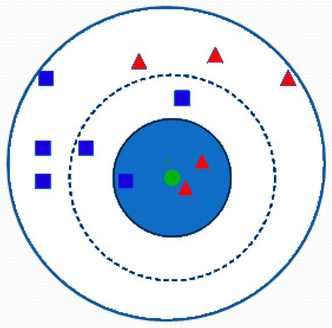
Figure 2.
Bagging method for random forest.
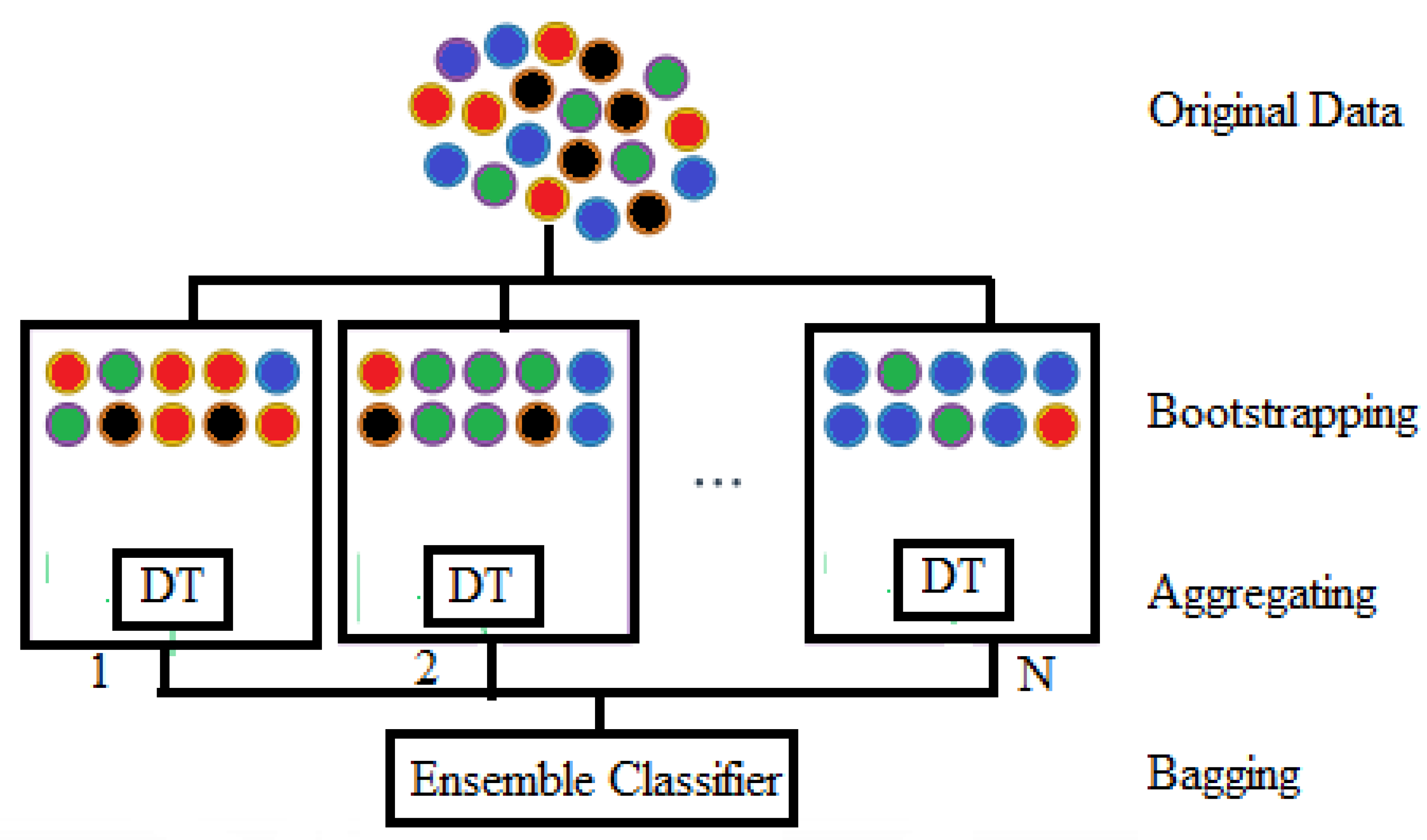

Table 1.
Data collection from TUHEEG.
| Pre-Ictalbreak//Samples NE | Ictal break//Samples NE | Post-Ictal break//Samples NE | Inter-Ictalbreak//Samples NE |
|---|---|---|---|
| 725600 51 | 733780 51 | 725600 51 | 737000 44 |
Table 3.
Seizure prediction results using FH iEEG dataset.
| Models | KNN | RF | ||||||
|---|---|---|---|---|---|---|---|---|
| Patients | No. of seizures | No. of Hours | Acc(%)break//Pre-ictal Vs Inter-ictal | Acc(%)break//Ictal Vs Inter-ictal | Acc(%)break//Post-ictal Vs Inter-ictal | Acc(%)break//Pre-ictal Vs Inter-ictal | Acc(%)break//Ictal Vs Inter-ictal | Acc(%)break//Post-ictal Vs Inter-ictal |
| PAT1 | 4 | 23.9 | 100 | 100 | 100 | 88.5 | 100 | 88.5 |
| PAT3 | 5 | 23.9 | 88.2 | 94.0 | 86.2 | 50.211 | 85.25 | 66.431 |
| PAT4 | 5 | 23.9 | 100 | 100 | 100 | 93.5 | 100 | 93.5 |
| PAT5 | 5 | 23.9 | 90.36 | 100 | 90.36 | 80.4 | 90.31 | 90.9 |
| PAT6 | 3 | 23.8 | 84.91 | 98.51 | 81.91 | 77.23 | 84.91 | 92.81 |
| PAT14 | 4 | 22.6 | 90.4 | 97.5 | 90.4 | 75.78 | 90.4 | 85.78 |
| PAT15 | 4 | 23.7 | 98.5 | 99.25 | 98.5 | 86.4 | 95.5 | 86.4 |
| PAT16 | 5 | 23.9 | 78.05 | 98.75 | 70.0 | 75.14 | 78.05 | 89.34 |
| PAT17 | 5 | 24 | 100 | 100 | 100 | 98.25 | 100 | 98.25 |
| PAT18 | 5 | 24.8 | 100 | 100 | 100 | 94.46 | 100 | 94.46 |
| PAT19 | 4 | 24.3 | 95.5 | 100 | 95.5 | 85.25 | 95.5 | 85.25 |
| PAT20 | 5 | 24.8 | 96.89 | 100 | 98.89 | 79.0 | 95.84 | 89.72 |
| PAT21 | 5 | 23.9 | 100 | 100 | 100 | 98.25 | 100 | 98.25 |
| TOTAL | 59 | 311.4 | 94.07 | 99.15 | 93.22 | 83.89 | 93.22 | 89.83 |
Table 4.
Seizure prediction results using CHB-MIT EEG dataset.
| Model | KNN | RF | ||||||
|---|---|---|---|---|---|---|---|---|
| Patients | No. of seizures | No. of Hours | Acc(%)break//Pre-ictal Vs Inter-ictal | Acc(%)break//ictal Vs Inter-ictal | Acc(%)break//Post-ictal Vs Inter-ictal | Acc(%)break//Pre-ictal Vs Inter-ictal | Acc(%)break//ictal Vs Inter-ictal | Acc(%)break//Post-ictal Vs Inter-ictal |
| PAT1 | 7 | 17 | 100 | 100 | 100 | 90.5 | 100 | 88.5 |
| PAT2 | 3 | 22.9 | 88.5 | 82 | 64.81 | 44.21 | 67.841 | 46.21 |
| PAT3 | 6 | 21.9 | 100 | 100 | 98.5 | 95.5 | 98.7 | 93.5 |
| PAT5 | 5 | 13 | 90.56 | 95 | 86.63 | 80.4 | 88.63 | 80.4 |
| PAT9 | 4 | 12.3 | 84.99 | 86.44 | 80.23 | 70.23 | 80.23 | 72.23 |
| PAT10 | 6 | 11.1 | 90.4 | 91.5 | 80.78 | 75.78 | 81.78 | 75.78 |
| PAT13 | 5 | 14 | 98.5 | 93 | 89.4 | 86.4 | 90.4 | 86.4 |
| PAT14 | 5 | 5 | 79.55 | 97 | 90.14 | 70.14 | 93.14 | 70.14 |
| PAT18 | 6 | 23 | 100 | 100 | 98.46 | 98.46 | 98.46 | 98.25 |
| PAT19 | 3 | 24.9 | 100 | 100 | 100 | 94.25 | 100 | 94.46 |
| PAT20 | 5 | 20 | 99.5 | 100 | 100 | 85.249 | 100 | 85.25 |
| PAT21 | 4 | 20.9 | 96.89 | 100 | 99.25 | 79.25 | 99.25 | 79.0 |
| PAT23 | 5 | 3 | 100 | 100 | 100 | 98 | 100 | 98.25 |
| TOTAL | 64 | 311.4 | 94.53 | 95.76 | 91.40 | 82.813 | 92.187 | 82.812 |
Table 5.
Seizure prediction results using TUHEEG dataset using binary classes.
| Models | KNN | RF | ||||
|---|---|---|---|---|---|---|
| Binary classes | Pre-ictal Vs Inter-ictal | ictal Vs Inter-ictal | Post-ictal Vs Inter-ictal | Pre-ictal Vs Inter-ictal | ictal Vs Inter-ictal | Post-ictal Vs Inter-ictal |
| Total events | 95 | 95 | 95 | 95 | 95 | 95 |
| Acuuracy in % | 91.43 | 96.385 | 93.66 | 88.17 | 91.57 | 86.315 |
Table 6.
Performance of prediction of preictal versus interictal.
| Model | KNN | RF | |||||
|---|---|---|---|---|---|---|---|
| Dataset | Matrics | Acc(%)break//Pre-Ictal | Acc(%)break// Inter-Ictal | Acc(%)break//Mean | Acc(%)break//Pre-Ictal | Acc(%)break// Inter-Ictal | Acc(%)break//Mean |
| FH | Accuracy | 94.91 | 93.22 | 94.07 | 83.05 | 84.74 | 83.89 |
| Precision | 93.33 | 94.83 | 94.08 | 84.48 | 83.33 | 83.91 | |
| Sensitivity | 94.91 | 93.22 | 94.07 | 83.05 | 84.74 | 83.89 | |
| F1 Score | 0.9412 | 0.9404 | 0.9407 | 0.837 | 0.8403 | 0.839 | |
| CHB-MIT | Accuracy | 92.18 | 96.87 | 94.53 | 78.12 | 87.5 | 82.813 |
| Precision | 96.72 | 92.53 | 94.63 | 86.20 | 80.0 | 83.103 | |
| Sensitivity | 92.18 | 96.87 | 94.53 | 78.12 | 87.5 | 82.813 | |
| F1 Score | 0.944 | 0.9466 | 0.9453 | 0.8197 | 0.835 | 0.8277 | |
| TUHEEG | Accuracy | 94.0 | 97.67 | 91.48 | 88.0 | 88.37 | 88.17 |
| Precision | 97.91 | 93.33 | 95.62 | 89.79 | 86.36 | 88.17 | |
| Sensitivity | 94.0 | 97.67 | 91.48 | 88.0 | 88.37 | 88.17 | |
| F1 Score | 0.9592 | 0.9545 | 0.9569 | 0.889 | 0.874 | 0.881 |
Table 7.
Performance of classification of each model for ictal vs interictal.
| Model | KNN | RF | |||||
|---|---|---|---|---|---|---|---|
| Dataset | Matrics | Acc(%)break//ictal | Acc(%)break// Inter-ictal | Acc(%)break//Mean | Acc(%)break//ictal | Acc(%)break// Inter-ictal | Acc(%)break//Mean |
| FH | Accuracy | 100.0 | 98.305 | 99.15 | 94.915 | 91.52 | 93.22 |
| Precision | 98.33 | 100 | 99.167 | 91.80 | 94.73 | 93.27 | |
| Sensitivity | 100.0 | 98.305 | 99.15 | 94.915 | 91.52 | 93.22 | |
| F1 Score | 0.9916 | 0.9915 | 0.9915 | 0.933 | 0.931 | 0.932 | |
| CHB-MIT | Accuracy | 94.44 | 96.87 | 95.76 | 90.625 | 93.75 | 92.187 |
| Precision | 96.23 | 95.38 | 95.81 | 93.54 | 90.90 | 92.23 | |
| Sensitivity | 94.44 | 96.87 | 95.76 | 90.625 | 93.75 | 92.187 | |
| F1 Score | 0.9533 | 0.961 | 0.9573 | 0.9206 | 0.9231 | 0.9219 | |
| TUHEEG | Accuracy | 97.436 | 95.45 | 96.385 | 92.31 | 90.91 | 91.57 |
| Precision | 95.0 | 97.67 | 96.337 | 90.0 | 93.02 | 91.51 | |
| Sensitivity | 97.436 | 95.45 | 96.385 | 92.31 | 90.91 | 91.57 | |
| F1 Score | 0.962 | 0.9655 | 0.9638 | 0.9114 | 0.9195 | 0.9155 |
Table 8.
Performance of prediction of postictal vs interictal.
| Model | KNN | RF | |||||
|---|---|---|---|---|---|---|---|
| Dataset | Matrics | Acc(%)break//Post-ictal | Acc(%)break// Inter-ictal | Acc(%)break//Mean | Acc(%)break//Post-ictal | Acc(%)break// Inter-ictal | Acc(%)break//Mean |
| FH | Accuracy | 91.525 | 94.915 | 93.22 | 88.13 | 91.52 | 89.83 |
| Precision | 94.73 | 91.803 | 93.27 | 91.23 | 88.52 | 89.88 | |
| Sensitivity | 91.525 | 94.915 | 93.22 | 88.13 | 91.52 | 89.83 | |
| F1 Score | 0.9310 | 0.933 | 0.9322 | 0.897 | 0.90 | 0.8983 | |
| CHB-MIT | Accuracy | 90.63 | 92.18 | 91.40 | 84.37 | 81.25 | 82.813 |
| Precision | 92.06 | 90.76 | 91.416 | 81.81 | 83.87 | 82.84 | |
| Sensitivity | 90.63 | 92.18 | 91.40 | 84.37 | 81.25 | 82.813 | |
| F1 Score | 0.913 | 0.9147 | 0.9141 | 0.831 | 0.825 | 0.8281 | |
| TUHEEG | Accuracy | 94.12 | 93.18 | 93.68 | 88.23 | 84.09 | 86.315 |
| Precision | 94.12 | 93.18 | 93.68 | 86.528 | 86.046 | 86.29 | |
| Sensitivity | 94.12 | 93.18 | 93.68 | 88.23 | 84.09 | 86.315 | |
| F1 Score | 0.9412 | 0.9318 | 0.9365 | 0.874 | 0.851 | 0.862 |
Table 9.
Seizure stage prediction results for preictal vs ictal vs postictal vs interictal.
| KNN | RF | |||
|---|---|---|---|---|
| Dataset | Acc(%)break//Train | Acc(%)break//Test | Acc(%)break//Train | Acc(%)break//Test |
| FH | 93.5 | 90.5 | 79.0 | 75.0 |
| CHB-MIT | 94.47 | 92.87 | 76.45 | 75.9 |
| TUHEEG | 98.66 | 94.46 | 77.8 | 76.8 |
Disclaimer/Publisher’s Note: The statements, opinions and data contained in all publications are solely those of the individual author(s) and contributor(s) and not of MDPI and/or the editor(s). MDPI and/or the editor(s) disclaim responsibility for any injury to people or property resulting from any ideas, methods, instructions or products referred to in the content. |
© 2023 by the authors. Licensee MDPI, Basel, Switzerland. This article is an open access article distributed under the terms and conditions of the Creative Commons Attribution (CC BY) license (https://creativecommons.org/licenses/by/4.0/).
Copyright: This open access article is published under a Creative Commons CC BY 4.0 license, which permit the free download, distribution, and reuse, provided that the author and preprint are cited in any reuse.


