Submitted:
17 June 2023
Posted:
19 June 2023
You are already at the latest version
Abstract
Epilepsy is a chronic neurological disorder characterized by abnormal electrical activity in the brain, often leading to recurrent seizures. With approximately 50 million people worldwide affected by epilepsy, there is a pressing need for efficient and accurate methods to detect and diagnose seizures. Electroencephalogram (EEG) signals, which record the brain’s electrical activity, have emerged as a valuable tool in detecting epilepsy and other neurological disorders. Traditionally, the process of analyzing EEG signals for seizure detection has relied on manual inspection by experts, which is time-consuming, labor-intensive, and susceptible to human error. To address these limitations, researchers have turned to machine learning and deep learning techniques to automate the seizure detection process. In this work, we propose a novel method for epileptic seizure detection, leveraging the power of 1-D Convolutional layers in combination with Bidirectional Long Short-Term Memory (LSTM) and Gated Recurrent Unit (GRU) and Average pooling Layer as a unit. The performance of the proposed model is verified on the Bonn dataset. Our proposed model offers significant advancements over existing approaches for the detection of epileptic seizures, particularly for 2, 3, 4, and 5-class classification tasks. To assess the robustness and generalizability of our proposed architecture, we employ 5-fold cross-validation. By dividing the dataset into five subsets and iteratively training and testing the model on different combinations of these subsets, we obtain robust performance measures, including accuracy, sensitivity, and specificity. We demonstrate the effectiveness of the proposed architecture in accurately detecting epileptic seizures from EEG signals by using EEG signals of varying lengths. The results indicate its potential as a reliable and efficient tool for automated seizure detection, paving the way for improved diagnosis and management of epilepsy.
Keywords:
Epilepsy
; seizure detection
; EEG signals
; LSTM
; GRU
; Convolutional Neural Networks
; Deep Learning
; Machine Learning
0. Introduction
Epilepsy is a prevalent chronic neural disorder caused by irregular electrical discharges in the brain, known as seizures. It causes recurrent seizures or convulsions. Seizures occur when there is abnormal electrical activity in the brain, leading to a temporary disruption in brain function. Epileptic seizures can vary in severity and duration and can cause a range of symptoms including loss of consciousness, convulsions, muscle spasms, confusion and sensory disturbances. Epilepsy is a neurological disorder that affects millions of people worldwide. About 50 million people worldwide are diagnosed with epilepsy [1]. Seizures are caused due to uncontrolled electrical discharges in a group of neurons in the brain which leads to disruption of the brain function [2]. More than 20% of epileptic patients experience one or more strokes in a month [3]. One of the critical challenges in managing epilepsy is the accurate and timely detection of seizures.
Electroencephalography(EEG) is a non-invasive method of recording brain activity widely used to detect epileptic seizures.The EEG records the voltage fluctuations resulting from the ionic flow of neurons in the brain, reflecting the brain’s bioelectric activity [4]. EEG signals have different stages based on their amplitude levels: preictal stage, postictal stage, ictal stage and interictal stage. The EEG signal before the onset of the seizure is called preictal. The starting state of seizure is classified as ictal. The stage after the ictal stage is called the postictal stage. The first occurring ictal stage is called as interictal stage [5]. Neurologists make inferences from the EEG signals by visual inspection of the EEG signals. It is a laborious and time-intensive process, often requiring skimming through hundreds of hours of EEG recordings. It is also highly dependent on the neurologist’s expertise in examining the EEG signals. Therefore, attempts have been made to automate the process of epileptic seizure detection from EEG signals using machine learning and deep learning. Many efforts have been made to use machine-learning techniques for the detection of epileptic seizures by extracting handwritten features in the time domain and frequency domain and often combining both these domains together. The performance of these models are limited to the ability of the experts handcrafting the features [6]. Achieving a high level of diagnostic accuracy by combining various feature extraction algorithms necessitates a considerable level of expertise in the field of machine learning [7,8]. These methods are not immune to the artifacts present in the EEG signals, and the accuracy of the detection of epileptic seizures can be affected greatly due to the presence of artifacts introduced due to muscle movements, eye blink, and white noise present in the environment. Biomedical signals like EEG signals are non-stationary, meaning that the statistical features change over time and for the same patient. The features extracted by deep learning models are proven to be more robust than the handcrafted features in several fields [9].
Deep learning methods can automate the detection of epileptic seizures from EEG signals by learning the relevant features from the raw signals, eliminating the need for manual feature engineering. Deep learning models, such as convolutional neural networks or recurrent neural networks (RNNs) for sequential data, are designed to automatically learn hierarchical representations of data through multiple layers of interconnected neurons.
However, standard recurrent neural networks are subject to the problem of vanishing gradients and exploding gradients [10,11]. To solve the problem of vanishing and exploding gradients, Long Short-Term Memory(LSTM) and Gated Recurrent Units(GRUs) can be used. There have been many recent advances in the detection of epileptic seizures from EEG signals. Most of the work in the field of detection involves two stages. The first stage involves extracting features: time-domain, frequency domain, or time-frequency domain[12]. Time-frequency methods such as Short-Time Fourier Transform [13], Hilbert Huang Transform [14], Discrete Wavelet Transform [15] and empirical mode decomposition[16] have been considered for the detection of epileptic seizures from EEG signals. The second stage involves feeding the hand-crafted features into the classifier. Researchers have made efforts toward seizure detection using machine learning and deep learning models. Ihsan Ullah et al.[17] proposed an ensemble of P-1D-CNN, i.e.pyramidal one-dimensional convolutional neural network models. The author has focused on ternary classification of epilepsy detection i.e. normal vs interictal vs ictal (AB vs. CD vs. E & A vs. C vs. E) and achieved an accuracy of approximately 99% on Bonn university dataset. Subhrajit Roy et al. [18] proposed a new architecture called Chrononet which consists of multiple 1-D convolution layer (stacked over each other with varying filter length) and stacked GRU in feed-forward manner. Ramy Hussein et al.[19] proposed a robust architecture for detecting epileptic seizures using Long Short-Term Memory (LSTM) network.
Thara D.K. et al. [20]. proposed a model for seizure detection as well as seizure prediction using stacked LSTM and Bidirectional LSTM. The accuracy obtained is 99% on the Bonn University dataset. Minyasan et al. [21] used neural network and fuzzy function with a combination of principal component analysis for seizure detection and achieved an accuracy of 97.64%.
Researchers in [22] applied Wavelet transform with wavelet denoising to get a sensitivity of 96.72% on mice EEG data. In [23], researchers have used deep neural networks trained with dropout for patient-specific epileptic seizure from EEG data. Researchers have also used deep belief networks (DBNs) to detect seizures in multi-channel EEG signal data[24]. Convolutional Neural Networks have also been used to detect the spikes in the EEG data [25]. CNN has been used to extract time-domain features from the intracranial EEG data from epileptic patients [28]. In [29], the authors have used multi-channel EEG wavelet spectra and 1-D convolutional neural networks to detect seizures in EEG signals.
In this work, a novel deep learning framework incorporating the use of units of 1D-CNN, Bidirectional LSTM and Average Pooling layer has been proposed for the classification of seizure and non-seizure EEG signals as well as multiclass classifications into different stages of seizures using the Bonn dataset. The proposed models have also been developed with Bidirectional GRUs instead of Bidirectional LSTMs and their performances have been compared. This work shows that both the models with Bi-LSTM and Bi-GRU give comparable results. The proposed work has shown to be effective in the detection of epileptic seizures n EEG signals in the presence of artifacts as well as in ideal conditions. It has been experimented on EEG signals of different durations to determine its effectiveness. A 5-fold cross-validation technique was employed to assess the performance of the model. The use of 5-fold cross-validation in the experiment offers several benefits, including robustness in evaluating the model’s performance, efficient utilization of data by partitioning it into subsets, and the ability to provide insights into the model’s generalization capabilities. The proposed work has been compared with the latest works in the field of seizure detection using EEG signals. We report that it has obtained significant improvements in the performance measures, namely accuracy, specificity, sensitivity and F1 score.
1. Materials and Methods
1.1. Dataset
The dataset used in this study is of EEG signals obtained from the Bonn University, Germany [30]. The dataset consists of 500 segments of EEG recordings divided evenly into five sets. These signals are recorded from a 128-channel amplifier using a 12-bit analog-to-digital converter. Each set has a total of 100 single-channel EEG signals with 4097 sample points per channel. Every signal has a duration of 23.6 seconds and a sampling frequency of 173.61 Hz. The dataset consists of five sets of EEG signals: A, B, C, D and E. Set A and set B are recorded from the scalp of five healthy subjects with their eyes open and closed, respectively. The set C, D and E are EEG signals collected from five epileptic patients. The set D consists of EEG signals recorded from the epileptogenic zone. Set C consists of EEG signals recorded from the opposite hemisphere’s hippocampus formation during the seizure-free intervals, known as the inter-ictal state. Set E consists of true seizure waveforms recorded during the ictal stage.
To perform the experiments, we have studied the following five classifications as specified in Table 1.
The examples of the various waveforms in each of the classes have been depicted in Figure 1.
1.2. Proposed Framework
Our proposed architecture combines 1D-CNNs, Bidirectional LSTMs, and Average Pooling Layer as a unit. This unit is repeatedly used depending upon the classification problem. Each unit is separated by a Dropout layer to prevent overfitting. The EEG signals from the Bonn dataset after preprocessing, are fed as input to the 1D-CNN.
The 1D-CNN layer is responsible for capturing local patterns and temporal dependencies within the EEG signals. It performs convolution operations on the input data, extracting relevant features from the sequential information. The convolutional filters learn to detect specific patterns in the EEG signals that may indicate seizures. Convolutional layers learn spatial and local patterns better than recurrent neural networks and hence, the output of the convolutional neural networks is fed to the Bidirectional LSTM and GRUs [31]. The Bidirectional LSTM layer captures the long-term dependencies and temporal dynamics in the EEG signals. It processes the input data in both forward and backward directions, allowing the model to effectively analyze the sequential information. The LSTM units maintain the memory of past information, enabling the model to retain important context while evaluating the EEG signals. The Average Pooling layer reduces the spatial dimensionality of the extracted features. It performs down-sampling by taking the average value within each region and summarizing the most relevant information. This pooling operation helps to maintain important features while reducing computational complexity.
Dropout layers are inserted between the repeated units of the architecture. Dropout randomly deactivates a fraction of neurons during training, preventing overfitting and enhancing the model’s generalization ability. By forcing the model to learn robust representations, dropout layers improve the overall performance and reduce the likelihood of overfitting. The Flatten layer reshapes the output from the previous layers into a vector form, preparing it for the subsequent dense layers. It transforms the multi-dimensional representation into a one-dimensional input. The Dense layers are fully connected layers that further process the learned features. They perform computations on the flattened vector to generate the final classification or prediction results. The Figure 2 depicts the proposed framework architecture.
1.2.1. Convolutional Neural Networks
Convolutional Neural Networks are a class of neural networks primarily used for image classification and recognition tasks. Convolutional layers extract relevant features from the input image by applying a set of filters or kernels to the input image. The output of each filter is a feature map that highlights the presence of the feature in the input image. Convolutional Neural Networks have had groundbreaking results over the past decade in various fields related to pattern recognition[32]. Time series data can be considered a one-dimensional grid formed by regular sampling on the time axis. 1D-CNNs are intrinsically suitable for processing biological signals such as EEG for epileptic seizure detection [33]. Convolutional Neural Network has the characteristic of sparse interaction, resulting in lesser parameters to be stored and simplifying calculations.
1.2.2. Long Short-Term Memory
Long Short-Term Memory [34] is a type of Recurrent Neural Network architecture widely used for sequential data processing tasks such as speech recognition, natural language processing and time series prediction.
Unlike traditional RNNs, LSTMs are designed to capture long-term dependencies in the input sequence. This is achieved through a memory cell that can store and selectively retrieve information over time and three gates that regulate the flow of information into and out of the cell. Figure 3 shows the architecture of the LSTM Cell.
The Figure 3 depicts the input vector, , the input gate . is the forget gate vector, is the output gate vector, is the output of the LSTM cell at the time step t and is the current cell state. The LSTM cell consists of three gates: forget gate, input gate, and output gate. The forget gate is responsible for deciding whether the information in the given data sample should be forgotten or retained.
This work uses Bidirectional LSTM, which processes the input in both forward and backward directions [35]. This is beneficial when handling EEG signals of long durations.
1.2.3. Gated Recurrent Units
Gated Recurrent Units are a form of recurrent neural network similar to LSTMs. They have the additional advantage of a lesser number of trainable parameters[36]. A GRU consists of a reset gate, an update gate, and a candidate activation function. The reset gate controls how much of the previous hidden state is forgotten, while the update gate controls how much of the new input is incorporated into the current hidden state. The candidate activation function calculates the new hidden state based on the input and the previous hidden state, and this new hidden state is then passed to the next time step. The architecture of the GRU cell is shown in Figure 4.
1.2.4. Pooling Layer
The main idea of using a pooling layer is to downsample to reduce the complexity for further layers [32]. In our work, we have used the Average Pooling layer. The reasons for using average pooling layers:
- Reducing the feature dimension: Conv1D and LSTM layers can generate high-dimensional feature maps that can be computationally expensive to process. AvgPool1D layers can be used to reduce the feature dimension and simplify the computations making the model more efficient.
- Improving the generalization of the model: AvgPool1D layers can help to reduce overfitting and improve the generalization of the model by forcing the network to focus on the essential features in the data
- Capturing the temporal dynamics: AvgPool1D layers can capture the temporal dynamics of the data by averaging the features across time, which can be useful for tasks that require a temporal understanding of the data.
1.2.5. Dropout
Dropout is a regularization technique used in neural networks to prevent overfitting [37]. It randomly sets a certain proportion of input units to zero during each training iteration. This forces the network to learn more robust features and prevents it from relying too much on any single feature.
1.2.6. Flatten
We use the Flatten layer in neural networks to convert a multidimensional tensor into a one-dimensional tensor, which can then be fed into a fully connected layer. This is necessary when we want to use a fully connected layer to classify or regress on the output of a convolutional or recurrent layer.
1.2.7. Fully Connected Layers
Fully connected layers have been used after the feature extraction using 1D-CNN and Bi-LSTM/ Bi-GRU to learn the non-linear relationships between the extracted features and the output. The fully connected layers transform the variable-length feature vectors into a fixed-length representation. In this work, non-linear activation functions like ReLU are applied to the resulting vector, allowing the network to learn the complex relationships between the features and the output.
1.3. Training and Validation Details
For the 2 class classifications, 200 samples of EEG signals have been used, while for the three, four and five class classifications, all the 500 samples of EEG signals from the Bonn dataset have been used.
Our proposed models were trained by optimizing the categorical cross-entropy cost function with Adam optimizer. The Adam optimizer was used because it combines the advantages of the AdaGrad and RMSProp algorithms. The optimizer enhances computational efficiency during the training of the Bi-LSTM and Bi-GRU model [35].
The learning rates used were 0.001, 0.0005 and 0.0001 depending on the classification problem studied. The bacth sizes used were 64, 128 and 256 depending on the type of classification study. The batch size can significantly impact the training process. Choosing an appropriate batch size can lead to faster convergence, better generalization, and more stable training.
The training and evaluation of the proposed models are done using 5-fold cross-validation to test the robustness against unseen data. In 5-fold cross-validation, the EEG signals are randomly divided into 5 equivalent parts(folds). 4 folds of EEG data signals are used for training and the models are tested on 1 fold of the data. Evaluation metrics like accuracy, sensitivity, specificity and F1 score are used to judge the performance of the system. These metrics are calculated for the testing set each fold and the average of these metrics are calculated and reported in this paper.
2. Study
We have tested our proposed architecture for EEG signals of duration 23.6s, 11.8 s and 1s in the following six studies consisting of the following types of input EEG signals:
- Study I: Unfiltered EEG Signals of duration 23.6s
- Study II: Filtered EEG Signals of duration 23.6s
- Study III: Unfiltered EEG signals segmented into duration of 11.8 secs
- Study IV: Filtered EEG signals segmented into duration of 11.8 secs
- Study V: Unfiltered EEG Signals segmented into duration of duration 1s
- Study VI: Filtered EEG Signals segmented into duration of duration 1s
In our work, we conducted experiments using various models, exploring different parameters such as the number of filters applied in the convolutional layer, kernel size of the filters in the convolutional layers, number of LSTM units and the dropout size. In this work, the proposed models incorporate the parameters that yielded the best performance in each classification in each study. The same process was repeated with the GRUs for each classification in each of the six studies. The Bi-LSTM and B-GRU models shared identical parameter settings for each classification within each study. The proposed models follow the proposed architecture incorporating the use of 1D-CNN, Bi-LSTM/GRU and Average Pooling Layer as a unit followed by the Flatten and Dense layers.
To evaluate the robustness of our proposed approach towards noise in the EEG signals, we have used unprocessed raw EEG signals and preprocessed signals from the Bonn dataset as input to the model. Using unidirectional LSTMs/GRUs may not preserve the long-term temporal dependencies correctly. Therefore, we employ Bidirectional LSTMs or Bidirectional GRUs, because they sequentially process information from both the previous and next time instances. This simulates real-life scenarios where the EEG signals can be of varying durations and can be corrupted with artifacts and white noise.
2.0.1. Study I: Unfiltered EEG Signals of duration 23.6 s
The raw EEG signals obtained from the Bonn dataset are contaminated with noise. The frequency range of EEG recordings in the Bonn database is 0–86.8 Hz. Frequencies higher than 50 Hz are considered noise. A combination of Conv1D and LSTM layers can effectively process EEG signals that contain noise. However, this combination is not completely immune to noise in the input signals. The Bonn dataset consists of EEG signals of length 23.6s, each corresponding to 4097 sampling points. In Study I, the full-length raw EEG signals have been used as input to the proposed architecture to test the robustness of the proposed architecture against noise. Table 2 shows the models for each classification. Conv1D(i) and LSTM(i) indicates the convolutional layer and the LSTM layer in the unit.
2.0.2. Study II: Filtered EEG Signals of duration 23.6 s
EEG signals may be contaminated with many artifacts [38]. However, if the input signals contain too much noise, it can still be difficult for the model to extract meaningful features and capture the underlying patterns accurately. Therefore, it is still important to preprocess the input signals to remove or reduce the noise before feeding them into the model. It has been observed that using EEG signals contaminated with noise has resulted in a drop of accuracy by 10% [44]. The presence of artifacts degrades the signal processing [45]. In Study II, for preprocessing, all five sets of raw EEG signals obtained from the Bonn dataset are passed through a zero-phase band-pass Butterworth filter of order two which limits the frequency content of the signals to a range of [0.5, 50] Hz. Figure 5 illustrates the steps involved in the Study II.
Table 3 shows the structure of the models used in this study. The batch size used was 64 in all the classifications.
2.0.3. Study III: Unfiltered EEG Signals of duration 11.8 s
In Study III, the raw EEG signals from the Bonn dataset are segmented into signals of duration 11.8s, corresponding to 2048 sampling points. These signals are fed into the proposed model without filtering. The Figure 6 illustrates the pipeline of Study III.
The details of the models achieving the highest performance metrics for each classification are shown in Table 4. The models were trained for 150 epochs.
2.0.4. Study IV: Filtered EEG Signals of duration 11.8 s
In Study IV,the EEG signals from the Bonn dataset are passed through the band-pass Butterworth filter to remove the noise and artifacts present in the raw EEG signals. These filtered EEG signals are then segmented into signals of duration 11.8s, corresponding to 2048 sampling points and these signals are then fed into the proposed model, as shown in the Figure 7.
2.0.5. Study V: Unfiltered EEG signals of duration 1s
In Study V, we have segmented the EEG signals into the duration of 1s each, corresponding to 178 sampling points and these segmented unfiltered EEG signals are passed to the proposed models as illustrated in the Figure 8.
Table 6 shows the structure of the proposed models used in Study V.
2.1. Study VI: Filtered EEG signals of duration 1s
In Study VI, the EEG signals have been passed through the band-pass Butterworth filter to remove noise and artifacts in the raw EEG signals and then are segmented into durations of 1s each, corresponding to 178 sampling points. The Figure 9 illustrates the steps involved in this study.
Table 7 shows the structure of the models which obtained the best performance metrics.
3. Results
In this paper, the classification results are evaluated using the 5-fold cross-validation techniques. The performance of the algorithm was estimated using the following statistical metrics:
- Accuracy
- Sensitivity
- Specificity
- F1 score
The true Positives(TP), true negatives (TN), false positives(FP) and false negatives(FN) are extracted from the confusion matrix [46].
The accuracy, specificity, sensitivity and F1 score was calculated for each fold of training for each classification in the study and the average values are reported in the paper.
3.1. Study I: Full-Length Unfiltered EEG Signals of duration 23.6s
The accuracy, specificity, sensitivity and F1 scores for the various class classifications for Study I involving the use of raw EEG signals from the Bonn dataset have been summarized in the Table 8.
The plots Figure 10, Figure 11 and Figure 12 compare the performances of the proposed architectures using Bidirectional LSTMs and GRUs.
The performance of both the Bidirectional LSTMs and Bidirectional GRUs are comparable in the Study I, with the Bidirectional GRU models performing slightly better in cases of four-class(AB-C-D-E) classification and five-class(A-B-C-D-E) classifications. The proposed model gives accuracy, sensitivity and specificity above 97% for all the classification studies.
3.2. Study II: Full Length Filtered EEG Signals of duration 23.6s
The accuracy, specificity, sensitivity and F1 scores for the various class classifications for Study I involving the use of filtered full-length EEG signals from the Bonn dataset have been summarized in the Table 9.
The plots Figure 13, Figure 14 and Figure 15 compare the performances of the proposed architectures using Bidirectional LSTMs and GRUs.
In Study II, the Bidirectional LSTM and the Bidirectional GRU models give comparable results. The results obtained for Study II are also comparable to those obtained in Study I, demonstrating that the proposed model is able to work well in the presence of external noise and artifacts in the EEG signals. 1D-CNNs are effective at capturing local patterns in signals, while LSTMs are adept at capturing temporal dependencies. This combination can enhance the ability of the model to learn complex patterns in EEG signals.
3.3. Study III: Unfiltered Segments of EEG signals of duration 11.8s
Table 10 summarizes the accuracy, specificity, sensitivity and F1 scores for the various class classifications for Study I involving the use of unfiltered EEG signals of duration 11.8s from the Bonn dataset.
The accuracy of the models decreases with the increase in the number of classes in the classification.
Figurse Figure 16, Figure 17 and Figure 18 illustrate the comparison between the accuracy, specificity and sensitivity, respectively for LSTM and GRU models.
3.3.1. Study IV: Filtered EEG signals of duration 11.8s
Table 11 summarizes the accuracy, specificity, sensitivity and F1 scores for the various class classifications for Study I involving the use of filtered EEG signals of duration 11.8s from the Bonn dataset. The results obtained for each classification in both the Bi-LSTMs and Bi-GRUs are comparable in this study.
3.3.2. Study V: Unfiltered EEG signals of duration 1s
Table 12 summarizes the results of feeding the unfiltered raw EEG signals of duration 1s each, corresponding to 178 data points into the proposed model.
3.3.3. Study VI: Filtered EEG signals of duration 1s
Table 13 summarizes the results obtained when the study is conducted on the filtered EEG signals of duration 1s corresponding to 178 data points.
Figure 25.
Comparison of accuracy between LSTM and GRU model across different classifications for filtered and segmented EEG signals of 1 s
Figure 25.
Comparison of accuracy between LSTM and GRU model across different classifications for filtered and segmented EEG signals of 1 s
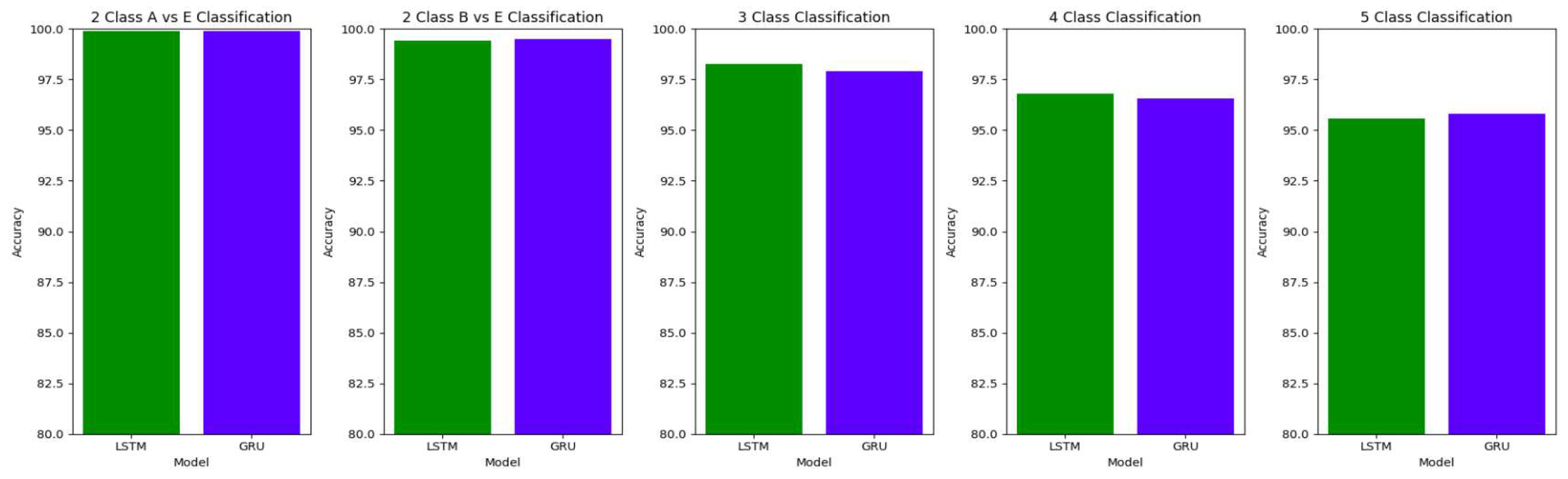
Figure 26.
Comparison of specificity between LSTM and GRU model across different classifications for filtered and segmented EEG signals of 1 s
Figure 26.
Comparison of specificity between LSTM and GRU model across different classifications for filtered and segmented EEG signals of 1 s
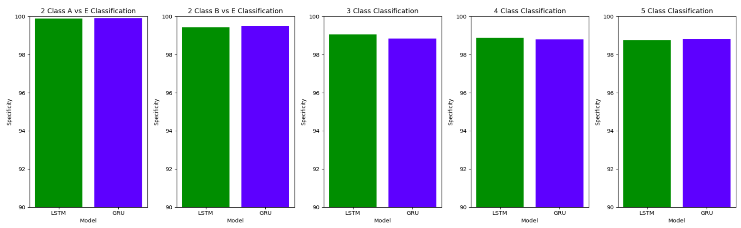
Figure 27.
Comparison of sensitivity between LSTM and GRU model across different classifications for filtered and segmented EEG signals of 1 s
Figure 27.
Comparison of sensitivity between LSTM and GRU model across different classifications for filtered and segmented EEG signals of 1 s
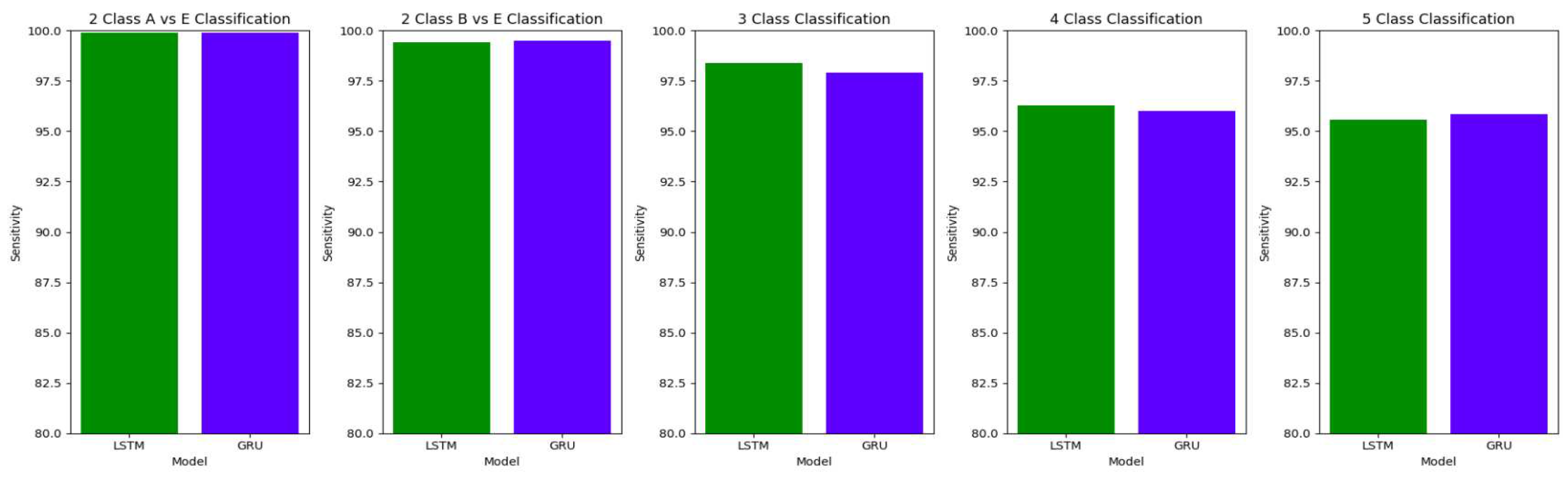
For the two-class classifications(A-E and B-E) classifications, both the LSTM and GRU models give comparable high accuracies. For the three-class classification, high accuracies are obtained for both the LSTM and the GRU models. For Study I, Study III and Study V, GRU models give slightly better accuracies of detection of epileptic seizures than LSTM models. Similarly, in the four-class classification,for Study IV, Study V and Study VI, LSTM models give better results than GRU models. In the five-class classification, LSTM and GRU models again give comparable high accuracies. The accuracies obtained are highest for the EEG signals of duration of 23.6s. For the five-class classification, the highest accuracy is achieved by Study I, obtaining an accuracy of 98%, specificity of 99.49%, sensitivity of 98.18% and F1 score of 97.94%. The accuracies obtained for the filtered as well as the unfiltered EEG signals are similar and hence, it can be said that the proposed models are robust to artifacts.
4. Discussion
In this section, we compare the performance metrics achieved by our framework with some of the work by other authors for epileptic seizure detection. The performance metrics used by the other researchers are not the same as those opted by us, hence, the comparison with other works is done on the basis of the common performance metrics.
The results obtained in our proposed work show improvement over the other research works in the detection of epilepsy. For the binary classification between healthy(set A) and seizure(set E), 100% accuracy is obtained with unfiltered EEG signals of duration 23.6s and 11.8s and filtered EEG signals of duration 23.6s. Study IV, with filtered EEG signals of duration 11.8s, gives an accuracy of 99.75%, while Study V and VI, with unfiltered and filtered EEG signals of duration 1s, respectively, give the highest accuracy of 99.16% for the LSTM model and 99.91 % for the GRU model respectively. The accuracies surpass the previous works in this field.
Similarly, for the binary classification between set B and set E, Study I, II, and III give 100% accuracy on the Bonn dataset. The Bi-LSTM model for Study IV gives 100 % accuracy in detecting seizures. Study V achieves a comparable accuracy of 99% and 99.02% for the Bi-LSTM and the Bi-GRU model, while Study VI achieves the highest accuracy of 99.5% for the B-E classification. This work shows its effectiveness in distinguishing between healthy and seizure waveforms in the binary classification. Table 14 illustrates the comparison between the proposed work and the other latest works in binary classification between normal and seizure waveforms.
Eberlein et al. [39] introduced the CNN based seizure prediction methods. They applied one-dimensional convolutions to the multi-channel iEEG signals without preprocessing or data transformation. Chandaka et al. [40] obtained an accuracy of 95.96%, an F1 Score of 93% and a sensitivity of 92% using an SVM classifier on the Bonn dataset for classification into seizure and non-seizure. Acharya et al. [41] applied a 13-layer deep CNN algorithm to an iEEG Freiburg dataset to detect normal, pre-ictal and seizure classes. They achieved an accuracy, specificity, and sensitivity of 88.67%, 90.00%, and 95.00%, respectively.
In [42], the authors have used an architecture using 1D CNN and Bidirectional LSTM to classify EEG signals into seizure and normal as well as seizure, and normal, pre-ictal and ictal. Duan et al. [43] used CNN-based spectral sub-band features related to correlation coefficients of electrodes for EEG segments of duration 1s, 2s and 3s. They achieved an accuracy of 94.8%, sensitivity of 91.7%, and specificity of 97.7%. Md.Rashed-Al-Mahefuz et al. [26] achieved the highest classification accuracy of 99.21 % using the FT-VGG16 classifier. Aarabi et al. [27] achieved an accuracy of 93%, F1 score of 95%, and a sensitivity of 91% using BNN on the Freiburg dataset. Nigam et al. [58] obtained an accuracy of 97.2% by using non-linear preprocessing filter and diagnostic neural network.
For the three-class classification between AB-CD-E(healthy-interictal-ictal), Study III with unfiltered EEG signals of duration 11.8s achieves the highest accuracy of 99.2%, specificity of 99.55%, the sensitivity of 99.14% and F1 score of 99.23%. Study I achieves an accuracy of 98.8% for the GRU model, which outperforms the LSTM model in Study I by 0.4%. Study II achieves an accuracy 98.4% for the LSTM model outperforming the GRU model. in Study IV, the maximum accuracy of 97.9 % is achieved by the LSTM model. Study V achieves the highest accuracy of 98.44% for the GRU model while Study VI obtains the highest accuracy of 98.28% for the LSTM model. Therefore, both the LSTM and GRU models perform equally well across all the studies. Therefore, the proposed framework gives an improved performance over the existing methods.
Table 15 compares the best performance metric obtained by our work with the other latest works in the field of ternary classification.
For the four-class classification, the highest accuracy of 98.4% is obtained by Study I for the GRU model. This model also gave a specificity of 99.47%, sensitivity of 98.09% and F1 score of 98.09%, outperforming the latest works in the classification of AB-C-D-E by 2.4%. All the other models in our proposed framework achieve improvements over the existing performance metrics achieved by other works. The Table 16 compares the performance of the best performance metrics obtained by the proposed work with the latest works in the field of the four-class classification.
Study I conducted with unfiltered EEG signals of duration 23.6s gives the highest classification accuracy into classes A-B-C-D-E with an accuracy of 98%, specificity of 99.49%, 98.18% and F1 score of 97.94%. An improvement by 4% over the model proposed by Turk and Ozerdem[65] is obtained by the Bi-LSTM model of Study I and an improvement by 4.4% by the Bi-GRU model of Study I. The Bi-LSTM and Bi-GRU models of Study II achieve an accuracy of 97.8% outperforming the best achieved performance by 4.2%. Study III achieves an accuracy of 96.6 % and 96.2% by the Bi-LSTM and the Bi-GRU models respectively. Study IV achieves an accuracy of 97.3% and 97% by the Bi-LSTM and Bi-GRU models again outperforming the existing methods. Table 17 illustrates the comparison between the best performance metrics obtained by the proposed work and the other research works in the 5-class classification.
5. Conclusions
This paper introduces a robust and novel framework for detecting epileptic seizures using a combination of 1D-CNN, Bidirectional LSTMs and GRUs, and Average Pooling Layer as a unit. The framework demonstrates its effectiveness in accurately distinguishing between different classes within the Bonn dataset. Extensive evaluations were conducted under both ideal and imperfect conditions, and it was found that Bidirectional LSTMs and Bidirectional GRUs yield similar results in our proposed framework. The proposed work has obtained significant advancements in the accuracy, specificity and sensitivity obtained from the existing methods for the detection of epileptic seizures, especially 3-class, 4-class and 5-class classifications. Furthermore, the proposed framework proves its efficacy in detecting epileptic seizures within EEG signals of varying durations, encompassing both longer and shorter durations. These findings highlight the suitability of the proposed framework for reliable epileptic seizure detection using EEG signals.
Author Contributions
SM and VB conceptualized the research. SM analyzed the data. VB supervised the study.SM and VB approved and contributed to writing the manuscripts. Both the authors contributed to the article and approved the submitted version.
Funding
The authors acknowledge funding support under strategic research projects from BITS BioCyTiH Foundation (a Section 8 not for profit company) hosted by BITS Pilani supported under the National Mission of Interdisciplinary Cyber Physical Systems (NM-ICPS), Department of Science & Technology (DST), Government of India.
Data Availability Statement
Data available in a publicly accessible repository. The data presented in this study are openly available in https://www.ukbonn.de/epileptologie/arbeitsgruppen/ag-lehnertz-neurophysik/ downloads/
Conflicts of Interest
The authors declare no conflict of interest.
References
- Z. Lasefr, S. S. V. N. R. Z. Lasefr, S. S. V. N. R. Ayyalasomayajula, and K. 20 October 2017. [Google Scholar]
- T. Gandhi, B. K. Panigrahi, and S. Anand, “A comparative study of wavelet families for EEG signal classification,” Neurocomputing, vol. 74, no. 17, pp. 3051–3057, 2011. [CrossRef]
- Pati, S.; Alexopoulos, A.V. Pharmacoresistant epilepsy: From pathogenesis to current and emerging therapies. Clevel. Clin. J. Med. 2010, 77, 457–467. [Google Scholar] [CrossRef]
- Sharma, R.; Pachori, R.B. Classification of epileptic seizures in EEG signals based on phase space representation of intrinsic mode functions. Expert Syst. Appl. 2015, 42, 1106–1117. [Google Scholar] [CrossRef]
- SUBASI, A. (2007) ‘EEG signal classification using wavelet feature extraction and a mixture of expert model’, Expert Systems with Applications, 32(4), pp. 1084–1093. [CrossRef]
- Loewus, D.I. (1990) ‘The Technical Writer’s Handbook. Von Matt Young. university science books, Mill Valley, CA, 1989. XI, 232 S., geb., $ 25.00. – ISBN 0-935702-60-1’, Angewandte Chemie, 102(1), pp. 115–116. [CrossRef]
- Akter, M.; Islam, R.; Tanaka, T.; Iimura, Y.; Mitsuhashi, T.; Sugano, H.; Wang, D.; Molla, K.I. Statistical Features in High-Frequency Bands of Interictal iEEG Work Efficiently in Identifying the Seizure Onset Zone in Patients with Focal Epilepsy. Entropy 2020, 22, 1415. [Google Scholar] [CrossRef] [PubMed]
- Kotiuchyi, I.; Pernice, R.; Popov, A.; Faes, L.; Kharytonov, V. A Framework to Assess the Information Dynamics of Source EEG Activity and Its Application to Epileptic Brain Networks. Brain Sci. 2020, 10, 657. [Google Scholar] [CrossRef]
- Yann. LeCun and Yoshua. Bengio. Convolutional networks for images, speech, and timeseries. In M. A. Arbib, editor, The Handbook of Brain Theory and Neural Networks. MIT Press, 1995.
- Y. Bengio, P. Y. Bengio, P. Simard, and P. Frasconi, “Learning Long-Term Dependencies with Gradient Descent is Difficult,” IEEE Trans. Neural Networks, vol. 5, no. 2, pp. 157–166, 1994.
- R. Pascanu, T. R. Pascanu, T. Mikolov, and Y. Bengio, “On the difficulty of training recurrent neural networks,” in International Conference on Machine Learning, 2013, no. 2, pp. 1310–1318.
- Najafi, T.; Jafaar, R.; Remli, R.; Chellappan, K. The Role of Brain Signal Processing and Neuronal Modeling in Epilepsy. In Proceedings of the International Epilepsy Day, Malaysia, 4 February 2021. [Google Scholar]
- Duque-Muñoz, L.; Espinosa-Oviedo, J.J.; Castellanos-Dominguez, C.G. Identification and monitoring of brain activity based on stochastic relevance analysis of short-time EEG rhythms. Biomed. Eng. Online 2014, 13, 1–20. [Google Scholar] [CrossRef] [PubMed]
- Oweis, R.J.; Abdulhay, E.W. Seizure classification in EEG signals utilizing Hilbert-Huang transform. Biomed. Eng. Online 2011, 10, 38. [Google Scholar] [CrossRef]
- Chen, D.; Wan, S.; Xiang, J.; Bao, F.S. A high-performance seizure detection algorithm based on Discrete Wavelet Transform (DWT) and EEG. PLoS ONE 2017, 12, 1–21. [Google Scholar] [CrossRef]
- Riaz, F.; Hassan, A.; Rehman, S.; Niazi, I.K.; Dremstrup, K. EMD-based temporal and spectral features for the classification of EEG signals using supervised learning. IEEE Trans. Neural Syst. Rehabil. Eng. 2016, 24, 28–35. [Google Scholar] [CrossRef] [PubMed]
- Ihsan Ullah, Muhammad Hussain, Emad-ul-Haq Qazi, Hatim Aboalsamh, An automated system for epilepsy detection using EEG brain signals based on deep learning approach, Expert Systems with Applications, Volume 107, 2018,Pages 61-71, ISSN 0957-417. Available online: https://www.sciencedirect.com/science/article/pii/S0957417418302513. [CrossRef]
- Roy, S. , Kiral-Kornek, I. & Harrer, S. ChronoNet: A Deep Recurrent Neural Network for Abnormal EEG Identification. 2018. [Google Scholar] [CrossRef]
- Ramy Hussein, Hamid Palangi, Rabab K. Ward, Z. Jane Wang, Optimized deep neural network architecture for robust detection of epileptic seizures using EEG signals, Clinical Neurophysiology, Volume 130, Issue 1, 2019, Pages 25-37, ISSN 1388-2457. Available online: https://www.sciencedirect.com/science/article/pii/S1388245718313464. [CrossRef]
- Thara D.K., PremaSudha B.G., Fan Xiong, Epileptic seizure detection and prediction using stacked bidirectional long short term memory, Pattern Recognition Letters, Volume 128, 2019, Pages 529-535, ISSN 0167-8655. Available online: https://www.sciencedirect.com/science/article/pii/S0167865519303125.
- G. R. Minasyan, J. B. Chatten, and M. J. Chatten. 2010. Patient-specific early seizure detection from scalp EEG. Journal of Clinical Neurophysiology: Official Publication of the American Electroencephalographic Society 27, 3.
- Quang, M. Tieng, Irina Kharatishvili, Min Chen, and David C Reutens. 2016. Mouse EEG spike detection based on the adapted continuous wavelet transform. Journal of Neural Engineering 13, 2 (2016), 026018. [CrossRef]
- Siddharth Pramod, Adam Page, Tinoosh Mohsenin, and Tim Oates. 2014. Detecting epileptic seizures from EEG data using neural networks. arXiv 2014, arXiv:1412.6502.
- Turner, J.J. et al. (2014) Deep Belief Networks used on High Resolution Multichannel Electroencephalography Data for Seizure Detection, arXiv (Cornell University). Cornell University. Available online: https://arxiv.org/abs/1708.08430.
- Alexander Rosenberg Johansen, Jing Jin, Tomasz Maszczyk, and Justin Dauwels. 2016. Epileptiform spike detection via convolutional neural networks. In 2016 IEEE International Conference on Acoustics, Speech and Signal Processing (ICASSP).
- Rashed-Al-Mahfuz, M.; Moni, M.A.; Uddin, S.; Alyami, S.A.; Summers, M.A.; Eapen, V. A deep convolutional neural network method to detect seizures and characteristic frequencies using epileptic electroencephalogram (EEG) data. IEEE J. Transl. Eng. Health Med. 2021, 9, 1–12. [Google Scholar] [CrossRef]
- Aarabi, A.; Fazel-Rezai, R.; Aghakhani, Y. A fuzzy rule-based system for epileptic seizure detection in intracranial EEG. Clin. Neurophysiol. 2009, 120, 1648–1657. [Google Scholar] [CrossRef]
- Andreas Antoniades, Loukianos Spyrou, Clive Cheong Took, and Saeid Sanei. 2016. Deep learning for epileptic intracranial EEG data. In 2016 IEEE 26th International Workshop on Machine Learning for Signal Processing (MLSP). IEEE, 1–6.
- Sharan, R. V. , & Berkovsky, S. (2020). Epileptic Seizure Detection Using Multi-Channel EEG Wavelet Power Spectra and 1-D Convolutional Neural Networks. Annual International Conference of the IEEE Engineering in Medicine and Biology Society. IEEE Engineering in Medicine and Biology Society. Annual International Conference, 2020, 545–548. [CrossRef]
- R. G. Andrzejak, K. Lehnertz, F. Mormann, C. Rieke, P. David, and C. E. Elger, “Indications of nonlinear deterministic and finite-dimensional structures in time series of brain electrical activity: Dependence on recording region and brain state,” Physical Review E, vol. 64, no. 6, p. 061907, 2001. [CrossRef]
- Kuanar, S.; Athitsos, V.; Pradhan, N.; Mishra, A.; Rao, K. Cognitive Analysis of Working Memory Load from Eeg, by a Deep Recurrent Neural Network. In Proceedings of the 2018 IEEE International Conference on Acoustics, Speech and Signal Processing (ICASSP), Calgary, AB, Canada, 15–20 April 2018; pp. 2576–2580. [Google Scholar]
- S. Albawi, T. A. S. Albawi, T. A. Mohammed and S. Al-Zawi, "Understanding of a convolutional neural network," 2017 International Conference on Engineering and Technology (ICET), Antalya, Turkey, 2017, pp. -6. [CrossRef]
- Shoeibi A, Khodatars M, Ghassemi N, Jafari M, Moridian P, Alizadehsani R, Panahiazar M, Khozeimeh F, Zare A, Hosseini-Nejad H, Khosravi A, Atiya AF, Aminshahidi D, Hussain S, Rouhani M, Nahavandi S, Acharya UR. Epileptic Seizures Detection Using Deep Learning Techniques: A Review. International Journal of Environmental Research and Public Health. 2021; 18(11):5780. [CrossRef]
- S. Hochreiter, S. S. Hochreiter, S. Hochreiter, J. Schmidhuber, and J. Schmidhuber, “Long short-term memory.,” Neural Comput., vol. 9, no. 8, pp. 1735–80, 1997.
- Nagabushanam, P.; George, S.T.; Radha, S. EEG signal classification using LSTM and improved neural network algorithms. Soft Comput. 2020, 24, 9981–10003. [Google Scholar] [CrossRef]
- J. Chung, C. J. Chung, C. Gulcehre, K. Cho, and Y. Bengio, “Empirical Evaluation of Gated Recurrent Neural Networks on Sequence Modeling,” arXiv Prepr. arXiv1412.3555, pp. 1–9, 2014.
- Srivastava, Nitish, et al. "Dropout: a simple way to prevent neural networks from overfitting." The journal of machine learning research 15.1 (2014): 1929-1958.
- Islam, M.K.; Rastegarnia, A.; Yang, Z. Methods for artifact detection and removal from scalp EEG: A review. Clin. Neurophysiol. 2016, 46, 287–305. [Google Scholar] [CrossRef]
- Schirrmeister, R. T. , Springenberg, J. T., Fiederer, L. D. J., Glasstetter, M., Eggensperger, K., Tangermann, M., Hutter, F., Burgard, W.,& Ball, T. (2017). Deep learning with convolutional neural networks for EEG decoding and visualization. Human brain mapping, 38(11), 5391–5420. [CrossRef]
- Chandaka, S.; Chatterjee, A.; Munshi, S. Cross-correlation aided support vector machine classifier for classification of EEG signals. Expert Syst. Appl. 2009, 36, 1329–1336. [Google Scholar] [CrossRef]
- Acharya, U. R. , Hagiwara, Y., & Adeli, H. (2018). Automated seizure prediction. Epilepsy & behavior : E&B, 88, 251–261. [CrossRef]
- Abdelhameed, A. , Daoud, H. & Bayoumi, M. Deep Convolutional Bidirectional LSTM Recurrent Neural Network for Epileptic Seizure Detection. 2018 16th IEEE International New Circuits And Systems Conference (NEWCAS), 2018. [Google Scholar]
- Duan L, Hou J, Qiao Y, Miao J (2019) Epileptic seizure prediction based on convolutional recurrent neural network with multi-timescale. Intelligence science and big data engineering. Big data and machine learning.
- K. Abualsaud, M. K. Abualsaud, M. Mahmuddin, M. Saleh, and A. Mohamed, “Ensemble classifier for epileptic seizure detection for imperfect EEG data,” The Scientific World Journal, vol. 2015, 2015. [CrossRef]
- Subasi, A.; Erçelebi, E. Classification of EEG signals using neural network and logistic regression. Comput. Methods Programs Biomed. 2005, 78, 87–99. [Google Scholar] [CrossRef] [PubMed]
- Shoeibi, A.; Ghassemi, N.; Khodatars, M.; Moridian, P.; Alizadehsani, R.; Zare, A.; Gorriz, J.M. Detection of Epileptic Seizures on EEG Signals Using ANFIS Classifier, Autoencoders and Fuzzy Entropies. arXiv arXiv:2109.04364, 2021. [CrossRef]
- Ghosh-Dastidar, S.; Adeli, H. Improved spiking neural networks for EEG classification and epilepsy and seizure detection. Integr. Comput. Aided Eng. 2017, 14, 187–212. [Google Scholar] [CrossRef]
- Ghosh-Dastidar, S.; Adeli, H. A new supervised learning algorithm for multiple spiking neural networks with application in epilepsy and seizure detection. Neural Netw. 2009, 22, 1419–1431. [Google Scholar] [CrossRef]
- Chua, K.C.; Chandran, V.; Acharya, U.R.; Lim, C.M. Application of higher order spectra to identify epileptic EEG. J. Med. Syst. 2010, 35, 1563–1571. [Google Scholar] [CrossRef] [PubMed]
- Acharya, U.R.; Sree, S.V.; Ang, P.C.A.; Suri, J.S. Use of principal component analysis for automatic detection of epileptic EEG activities. Expert Syst. Appl. 2012, 39, 9072–9078. [Google Scholar] [CrossRef]
- Vipani, R.; Hore, S.; Basu, S.; Basak, S.; Dutta, S. Identification of Epileptic Seizures Using Hilbert Transform and Learning Vector Quantization Based Classifier. In Proceedings of the IEEE Calcutta Conference (CALCON), Kalkata, India, 2–3 December 2017; pp. 90–94. [Google Scholar]
- Akyol, K. Stacking ensemble based deep neural networks modeling for effective epileptic seizure detection. Expert Syst. Appl. 2020, 148, 113239. [Google Scholar] [CrossRef]
- Gupta, V.; Pachori, R.B. Epileptic seizure identification using entropy of FBSE based EEG rhythms. Biomed. Signal Process. Control. 2019, 53, 101569. [Google Scholar] [CrossRef]
- Abiyev, R.; Arslan, M.; Bush Idoko, J.; Sekeroglu, B.; Ilhan, A. Identification of Epileptic EEG Signals Using Convolutional Neural Networks. Appl. Sci. 2020, 10, 4089. [Google Scholar] [CrossRef]
- Kaya, Y.; Uyar, M.; Tekin, R.; Yıldırım, S. 1D-local binary pattern based feature extraction for classification of epileptic EEG signals. Appl. Math. Comput. 2014, 243, 209–219. [Google Scholar] [CrossRef]
- Tzallas, A.; Tsipouras, M.; Fotiadis, D. Automatic seizure detection based on time-frequency analysis and artificial neural networks. Comput. Intell. Neurosci. 2007, 2007, 80510. [Google Scholar] [CrossRef] [PubMed]
- Bhattacharyya, A.; Pachori, R.B.; Upadhyay, A.; Acharya, U.R. Tunable-Q Wavelet Transform Based Multiscale Entropy Measure for Automated Classification of Epileptic EEG Signals. Appl. Sci. 2017, 7, 385. [Google Scholar] [CrossRef]
- Nigam, V.P. and Graupe, D., 2004. A neural-network-based detection of epilepsy. Neurological research, 26(1), pp.55-60. [CrossRef]
- Samiee, K.; Kovács, P.; Gabbouj, M. Epileptic seizure classification of EEG time-series using rational discrete short-time Fourier transform. IEEE Trans. Biomed. Eng. 2015, 62, 541–552. [Google Scholar] [CrossRef] [PubMed]
- Orhan, U.; Hekim, M.; Ozer, M. EEG signals classification using the K-means clustering and a multilayer perceptron neural network model. Expert Syst. Appl. 2011, 38, 13475–13481. [Google Scholar] [CrossRef]
- Peker, M.; Sen, B.; Delen, D. A novel method for automated diagnosis of epilepsy using complex-valued classifiers. IEEE J. Biomed. Health Inform. 2016, 20, 108–118. [Google Scholar] [CrossRef]
- S. Fawad Hussain and S. Mian Qaisar, “Epileptic seizure classification using level-crossing EEG sampling and ensemble of sub-problems classifier,” Expert Systems with Applications, vol. 191, Article ID 116356, 2022. [CrossRef]
- Hassan, F. , Hussain, S.F. and Qaisar, S.M. (2022) ‘Epileptic seizure detection using a hybrid 1D CNN-machine learning approach from EEG Data’, Journal of Healthcare Engineering, 2022, pp. 1–16. [CrossRef]
- A. Zahra, N. A. Zahra, N. Kanwal, N. ur Rehman, S. Ehsan, and K. D. McDonald-Maier, “Seizure detection from EEG signals using multivariate empirical mode decomposition,” Computers in Biology and Medicine, vol. 88, pp. 132–141, 2017. [CrossRef]
- O. Turk and M. S. Ozerdem, “Epilepsy detection by using scalogram based convolutional neural network from EEG signals,” Brain Sciences, vol. 9, no. 5, Article ID 115, 2019. [CrossRef]
Figure 1.
EEG Signals : (a) EEG Signals from set A or Z : Healthy patients with eyes opened (b) EEG signals from set B or O: Healthy patients with eyes closed (c) EEG signals from set C or N : inter-ictal from seizure-free intervals; recorded from a region opposite to the epileptogenic zone (d) EEG signals from set D or F: inter-ictal from seizure-free intervals; recording EEG signals from the epileptogenic zone (e) EEG signals from set E or S: seizure waveforms
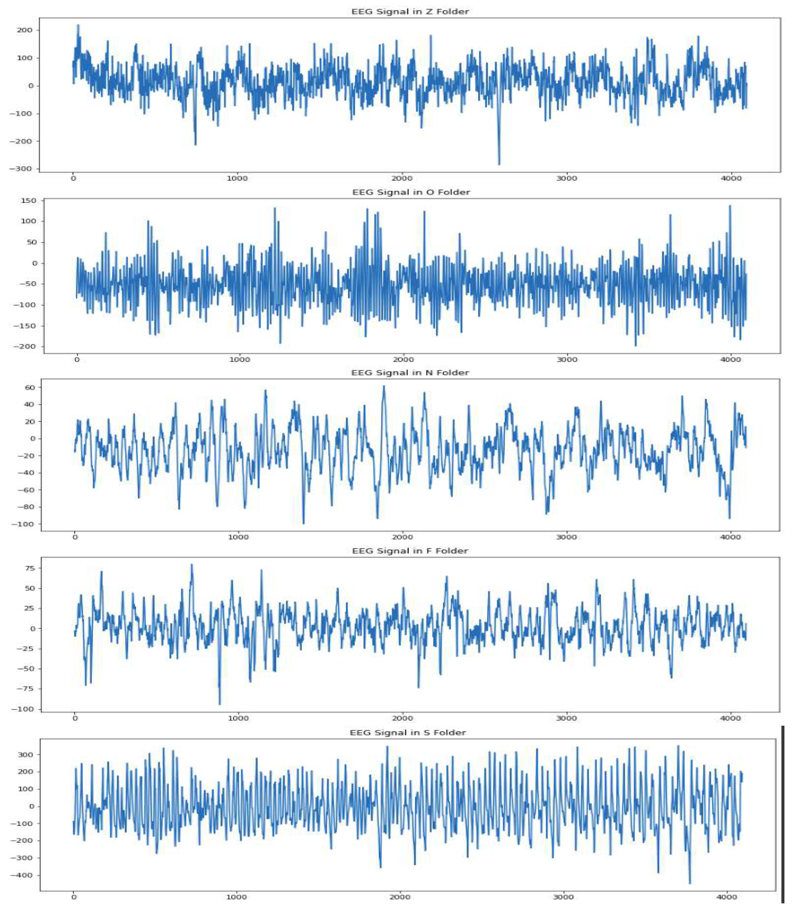
Figure 2.
Proposed framework for the detection of epileptic seizures from EEG signals
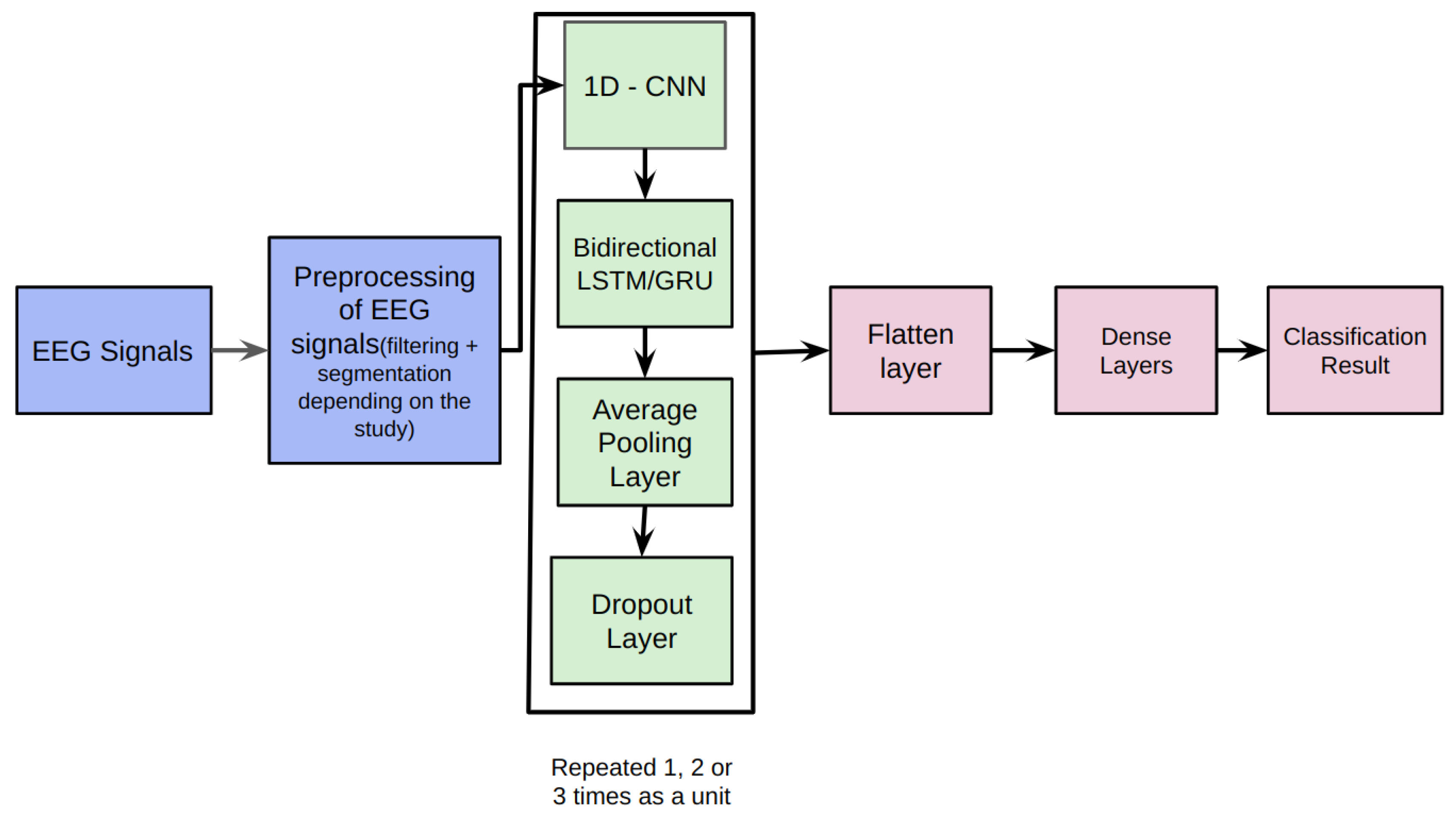
Figure 3.
Architecture of LSTM cell
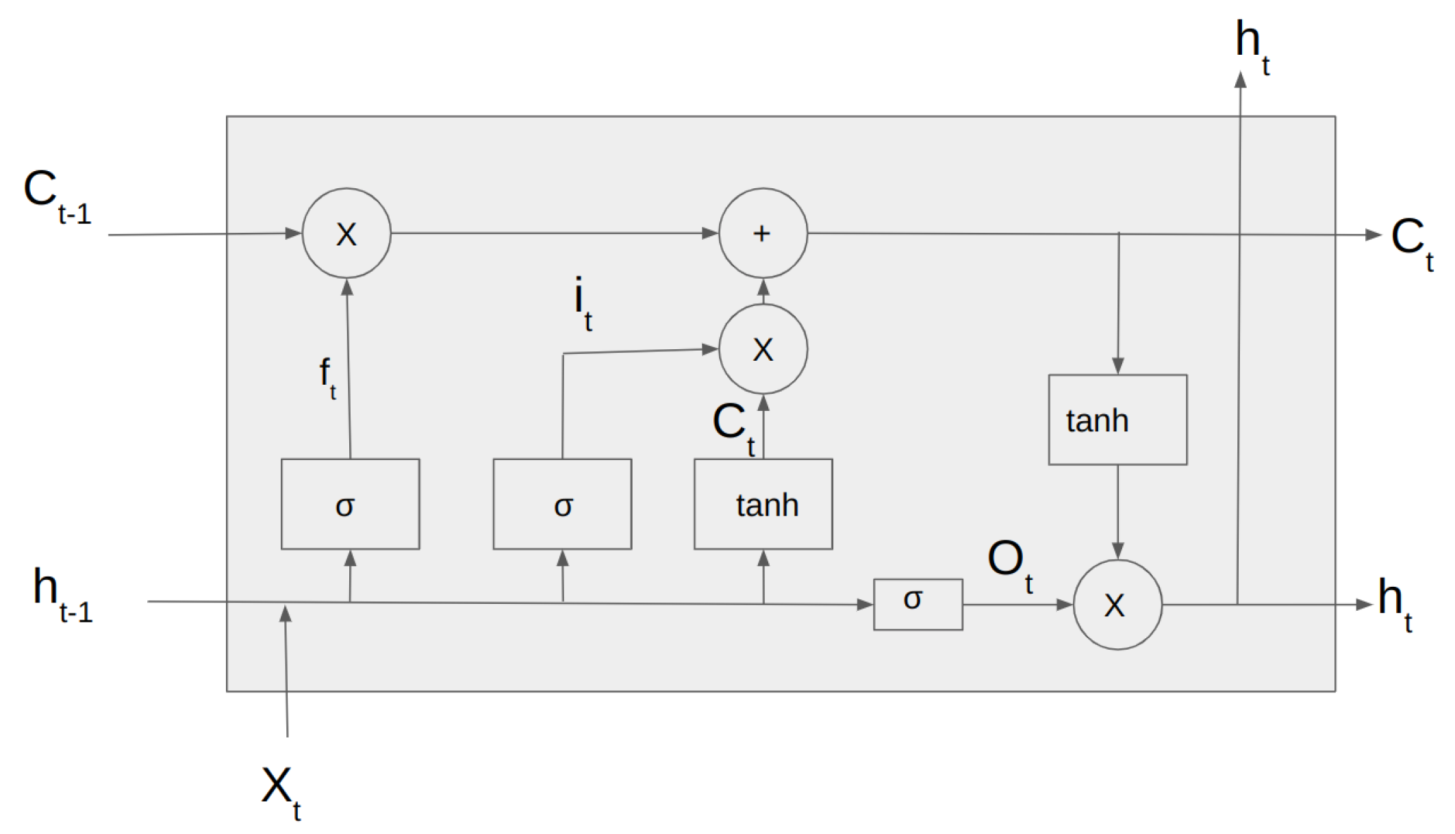
Figure 4.
Architecture of GRU cell
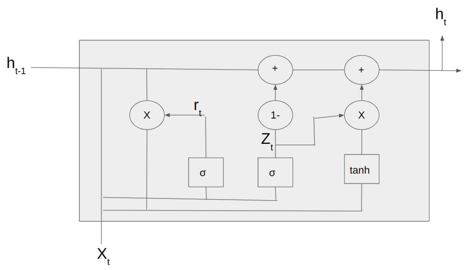
Figure 5.
Pipeline of Study II: Using filtered EEG signals of duration 23.6s
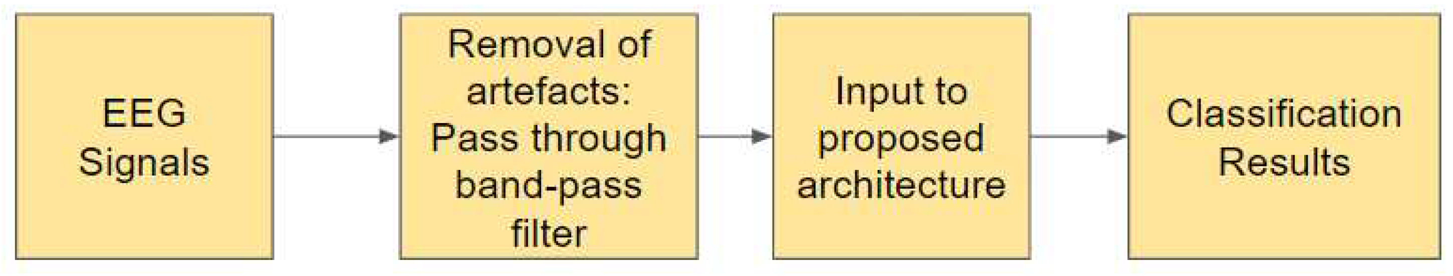
Figure 6.
Pipeline of Study III: Using raw EEG signals of duration 11.8s
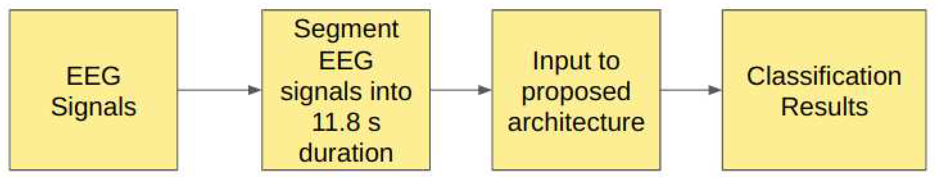
Figure 7.
Pipeline of Study IV: Using filtered EEG signals of duration 11.8s
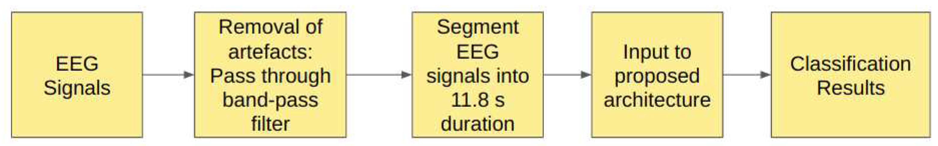
Figure 8.
Pipeline of Study V: Using raw EEG signals of duration 1s
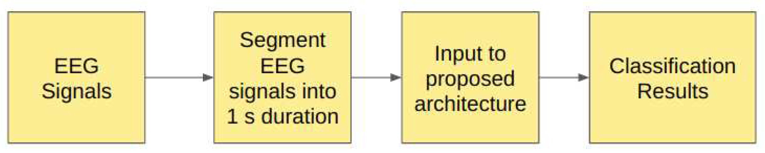
Figure 9.
Pipeline of Study VI: Using filtered EEG signals of duration 1s
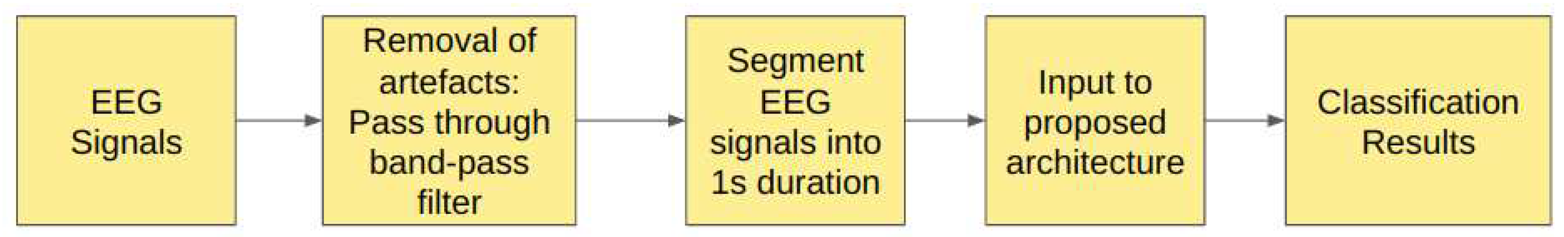
Figure 10.
Comparison of accuracy between LSTM and GRU model across different classifications for unfiltered EEG signals of duration 23.6s
Figure 10.
Comparison of accuracy between LSTM and GRU model across different classifications for unfiltered EEG signals of duration 23.6s
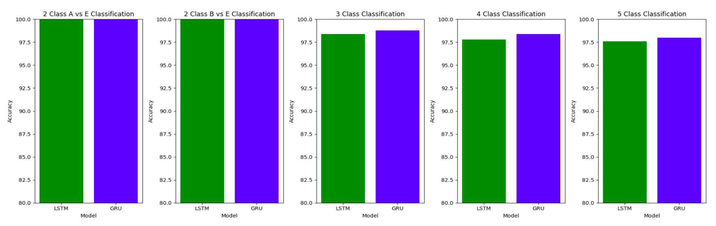
Figure 11.
Comparison of specificity between LSTM and GRU model across different classifications for unfiltered EEG signals of duration 23.6s
Figure 11.
Comparison of specificity between LSTM and GRU model across different classifications for unfiltered EEG signals of duration 23.6s
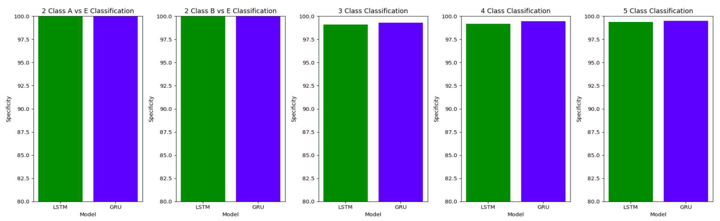
Figure 12.
Comparison of sensitivity between LSTM and GRU model across different classifications for unfiltered EEG signals of duration 23.6s
Figure 12.
Comparison of sensitivity between LSTM and GRU model across different classifications for unfiltered EEG signals of duration 23.6s
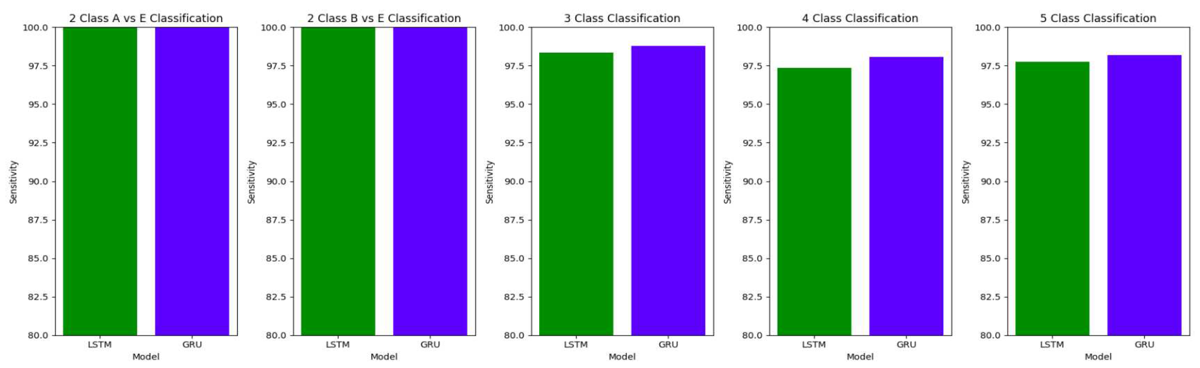
Figure 13.
Comparison of accuracy between LSTM and GRU model across different classifications for filtered EEG signals of duration 23.6s
Figure 13.
Comparison of accuracy between LSTM and GRU model across different classifications for filtered EEG signals of duration 23.6s
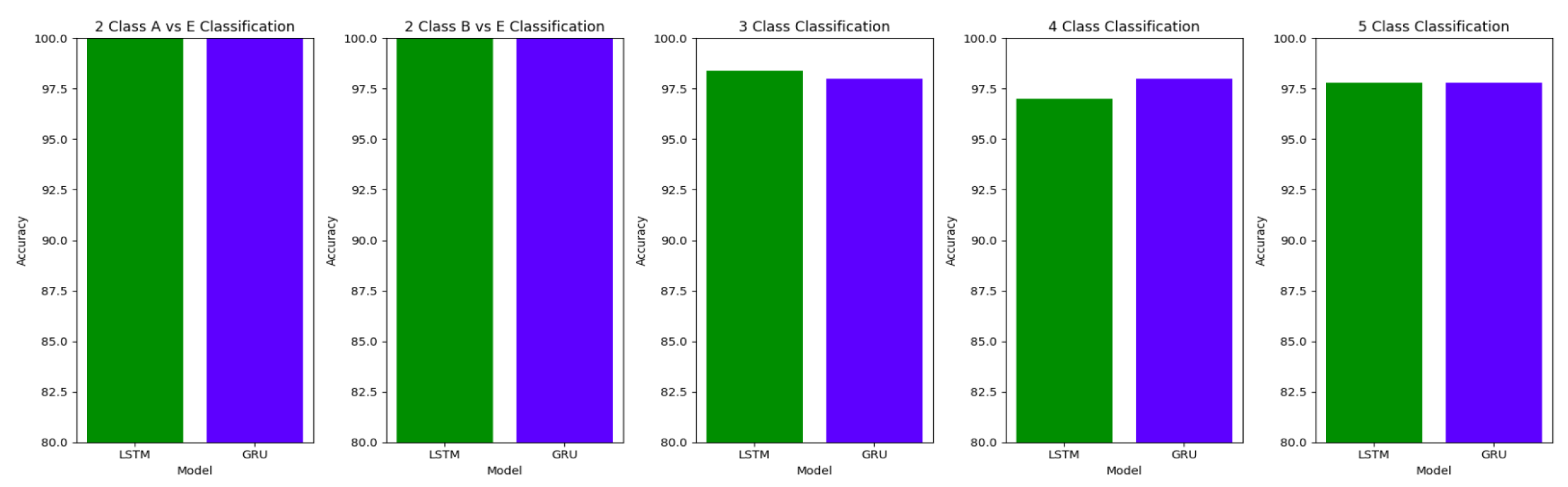
Figure 14.
Comparison of specificity between LSTM and GRU model across different classifications for filtered EEG signals of duration 23.6s
Figure 14.
Comparison of specificity between LSTM and GRU model across different classifications for filtered EEG signals of duration 23.6s
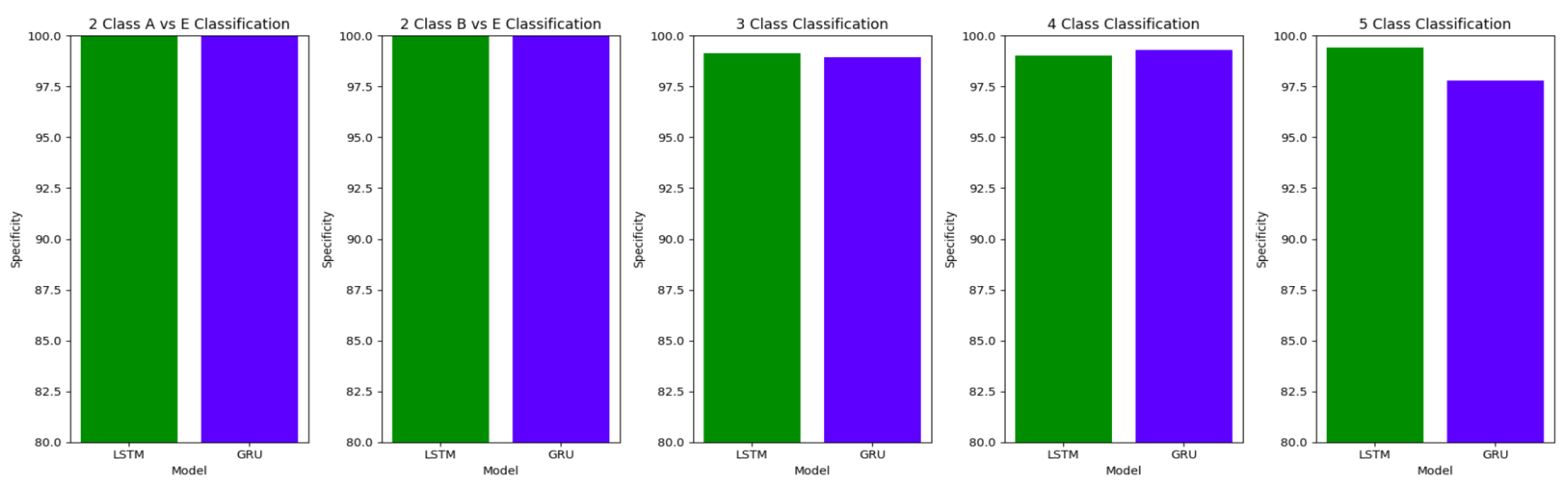
Figure 15.
Comparison of sensitivity between LSTM and GRU model across different classifications for filtered EEG signals of duration 23.6s
Figure 15.
Comparison of sensitivity between LSTM and GRU model across different classifications for filtered EEG signals of duration 23.6s
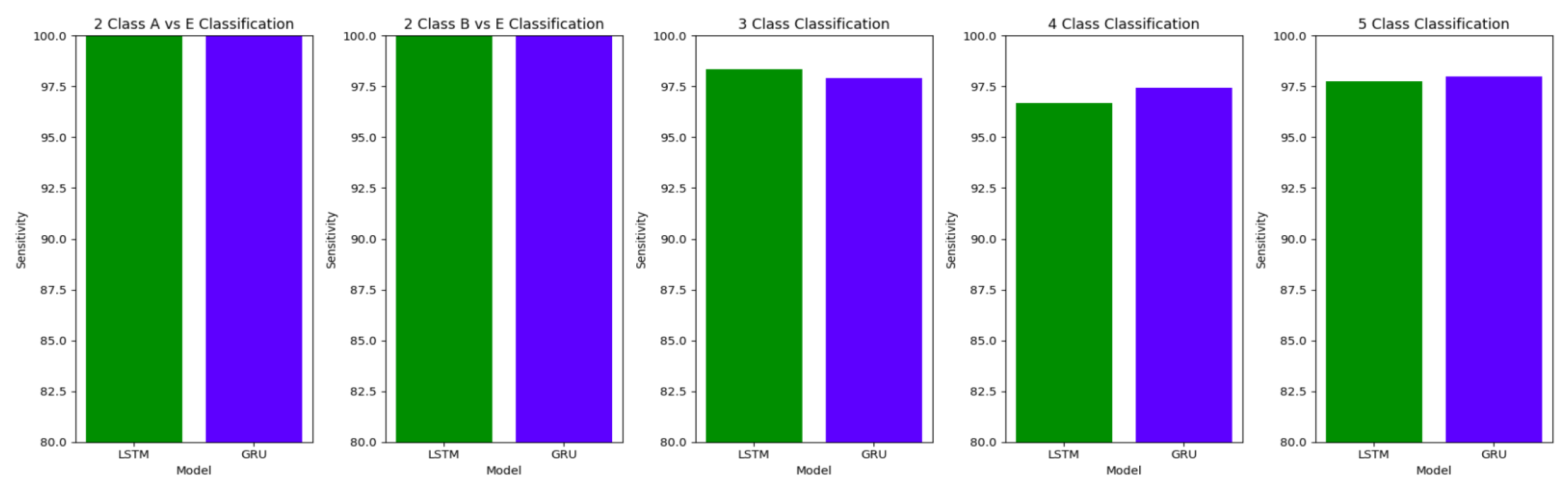
Figure 16.
Comparison of accuracy between LSTM and GRU model across different classifications for unfiltered and segmented EEG signals of 11.8 s
Figure 16.
Comparison of accuracy between LSTM and GRU model across different classifications for unfiltered and segmented EEG signals of 11.8 s
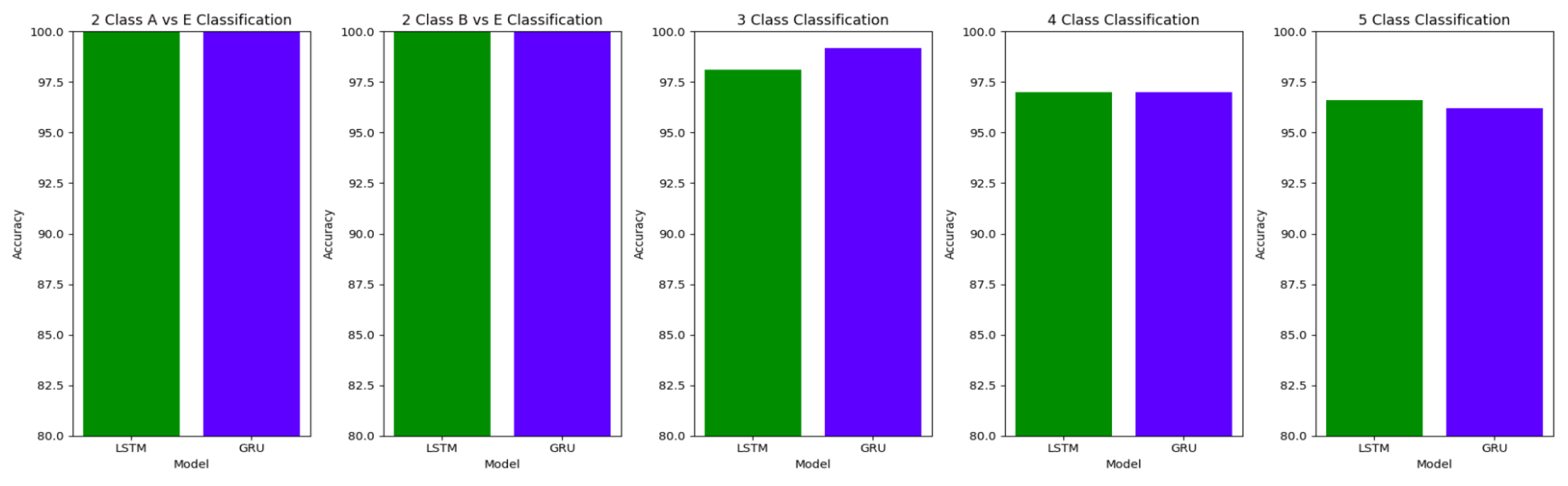
Figure 17.
Comparison of specificity between LSTM and GRU model across different classifications for unfiltered and segmented EEG signals of 11.8 s
Figure 17.
Comparison of specificity between LSTM and GRU model across different classifications for unfiltered and segmented EEG signals of 11.8 s
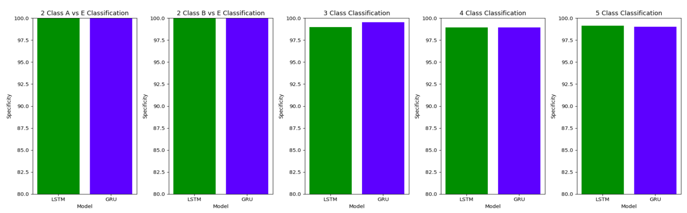
Figure 18.
Comparison of sensitivity between LSTM and GRU model across different classifications for unfiltered and segmented EEG signals of 11.8 s
Figure 18.
Comparison of sensitivity between LSTM and GRU model across different classifications for unfiltered and segmented EEG signals of 11.8 s
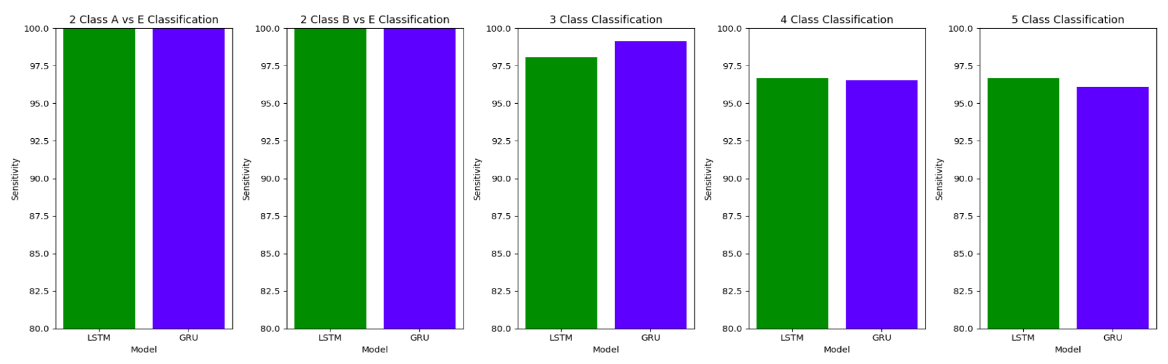
Figure 19.
Comparison of accuracy between LSTM and GRU model across different classifications for filtered and segmented EEG signals of 11.8 s
Figure 19.
Comparison of accuracy between LSTM and GRU model across different classifications for filtered and segmented EEG signals of 11.8 s
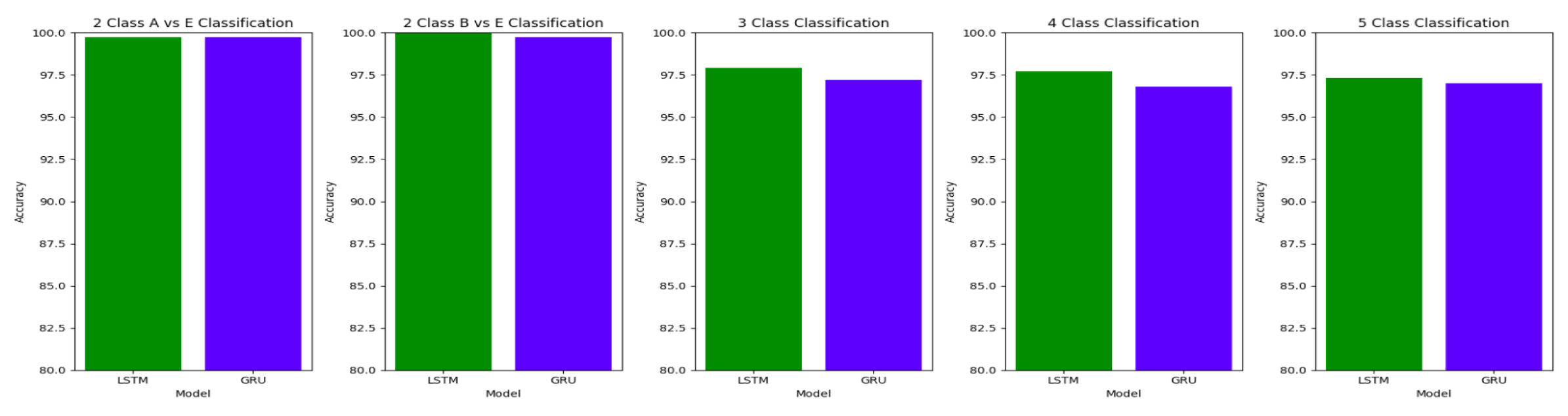
Figure 20.
Comparison of specificity between LSTM and GRU model across different classifications for filtered and segmented EEG signals of 11.8 s
Figure 20.
Comparison of specificity between LSTM and GRU model across different classifications for filtered and segmented EEG signals of 11.8 s
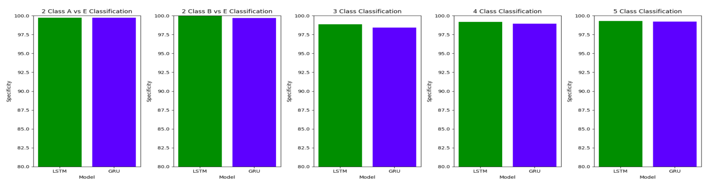
Figure 21.
Comparison of sensitivity between LSTM and GRU model across different classifications for filtered and segmented EEG signals of 11.8 s
Figure 21.
Comparison of sensitivity between LSTM and GRU model across different classifications for filtered and segmented EEG signals of 11.8 s
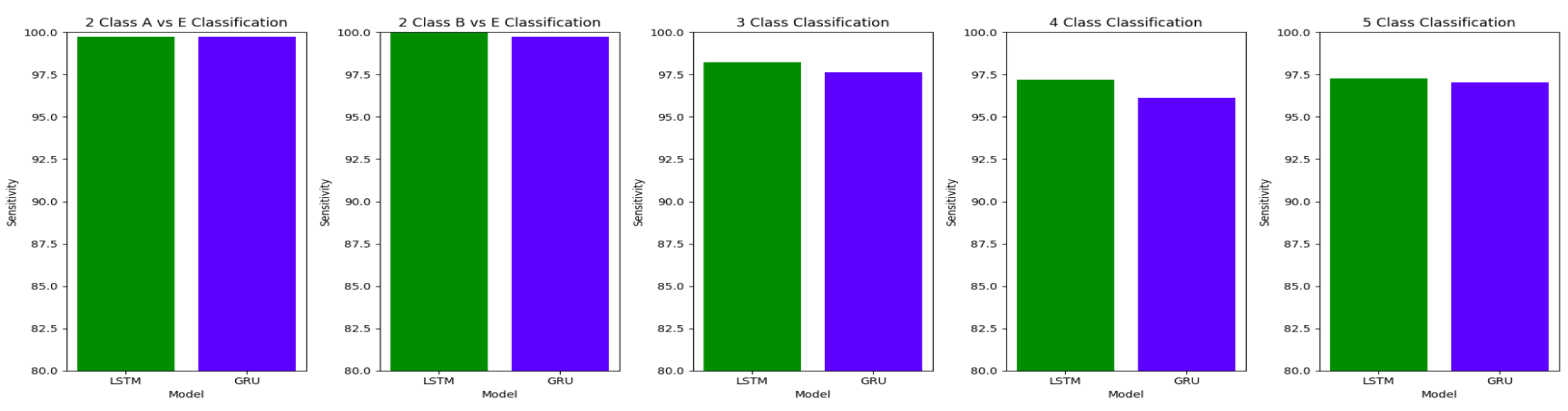
Figure 22.
Comparison of accuracy between LSTM and GRU model across different classifications for unfiltered and segmented EEG signals of 1 s
Figure 22.
Comparison of accuracy between LSTM and GRU model across different classifications for unfiltered and segmented EEG signals of 1 s
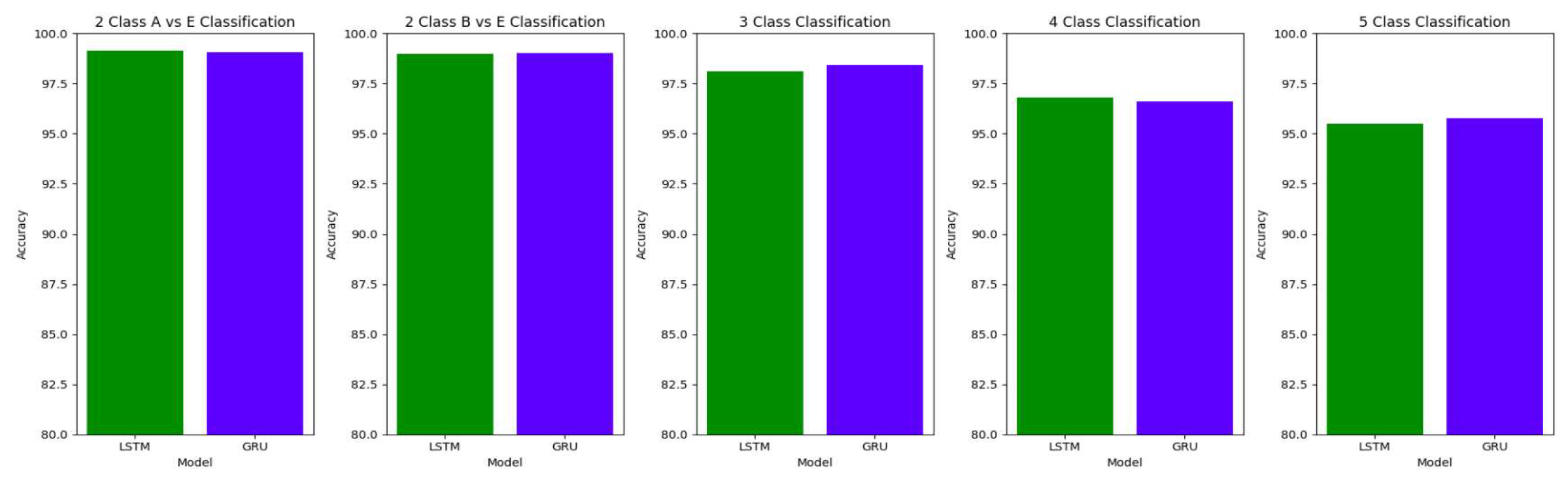
Figure 23.
Comparison of specificity between LSTM and GRU model across different classifications for unfiltered and segmented EEG signals of 1 s
Figure 23.
Comparison of specificity between LSTM and GRU model across different classifications for unfiltered and segmented EEG signals of 1 s
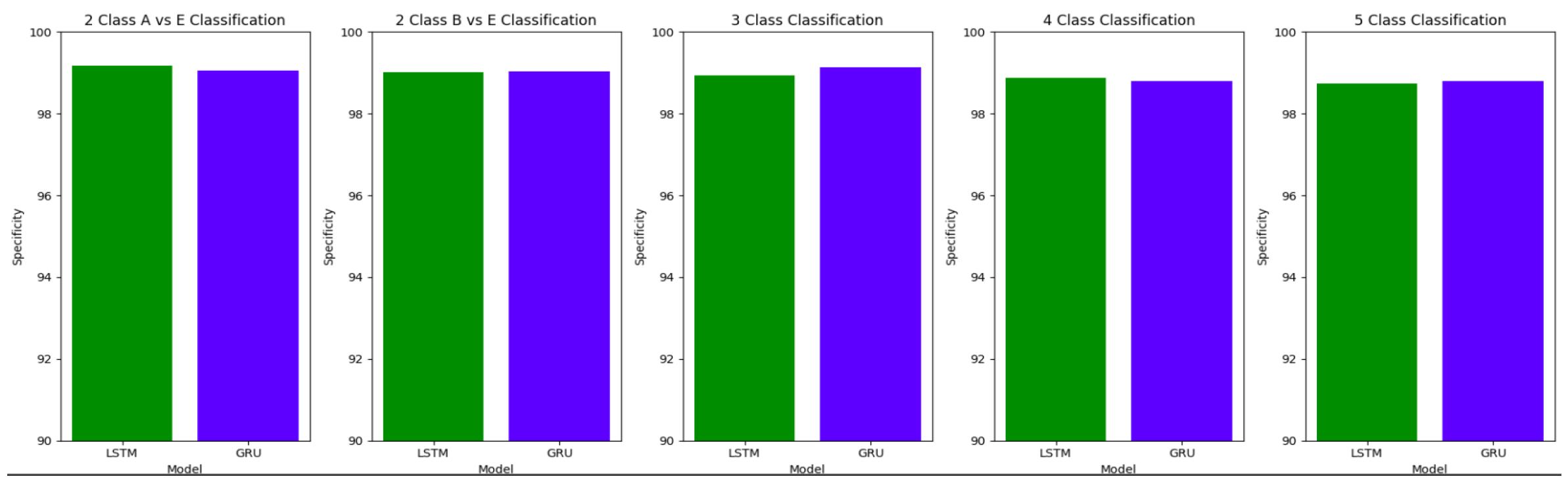
Figure 24.
Comparison of sensitivity between LSTM and GRU model across different classifications for unfiltered and segmented EEG signals of 1 s
Figure 24.
Comparison of sensitivity between LSTM and GRU model across different classifications for unfiltered and segmented EEG signals of 1 s
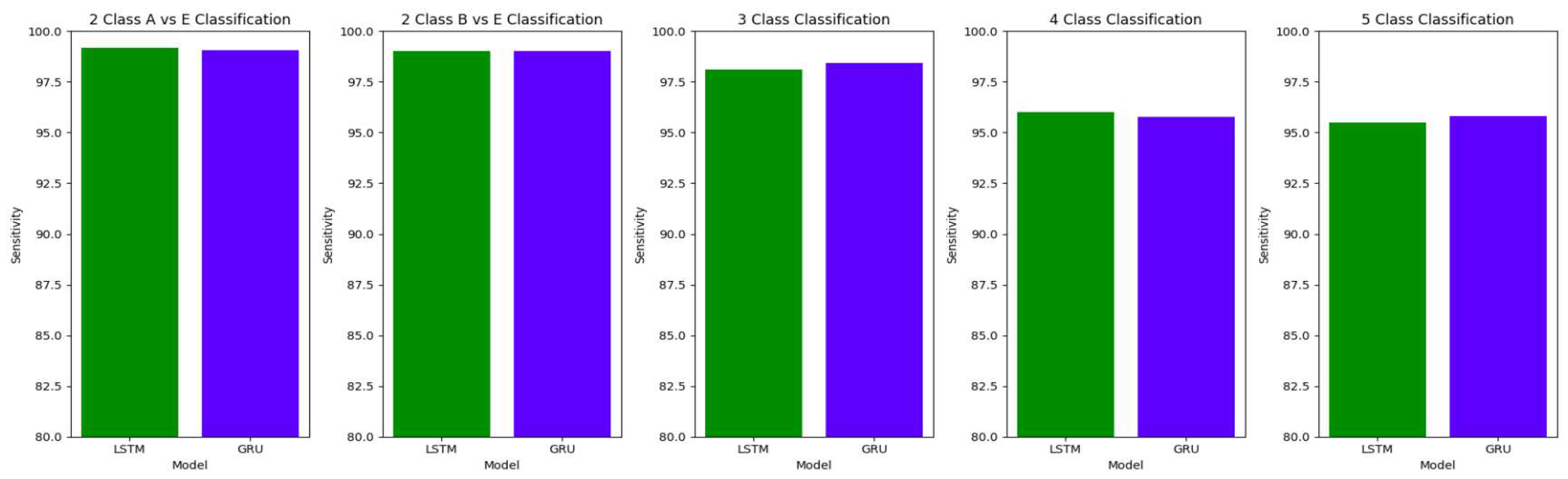

Table 1.
Classification Type and Set Combination used in the study
| Classification Type | Data Combination |
|---|---|
| Two Class Classification | A vs. E |
| Two Class Classification | B vs. E |
| Three Class Classification | AB vs. CD vs. E |
| Four Class Classification | AB vs. C vs. D vs. E |
| Five Class Classification | A vs B vs C vs D vs E |
Table 2.
Details of proposed model
| Type of Classification |
Conv1D(1) | LSTM(1) / GRU(1) |
Conv1D(2) | LSTM(2) / GRU(2) |
Conv1D(3) | LSTM(3) / / GRU(3) |
Dropout after each unit |
Learning Rate |
No.of epochs |
Batch Size |
|---|---|---|---|---|---|---|---|---|---|---|
| A-E | 128 | 128 | - | - | - | - | 0.1 | 0.001 | 50 | 64 |
| B-E | 32 | 32 | 16 | 16 | - | - | 0.1 | 0.001 | 100 | 64 |
| AB-CD-E | 64 | 8 | 128 | 4 | - | - | 0.1 | 0.001 | 150 | 64 |
| AB-C-D-E | 128 | 32 | 64 | 16 | 32 | 8 | 0.1 | 0.001 | 150 | 64 |
| A-B-C-D-E | 128 | 32 | 64 | 16 | 32 | 8 | 0.1 | 0.001 | 150 | 64 |
Table 3.
Details of proposed model
| Type of Classification |
Conv1D(1) | LSTM(1) / GRU(1) |
Conv1D(2) | LSTM(2) / GRU(2) |
Conv1D(3) | LSTM(3) /GRU(3) |
Dropout | Learning Rate | No.of epochs | Batch Size |
|---|---|---|---|---|---|---|---|---|---|---|
| A-E | 4 | 8 | 4 | 8 | - | - | 0.1 | 0.001 | 150 | 64 |
| B-E | 32 | 32 | 16 | 16 | - | - | 0.1 | 0.001 | 100 | 64 |
| AB-CD-E | 256 | 128 | 64 | 64 | 32 | 32 | 0.1 | 0.0005 | 150 | 64 |
| AB-C-D-E | 64 | 64 | 32 | 32 | 16 | 16 | 0.1 | 0.0005 | 150 | 64 |
| A-B-C-D-E | 128 | 64 | 64 | 32 | 32 | 16 | 0.1 | 0.0001 | 150 | 64 |
Table 4.
Details of proposed models for Study III
| Type of Classification |
Conv1D(1) | LSTM(1) /GRU(1) |
Conv1D(2) | LSTM(2)/ GRU(2) |
Conv1D(3) | LSTM(3)/ GRU(3) |
Conv1D(4) | LSTM (4)/ GRU(4) |
Dropout after each unit |
Learning Rate |
|---|---|---|---|---|---|---|---|---|---|---|
| A-E | 256 | 64 | 64 | 32 | 32 | 16 | 0.1 | - | - | 0.001 |
| B-E | 256 | 64 | 64 | 32 | 32 | 16 | 0.1 | - | - | 0.001 |
| AB-CD-E | 32 | 16 | 16 | 8 | 8 | 4 | 0.1 | - | - | 0.0005 |
| AB-C-D-E | 256 | 32 | 128 | 32 | 64 | 16 | 32 | 8 | 0.1 | 0.0005 |
| A-B-C-D-E | 64 | 128 | 128 | 64 | 256 | 32 | - | - | 0.1 | 0.0005 |
Table 5.
Details of proposed model
| Type of Classification |
Conv1D(1) | LSTM(1)/ GRU(1) |
Conv1D(2) | LSTM(2)/ GRU(2) |
Conv1D(3) | LSTM(3)/ GRU(3) |
Dropout after each unit |
Learning Rate | No.of Epochs | Batch-Size |
|---|---|---|---|---|---|---|---|---|---|---|
| A-E | 16 | 8 | 32 | 16 | - | - | 0.1 | 0.0001 | 50 | 64 |
| B-E | 32 | 32 | 64 | 64 | 128 | 128 | 0.1 | 0.0001 | 150 | 64 |
| AB-CD-E | 150 | 100 | 120 | 100 | 50 | 25 | 0.1 | 0.0001 | 150 | 64 |
| AB-C-D-E | 128 | 64 | 64 | 32 | 32 | 16 | 0.1 | 0.0005 | 150 | 64 |
| A-B-C-D-E | 32 | 16 | 64 | 32 | 128 | 64 | 0.1 | 0.0001 | 150 | 64 |
Table 6.
Details of proposed model
| Type of Classification |
Conv1D(1) | LSTM(1) | Conv1D(2) | LSTM(2) | Conv1D(3) | LSTM(3) | Dropout after each unit |
Learning Rate | No.of Epochs | Batch Size |
|---|---|---|---|---|---|---|---|---|---|---|
| A-E | 128 | 64 | 64 | 32 | 32 | 16 | 0.1 | 0.001 | 150 | 256 |
| B-E | 128 | 64 | 64 | 32 | 32 | 16 | 0.1 | 0.001 | 150 | 256 |
| AB-CD-E | 64 | 32 | 32 | 16 | - | - | 0.1 | 0.0001 | 150 | 256 |
| AB-C-D-E | 128 | 128 | 64 | 64 | - | - | 0.1 | 0.0001 | 100 | 256 |
| A-B-C-D-E | 300 | 300 | 150 | 150 | - | - | 0.2 | 0.0001 | 100 | 256 |
Table 7.
Details of proposed model
| Type of Classification |
Conv1D(1) | LSTM(1) | Conv1D(2) | LSTM(2) | Conv1D(3) | LSTM(3) | Dropout after each unit | Learning Rate | No.of epochs | Batch Size |
|---|---|---|---|---|---|---|---|---|---|---|
| A-E | 16 | 8 | - | - | - | - | - | 0.001 | 50 | 64 |
| B-E | 32 | 16 | - | - | - | - | - | 0.001 | 50 | 64 |
| AB-CD-E | 16 | 8 | 32 | 16 | 64 | 32 | 0.1 | 0.0005 | 150 | 64 |
| AB-C-D-E | 64 | 64 | 128 | 128 | - | - | 0.25 | 0.0005 | 100 | 128 |
| A-B-C-D-E | 256 | 256 | 128 | 128 | - | - | 0.25 | 0.0001 | 100 | 128 |
Table 8.
Comparison of Classification Results for Unfiltered EEG Signals of duration 23.6s
| Classification Type | Model | Accuracy(%) | Specificity(%) | Sensitivity(%) | F1 Score |
|---|---|---|---|---|---|
| 2 Class A vs E | LSTM | 100 | 100 | 100 | 100 |
| GRU | 100 | 100 | 100 | 100 | |
| 2 Class B vs E | LSTM | 100 | 100 | 100 | 100 |
| GRU | 100 | 100 | 100 | 100 | |
| 3 Class | LSTM | 98.4 | 99.12 | 98.36 | 98.49 |
| GRU | 98.8 | 99.32 | 98.78 | 98.89 | |
| 4 Class | LSTM | 97.8 | 99.19 | 97.37 | 97.63 |
| GRU | 98.4 | 99.47 | 98.09 | 98.09 | |
| 5 Class | LSTM | 97.6 | 99.39 | 97.75 | 97.50 |
| GRU | 98 | 99.49 | 98.18 | 97.94 |
Table 9.
Comparison of Classification Results for Full Length Filtered EEG Signals
| Classification Type | Model | Accuracy(%) | Specificity(%) | Sensitivity(%) | F1 Score |
|---|---|---|---|---|---|
| 2 Class A vs E | LSTM | 100 | 100 | 100 | 100 |
| GRU | 100 | 100 | 100 | 100 | |
| 2 Class B vs E | LSTM | 100 | 100 | 100 | 100 |
| GRU | 100 | 100 | 100 | 100 | |
| 3 Class | LSTM | 98.4 | 99.14 | 98.35 | 98.40 |
| GRU | 98 | 98.94 | 97.91 | 97.86 | |
| 4 Class | LSTM | 97 | 99.016 | 96.69 | 96.42 |
| GRU | 98 | 99.31 | 97.44 | 97.57 | |
| 5 Class | LSTM | 97.8 | 99.43 | 97.77 | 97.65 |
| GRU | 97.8 | 97.8 | 98.001 | 97.79 |
Table 10.
Comparison of Classification Results for Unfiltered EEG signals of duration 11.8s
| Classification Type | Model | Accuracy(%) | Specificity(%) | Sensitivity(%) | F1 Score |
|---|---|---|---|---|---|
| 2 Class A vs E | LSTM | 100 | 100 | 100 | 100 |
| GRU | 100 | 100 | 100 | 100 | |
| 2 Class B vs E | LSTM | 100 | 100 | 100 | 100 |
| GRU | 100 | 100 | 100 | 100 | |
| 3 Class | LSTM | 98.1 | 98.99 | 98.08 | 98.13 |
| GRU | 99.2 | 99.55 | 99.14 | 99.23 | |
| 4 Class | LSTM | 97 | 98.94 | 96.69 | 96.56 |
| GRU | 97 | 98.95 | 96.51 | 96.48 | |
| 5 Class | LSTM | 96.6 | 99.14 | 96.67 | 96.54 |
| GRU | 96.2 | 99.03 | 96.08 | 96.01 |
Table 11.
Classification Results Comparison for Study IV: Filtered EEG signals of duration 11.8s
| Classification Type | Model | Accuracy(%) | Specificity(%) | Sensitivity(%) | F1 Score |
|---|---|---|---|---|---|
| 2 Class A vs E | LSTM | 99.75 | 99.75 | 99.75 | 99.75 |
| GRU | 99.75 | 99.75 | 99.75 | 99.75 | |
| 2 Class B vs E | LSTM | 100 | 100 | 100 | 100 |
| GRU | 99.75 | 99.7 | 99.74 | 99.74 | |
| 3 Class | LSTM | 97.9 | 98.85 | 98.22 | 98.22 |
| GRU | 97.2 | 98.44 | 97.64 | 97.54 | |
| 4 Class | LSTM | 97.7 | 99.20 | 97.18 | 97.32 |
| GRU | 96.8 | 98.95 | 96.12 | 96.004 | |
| 5 Class | LSTM | 97.3 | 99.29 | 97.29 | 97.18 |
| GRU | 97 | 99.22 | 97.05 | 96.94 |
Table 12.
Classification Results Comparison obtained using unfiltered EEG Signals of 1s duration
| Classification Type | Model | Accuracy(%) | Specificity(%) | Sensitivity(%) | F1 Score |
|---|---|---|---|---|---|
| 2 Class A vs E | LSTM | 99.16 | 99.17 | 99.17 | 99.16 |
| GRU | 99.05 | 99.05 | 99.05 | 99.04 | |
| 2 Class B vs E | LSTM | 99 | 99.01 | 99.01 | 98.999 |
| GRU | 99.023 | 99.03 | 99.03 | 99.02 | |
| 3 Class | LSTM | 98.09 | 98.94 | 98.124 | 98.21 |
| GRU | 98.44 | 99.13 | 98.42 | 98.53 | |
| 4 Class | LSTM | 96.78 | 98.88 | 96.027 | 96.07 |
| GRU | 96.62 | 98.80 | 95.78 | 95.86 | |
| 5 Class | LSTM | 95.49 | 98.75 | 95.50 | 95.5 |
| GRU | 95.78 | 98.81 | 95.80 | 95.79 |
Table 13.
Classification Results Comparison for Study VI: Using filtered EEG signals of duration 1s
| Classification Type | Model | Accuracy(%) | Specificity(%) | Sensitivity(%) | F1 Score |
|---|---|---|---|---|---|
| 2 Class A vs E | LSTM | 99.89 | 99.88 | 99.88 | 99.89 |
| 2 Class A vs E | GRU | 99.91 | 99.91 | 99.91 | 99.91 |
| 2 Class B vs E | LSTM | 99.43 | 99.43 | 99.43 | 99.43 |
| 2 Class B vs E | GRU | 99.5 | 99.49 | 99.49 | 99.50 |
| 3 Class | LSTM | 98.28 | 99.05 | 98.41 | 98.458 |
| 3 Class | GRU | 97.9 | 98.84 | 97.904 | 98.02 |
| 4 Class | LSTM | 96.82 | 98.88 | 96.27 | 96.33 |
| 4 Class | GRU | 96.58 | 98.80 | 96.03 | 96.06 |
| 5 Class | LSTM | 95.56 | 98.76 | 95.58 | 95.57 |
| 5 Class | GRU | 95.81 | 98.81 | 95.83 | 95.82 |
Table 14.
Performance metrics achieved by other works for binary classification between healthy and epileptic waveforms
Table 14.
Performance metrics achieved by other works for binary classification between healthy and epileptic waveforms
| Author | Method | Classification type | Results |
|---|---|---|---|
| Vipani et al. (2017) [51] | Hilbert transform + Learning Vector Quantization |
A-E | accuracy: 89.31% |
| Ghosh-Dastidar et al. (2009) [48] | Levenberg-Marquardt backpropagation neural network |
2-class classification | accuracy: 96.7% |
| Chua et al. (2010) [49] | Gaussian mixture model | seizure detection | accuracy: 93.1%; sensitivity: 89.7%; specificity: 94.8% |
| Chandaka et al. [40] | Cross-correlation aided SVM classifier | A-E | accuracy: 95.96% |
| Akyol (2020) [52] | Stacking Ensemble Based Deep Learning Approach |
seizure vs. non-seizure | accuracy: 97.17%; sensitivity: 93.11%; specificity: 98.18% |
| Thara et al. (2019) [20] | Deep Neural Networks | seizure detection and prediction |
accuracy: 97.21%; sensitivity: 98.59%; specificity: 91.47% |
| Samiee et al. [59] (2015) | Rational discrete STFT and MLP classifier | A-E | accuracy: 99.80% |
| B-E | accuracy: 99.30% | ||
| Kaya et al.(2014) [55] | 1D LBP and functional tree | A-E | accuracy: 99.50% |
| Tzallas et al. [56] (2007) | Time-frequency analysis and artificial neural networks |
A-E | accuracy: 100% |
| Bhattacharya et al. [57] | TQWT-based multi-scale K-NN entropy | A-E | accuracy: 100% |
| B-E | accuracy: 100% | ||
| Orhan et al. [60] (2011) | K-means clustering and multilayer perceptron (MLP) neural network model |
A-E | accuracy: 100% |
| Peker et al. [61] (2016) | Dual tree complex wavelet transform (DTCWT) and complex-valued neural networks |
A-E | accuracy: 100% |
| Proposed framework | Unfiltered EEG signals of duration 23.6s | A-E | accuracy:100% |
| B-E | accuracy: 100% | ||
| Unfiltered EEG signals of duration 11.8s | A-E | accuracy:100% | |
| B-E | accuracy:100% |
Table 15.
Performance metrics achieved by other works for classification between normal-ictal-interictal waveforms
Table 15.
Performance metrics achieved by other works for classification between normal-ictal-interictal waveforms
| Author | Method | Classification type | Results |
|---|---|---|---|
| Acharya et al. (2012)[50] | Fuzzy Sugeno (Wavelet packet decomposition) | AB-CD-E | accuracy: 96.7%; sensitivity: 95%; specificity: 99% |
| Acharya et al. [41] (2018) | Deep Convolutional neural Networks | AB-CD-E | accuracy: 88.7%; sensitivity: 95%; specificity: 90% |
| Gupta et al. (2019) [53] | FBSE + WMRPE + Regression | A-C-E | accuracy: 98.6% |
| Abiyev et al. [54] | CNN (10 Fold Cross-Validation) | B-D-E | accuracy:98.6%; sensitivity: 97.67%, specificity: 98.83% |
| Tzallas et al. [56] (2007) | Time-frequency analysis and artificial neural networks | AB-CD-E | accuracy: 97.72% |
| Bhattacharya et al. [57] | TQWT-based multi-scale K-NN entropy | AB-CD-E | accuracy: 98.60 % |
| Orhan et al. [60] (2011) | K-means clustering and multilayer perceptron (MLP) neural network model |
AB-CD-E | accuracy: 95.60% |
| Peker et al. [61] (2016) | Dual tree complex wavelet transform (DTCWT) and complex-valued neural networks |
AB-CD-E | accuracy: 98.28% |
| Proposed framework | Study III: Bi-GRU | AB-CD-E | accuracy: 99.2%; specificity : 99.55%; sensitivity : 99.14% |
Table 16.
Performance metrics achieved by other works for four-class classification
| Author | Method | Classification type | Results |
|---|---|---|---|
| Turk and Ozerdem [65] (2019) | CWT+CNN | B-C-D-E | accuracy: 91.50% |
| A-C-D-E | accuracy: 90.50% | ||
| Hussain and Qaisar [62] (2022) | Adaptive-rate FIR filtering and DWT + MI-based feature selection |
accuracy: 96% | |
| Hassan et al. [63](2022) | Hybrid 1D-CNN | AB-C-D-E | accuracy : 96% |
| Our work | Study I: Bi-LSTM model | AB-C-D-E | accuracy: 97.8%; specificity: 99.19%; sensitivity: 97.37% |
| Study I: Bi-GRU model | AB-C-D-E | accuracy: 98.4%; specificity: 99.47%; sensitivity: 98.09% |
Table 17.
Performance metrics achieved by other works for classification of A vs. B vs. C vs. D vs. E
Table 17.
Performance metrics achieved by other works for classification of A vs. B vs. C vs. D vs. E
| Author | Method | Classification type | Results |
|---|---|---|---|
| Tzallas et al. [56] (2007) | time-frequency analysis and artificial neural networks | A-B-C-D-E | accuracy: 89% |
| Zahra et al. [64] (2017) | Multivariate Empirical Mode Decomposition+ artificial neural networks |
A-B-C-D-E | accuracy: 87.2% |
| Turk and Ozerdem [65] (2019) | CWT + CNN | A-B-C-D-E | accuracy: 93.60% |
| Proposed architecture | Study I: Bi-LSTM model | A-B-C-D-E | accuracy: 97.6%; specificity : 99.39%; sensitivity : 97.75% |
| Study I: Bi-GRU model | A-B-C-D-E | accuracy: 98%; specificity: 99.49%; sensitivity: 98.18% |
|
| Study II: Bi-LSTM model | A-B-C-D-E | accuracy: 97.8%; specificity: 99.43%; sensitivity: 97.77% |
|
| Study II: Bi-GRU model | A-B-C-D-E | accuracy: 97.8% ; specificity: 97.8%; sensitivity: 98.001% |
Disclaimer/Publisher’s Note: The statements, opinions and data contained in all publications are solely those of the individual author(s) and contributor(s) and not of MDPI and/or the editor(s). MDPI and/or the editor(s) disclaim responsibility for any injury to people or property resulting from any ideas, methods, instructions or products referred to in the content. |
© 2023 by the authors. Licensee MDPI, Basel, Switzerland. This article is an open access article distributed under the terms and conditions of the Creative Commons Attribution (CC BY) license (http://creativecommons.org/licenses/by/4.0/).
Copyright: This open access article is published under a Creative Commons CC BY 4.0 license, which permit the free download, distribution, and reuse, provided that the author and preprint are cited in any reuse.


