
Submitted:
06 June 2023
Posted:
07 June 2023
You are already at the latest version
Abstract
When generalized noncommutative Heisenberg algebra accommodating impacts of finite gravitational fields as specified by loop quantum gravity, doubly–special relativity, and string theory, for instance, is thoughtfully applied to the eight-dimensional manifold (M8), the generalization of the Riemannian manifold becomes imminent. By constructing the deformed affine connections on a four-dimensional Riemannian manifold, we have determined the minimal length deformation of Riemann curvature tensor and its contractions, the Ricci curvature tensor, and Ricci scalar. Consequently, we have been able to construct the deformed Einstein tensor. As in Einstein’s classical theory of general relativity, we have proved that the covariant derivative of the deformed Einstein tensor vanishes, as well. We conclude that the minimal length correction suggests a correction to the spacetime curvature which is manifest in the additional curvature terms of the corrected Riemann tensor and its contractions. Accordingly, the spacetime curvature endows additional curvature and geometrical structure.
Keywords:
Deformed theories of gravity
; Noncommutative geometry
; Curved spacetime
; Relativity and gravitation
; Deformed Spacetime Curvature
1. Introduction
Nearly every physical phenomenon in the world can be explained using either general relativity or quantum mechanics, two fundamental theoretical frameworks. These conceptual frameworks contain the ideas and models that describe matter and its fundamental interactions and are capable of predicting a wide range of empirically observed events. Quantum mechanics (QM) and special theory of relativity (SR) describe interactions between atoms, molecules, elementary particles like electrons, muons, photons, and quarks and their anti-particles at very small scales, of the order of to m, in the physical framework of the standard model of particle physics (SM) and the mathematical disguise of quantum field theory (QFT).
In the context of SM, QM primarily describes interactions involving the electromagnetic, weak nuclear, and strong nuclear forces, three of the four basic forces. The General Relativity (GR) paradigm explains how matter responds to the gravitational force, which is the fourth basic force of nature. When compared to classical physics, including GR and its consequences, QM uses a conceptual framework that is significantly different. The conceptual distinction between classical and quantum physics is largely based on the Heisenberg uncertainty principle (HUP). HUP asserts that, in sharp contrast to classical mechanics, it is impossible to have a particle for which a pair of canonically conjugate quantities, such as position and momentum, are precisely defined to any arbitrary limit even if all other conditions are satisfied.
Despite its many accomplishments, the Standard Model of Particles (SM) and Quantum Field Theory (QM) cannot be viewed as the whole theory of the visible world. This is due to a several weaknesses, especially the inability of these theories to explain how basic particles behave in the presence of gravitational interactions, the last of the four fundamental interactions. This results from interpreting spacetime as an unchanging, flat background, which General Relativity (GR) demonstrates is not the case in the following.
On the other hand, the general theory of relativity (GR), which is the dominant explanation of gravity, postulates that the apparent gravitational force between masses is brought about by the bending of spacetime that these masses have on space. The gravitational field is therefore geometric in character. Flat spacetime appears to be bent by mass and energy into a four-dimensional Riemannian manifold with an affine (linear) link and a symmetric metric tensor. The latter may be calculated in terms of the metric tensor itself since it is torsion-free and metric compatible.
General relativity (GR) has been successfully tested using high-precision astronomical and cosmic data like as the perihelion precession of Mercury’s orbit, gravitational lensing, gravitational red shift of light, the rapid expansion of our universe, and gravitational waves.
In reality, gravitational interactions are the only ones that matter at astronomically large distances and/or matter densities, and when combined with the so-called dark matter and dark energy, they provide an almost complete account of the composition and development of the universe from its inception to its ultimate end.
Even on a curved space-time background, the special theory of relativity appears to be completely consistent with quantum mechanics. However, it appears that there are still lingering discrepancies between QM and classical GR that prevent their reconciliation. Such incompatibilities include, in addition to the well-known renormalizability issue, which may have been resolved in a few Quantum Gravity theories like String Theory and Loop Quantum Gravity. Due to the fuzziness (uncertainty) of position and velocity in quantum mechanics, it is still unknown how to estimate the gravitational field of a quantum particle. Additionally, time has a distinct meaning in quantum mechanics and classical general relativity.
In contrast to QM’s conception of spacetime as a flat, static background, general relativity (GR) sees it as a dynamic object that interacts with matter and energy. On the other hand, GR disregards the probabilityistic nature of the observables described by QM. In order to reproduce QM and GR in their respective disciplines, a new theory must be created. Unfortunately, the simple approach of applying QFT principles to GR doesn’t work as expected based on prior experience. this is due to the fact that no finite measurable result is obtained when perturbatively quantized gravity is subjected to renormalization procedures intended to tame divergences. As a result, it might be assumed that a new approach is essential to tackle QG in a unique way. The phrase "theories of quantum gravity" (QG) designates a range of models and/or theories that have been created to tackle the problem of quantizing gravity. These QG class of theories/models, for instance, include Doubly Special Relativity (DSR), Loop Quantum Gravity (LQG), and String Theory (ST). These are only a handful of the initiatives that have been made to address the problem, all of which have varied degrees of success. There are several long-standing problems with quantum gravity theories and methodologies and a comprehensive overview may be found in Reference [1].
The so-called Generalised Uncertainty Principle (GUP) is one of many approaches to a consistent theory of Quantum Gravity (QG), particularly those class of models attempting to modify the classical GR using quantum arguments [2,3,4,5,6,7,8,9,10,11,12,13,14]. The GUP predicts a deformed canonical commutator as a modified Heisenberg uncertainty relation. Surprisingly, GUP can result in certain phenomenological quantum gravity models that can, a priori, be investigated at low energies [15,16].
A fundamental physical minimum length and/or a generalized uncertainty principle (GUP) near the Planck scale are suggested by string theory, loop quantum gravity, doubly special relativity, and black hole thermodynamics, to name a few. For an extensive account, see for example [17]. Moreover, in [16,18], the three primary techniques for a GUP are motivated. Using arguments from Quantum Gravity and String Theory [8], as well as from other, more specialised quantum mechanical and group theoretical arguments [19], a GUP recipe has been developed that characterises the minimal length as a minimal uncertainty in position measurements. This recipe is the one we’ll use in the current work.
The general relativity (GR) theory is well described by curved spacetime, in which the dynamical variable is the spacetime curvature; the gravity [20]. The general theory of relativity assumes that the gravitational field has a geometrical nature. This is a four–dimensional Riemannian manifold having a symmetric metric tensor and an affine (linear) connection. The latter is torsion–free and metric compatible and thus can be determined in terms of the metric tensor, itself. The deformed affine connection can be defined by the deformed metric tensor [21]. The deformed affine connection is symmetric under interchange of its lower indices like the classical affine connection.
The present script introduces a minimal length approach, in which the inherent uncertainties emerging in detecting a quantum state are constrained in noncommutative operators as governed by Heisenberg uncertainty principle (HUP), which limits these to simultaneous measurements but obviously doesn’t incorporate the impacts of the gravitational fields. The extended version of HUP known as generalized uncertainty principle (GUP) is also predicted in string theory, loop quantum gravity, doubly special relativity, and various gedanken experiments [18,22]. GUP could be seen as an approach emerging from the gravitational impacts on the quantum measurements. The latter are essential components of the underlying quantum theory. In other words, GUP helps explaining the origin of the gravitational field and how a particle behaves in it [23,24].
Riemann curvature tensor, Ricci tensor, Ricci scalar, and Einstein tensor are the geometric entities that describe the curvature of space-time manifold. The Riemann tensor is a (1,3) rank tensor and its components represent the change of a vector after the parallel transport of it around a loop.
The possible contraction of the Riemann tensor gives a second rank tensor called Ricci tensor. The contraction of Ricci tensor gives a zero tank tensor (scalar) called Ricci scalar. Based on a combination of Ricci tensor and Ricci scalar, the Einstein tensor has been constructed.
The present script is organized as follows. A short review of minimal measurable length, Section 2. The deformed line element and deformed affine connection is discussed in Section 3. The deformation of Riemann manifold based on the deformed affine connection Section 4. The minimal length deformation of the Ricci curvature tensor and Ricci scalar are derived in Section 5 and Section 6, respectively. The construction of the deformed Einstein tensor and its covariant derivative are discussed in Section 7. Section 8 is devoted to the summary and conclusion.
2. Minimal measurable length
The loop quantum gravity, doubly–special relativity, and string theory, for instance, predicted an existence of a minimum measurable length. In quantum mechanics, this can be translated to nonvanishing position uncertainty due to the impacts of finite gravitational field on the Heisenberg uncertainty principle, the fundamental theory of quantum mechanics [25],
where is the momentum expectation value and and represents the length and momentum uncertainties, respectively. The GUP parameter with a dimensionless numerical coefficient to be determined from table–top laboratory experiments [26] or recent cosmological observations [27,28] introduces the consequences of gravity to the uncertainty principle, where G is the gravitational constant, c is the speed of light, ℏ is the reduced Planck constant, and is the Planck length. The commutation relation of position and momentum operators can be given as
The GUP approach, Eq. (2), has been successfully applied to various physical problems [29,30] and quantum mechanical corrections [31,32,33,34,35].
The minimum uncertainty of position for all values of expectation values of momentum will be
then the absolute minimum uncertainty of position is at ,
The value of can be considered as the possible minimal length according to the GUP, which represents the effect of gravitational field on the QM, then the minimal length is emerging as follows
Another approach for the existence of minimal length may be assumed as a fundamental physical quantity obtained from a combination of fundamental physical quantities, gravitational constant (G) from gravity, reduced Planck constant (ℏ) from quantum mechanics, and speed of light (c) from spacial relativity [36]. The minimal length will be
where is called Planck length. The minimal length according to that approach is a universal constant like ℏ, G, and c.
The existence of maximal acceleration can be related to the existence of minimal length as a combination of fundamental physical quantities [37],
According to the GUP definition of minimal length stated in Eq. (5), the maximal acceleration can be defined as the following,
3. The deformed line element and deformed affine connection
Caianiello suggested that curvature in relativistic eight–dimensional manifold is conjectured to mimic deformation of the four–dimensional spacetime manifold ; Riemannian manifold [38,39,40,41]. The eight dimensions can be expressed as
where is the four spacetime dimensions, is the four velocity, is the classical line element, , , L is the minimal length. L may be defined according to GUP as a minimal uncertainty of positions [25] or one can consider the value of minimal length to be the Planck length .
With minimal length-induced corrections, the line element on eight–dimensional manifold [42,43] reads,
where is a result of outer product; , where is the classical metric tensor. Substitutes for and from Eq.(9) into Eq.(10), to get
where , is the classical line element,
where is the acceleration, , are dummy indices, and , then ,
where . The deformed line element in four dimensions spacetime, as a projection from eight dimensions onto four dimensions, will be
where is assumed deformed metric tensor, which will be calculated by equating Eqs.(13), and (14),
where , , are dummy indices, , and are free indices.
The entire contribution of the existence of minimal length according to GUP is summarized in the term
and the definition of minimal length based on the combination of fundamental physical quantities will be
where .
For flat spacetime,
where is the classical metric tensor in flat spacetime.
The correction factor of deformed metric tensor can be redefined by the maximal acceleration , where [37], the deformed metric tensor will be
where .
The symmetry property, and the compatibility of deformed metric tensor is discussed in [21], where the deformed metric tensor is symmetric and compatible as the classical metric tensor. The deformed affine connection has been derived in [21], and found to be
where is the classical affine connection. The deformed affine connection where proven to be symmetric in its lower indices [21].
4. Deformed Riemann curvature tensor
In GR, the components of the Riemann curvature tensor can be constructed from the affine connection [44,45,46],
This expression holds for all connections regardless of their metric compatibility or torsion-freedom property [44]. Accordingly, the deformed Riemann tensor can be expressed in terms of the deformed affine connections and their derivatives as follows
We can substitute from Eq. (20) into Eq. (22) for the deformed affine connection in terms of the classical one,
Thus, we can straightforwardly derive the derivative of the deformed affine connection to be
where , are dummy indices, , and , as elaborated in Appendix A. Similarly,
With , we will replece by in equations (27), and (28). By substituting into Eq. (22), the minimal length-induced correction to the Riemann curvature tensor are
Taking common factors , and rearranging, we obtain
In Eq. (30), the partial derivatives of all metric tensors , and can respectively be replaced by metric tensors and affine connections as follows
By using delta tensor to transform the dummy indices, Eq. (33) could be reexpressed as,
substitute by Eq. (21) into Eq. (34) for ,
and take as a common factor,
and simplify the second term of Eq. (36),
Equation (37) generalizes the Riemann curvature tensor by introducing the effect of minimal length. At vanishing and/or , the undeformed Riemann curvature tensor could entirely be retrieved.
The eminent ingredients added by the correction can be illustrated in an example of a sphere surface (two-dimensional manifold) with radius . The complementary geometric structure likely reveals supplementary insights to be discovered. The Cartesian coordinates could be expressed by polar coordinates; radius r, inclination , and azimuth as , , and . As shown in Eqs. (15), (23)–(), the minimal length induced corrections originated in are combined in the deformed metric tensor and connection. Therefore, we just need to determine the components of the classical metric tensor
and coefficients of the classical connections
Then, the corresponding coefficients of deformed Riemann curvature tensor are given as
which means that at the poles, where , , i.e., finite, as well as at the equator, where , , i.e., finite as well. These two examples highlight the significance of the minimal length contributions encoded in . In the classical limit, i.e., vanishing and/or , only finite signals curved spaces, as this exclusively depends on the inclination. For instance, at the poles, the space is flat! with this correction, this isn’t necessarily the case everywhere. The only exception might be in units of . Here, both classical and deformed coefficients indeed vanish, at , while their values, at , are also coincident and positive.
Figure 1 shows the coefficients of Riemann and Ricci curvature tensors in a sphere surface (two-dimensional manifold) with radius , Eq. (38). For the sake of simplicity, we assume that the squared spacelike acceleration is given in units of . This assures correct dimensions and sets upper bound on in units of .
The Figure 1 depicts the dependence of and on both and . It is apparent that the minimal length contributions are significant everywhere. It seems that the second term in Eq. (38), which is the same for Riemann and Ricci tensors, reveal additional geometrical structures and curvatures. Their nature shall be subject of a future study.
5. Deformed Ricci curvature tensor
The Ricci curvature tensor is the only possible contraction of Riemann curvature tensor. Ricci tensor represents the changing of the volume along geodesics due to the changing of curvature in space-time, and its definition from Riemann tensor contraction is
The deformed Ricci tensor according to Eq. (39),
Similar to the deformed Riemann curvature tensor, the classical Ricci curvature tensor can be fully restored, at vanishing and/or . Eq. (41) is a generalization of , i.e, the minimal length deformation version of is suggested.
6. Deformed Ricci scalar
The Ricci scalar gives how the volume in curved space deviates from its equivalent flat–space size and can be contracted from Ricci curvature tensor,
Therefore, the deformed Ricci scalar apparently reads
Substituting from Eq. (41) in Eq. (43), we get
where . At vanishing and/or , the undeformed Ricci scalar R can be straightforwardly obtained.
For a sphere surface (two-dimensional manifold) with radius , the deformed Ricci scalar is evaluated as
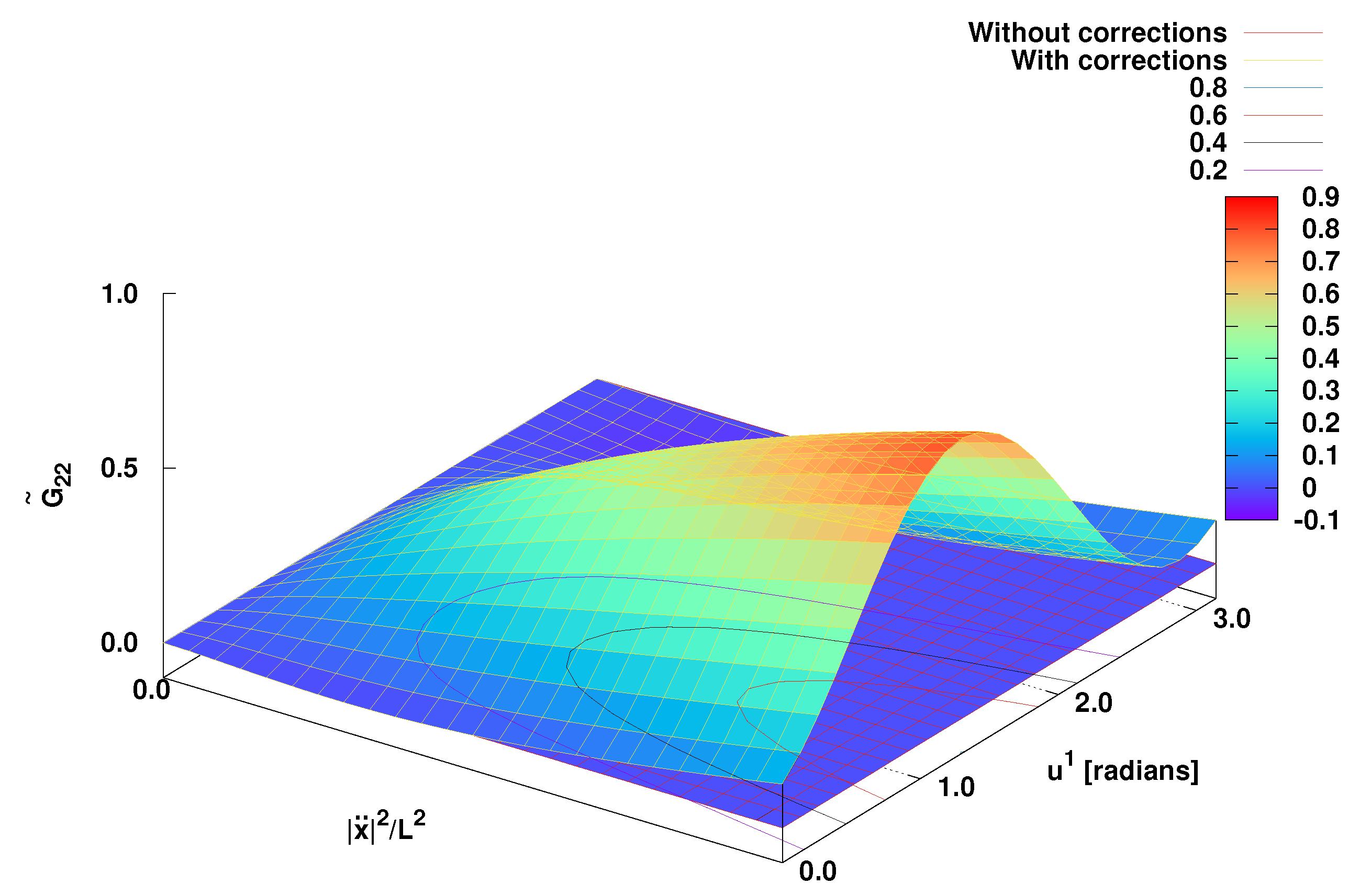
this equation with minimal length contributions including additional curvatures and geometrical structures. They are graphically depicted in Figure 2. It shows the dependence of on inclination and . The latter is normalized to . At vanishing and/or , as in Einstein’s classical GR, there is no dependence on the inclination .
The entire dependence of on and is depicted in Figure 2. Near the equator, the value of comes closer to the value of classical Ricci scalar R. One can roughly estimate that while minimal length correction is positive, at , it’s negative, at . This rich structure is to be discovered in future studies.
7. Deformed Einstein tensor
The Einstein tensor is constructed as
and the deformed Einstein tensor will be
By substituting , , and as given in Eqs. (41), (15), and (44), respectively, into Eq. (47), we get
where the indices and of Ricci scalar have replaced by dummy indices and , respectively, and take as a common factor,
where , take and as common factors,
At , the undeformed is obviously fully retrieved from Eq. (50). At finite , the resulting spacetime curvature seems to have more structures than that of the Einstein’s classical tensor . Accordingly, additional sources of gravity are likely emerging. Their nature shall be characterized elsewhere.
For a sphere surface (two-dimensional manifold) with radius , Eq. (50) gives
Accordingly, a comparison between and is depicted in Figure 3. a sphere surface with radius .
In freely falling frames, in which the covariant derivative of tensor is the same for all observers, and the affine connection is vanishing so that the covariant derivative of deformed Einstein tensor Eq. (50) will be
where in general relativity. In the flat space-time, the covariant derivative is a partial derivative, then Eq. (54) becomes
where see Appendix A. In free falling frame, , then
where . Eq. (59) is valid for flat or curved space-time therefore, the divergence of deformed Einstein tensor is vanishing.
The central assumption of general relativity is that the divergence of vanishes as that of the energy–momentum tensor , that is and . This means that extending the spacetime curvature preserves the central assumption of GR.
8. Summary and Conclusion
As prescribed in loop quantum gravity, doubly–special relativity, string theory, and noncommutative geometry, gravitational impacts could be embedded in the generalized noncommutative Heisenberg algebra. The minimal length correction to the metric tensor could be determined by the extended coordinates (. By equating the line element in the eight-dimensional manifold and the deformed line element in the four-dimensional manifold , the minimal length-induced correction to the metric tensor is determined. With this extension of manifold and minimal length correction, we have been able to extend the affine connection on the Riemann manifold and thereby suggesting minimal length-induced corrections to the Riemann and Ricci curvature tensors and Ricci scalar. Accordingly, we have constructed a deformed version of the Einstein tensor.
In differential geometry, the covariant derivative of Einstein tensor used to describes the spacetime curvature due to the presence of the energy–momentum tensor , the physical quantity expressing density and flux of energy and momentum in curved spacetime, vanishes. We have proved that the covariant derivative of the Einstein tensor with minimal length–induced corrections vanishes, as well. Thus, the deformed spacetime curvature presented in the present script seems to fulfil the entire assumptions of the Einstein’s theory of general relativity, on one hand. On the other hand, the deformation of the spacetime curvature adds additional curvatures and geometric structures and thereby might suggest a generalization of the energy–momentum tensor , which will be discussed in a future research.
Author Contributions
Conceptualization, Abdel Nasser Tawfik; Formal analysis, Fady Farouk, Abdel Nasser Tawfik and Muhammad Abdulghaffar; Methodology, Abdel Nasser Tawfik; Project administration, Muhammad Abdulghaffar; Resources, Fady Farouk; Software, Fady Farouk; Supervision, Fawzy Tarabia and Muhammad Abdulghaffar; Visualization, Fady Farouk; Writing – original draft, Fady Farouk and Abdel Nasser Tawfik; Writing – review & editing, Fawzy Tarabia and Muhammad Abdulghaffar.
Appendix A. The derivative of x ¨ μ with respect to the space-time coordinates
The derivative of with respect to the space-time coordinates can be expressed as
By using the commutation property of partial derivatives,
where [46]. Also, the same argument can be used for ,
References
- Isham, C.J. Prima facie questions in quantum gravity. Canonical Gravity: From Classical to Quantum: Proceedings of the 117th WE Heraeus Seminar Held at Bad Honnef, Germany, 13–17 September 1993. Springer, 2005, pp. 1–21. 13–17 September.
- Bosso, P. On the quasi-position representation in theories with a minimal length. Classical and Quantum Gravity 2021, 38, 075021. [Google Scholar] [CrossRef]
- Bosso, P.; Obregón, O. Minimal length effects on quantum cosmology and quantum black hole models. Classical and Quantum Gravity 2020, 37, 045003. [Google Scholar] [CrossRef]
- Capozziello, S.; Lambiase, G.; Scarpetta, G. Generalized uncertainty principle from quantum geometry. arXiv preprint gr-qc/9910017 1999.
- Adler, R.J.; Santiago, D.I. On gravity and the uncertainty principle. Modern Physics Letters A 1999, 14, 1371–1381. [Google Scholar] [CrossRef]
- Scardigli, F. Generalized uncertainty principle in quantum gravity from micro-black hole gedanken experiment. Physics Letters B 1999, 452, 39–44. [Google Scholar] [CrossRef]
- Kempf, A.; Mangano, G.; Mann, R.B. Hilbert space representation of the minimal length uncertainty relation. Physical Review D 1995, 52, 1108. [Google Scholar] [CrossRef]
- Maggiore, M. A generalized uncertainty principle in quantum gravity. Physics Letters B 1993, 304, 65–69. [Google Scholar] [CrossRef]
- Konishi, K.; Paffuti, G.; Provero, P. Minimum physical length and the generalized uncertainty principle in string theory. Physics Letters B 1990, 234, 276–284. [Google Scholar] [CrossRef]
- Karolyhazy, F. Gravitation and quantum mechanics of macroscopic objects. Il Nuovo Cimento A (1965-1970) 1966, 42, 390–402. [Google Scholar] [CrossRef]
- Mead, C.A. Possible connection between gravitation and fundamental length. Physical Review 1964, 135, B849. [Google Scholar] [CrossRef]
- Yang, C.N. On quantized space-time. Physical Review 1947, 72, 874. [Google Scholar] [CrossRef]
- Snyder, H.S. Quantized space-time. Physical Review 1947, 71, 38. [Google Scholar] [CrossRef]
- Saridakis, E.; Lazkoz, R.; Salzano, V.; Moniz, P.; Capozziello, S.; Jiménez, J.; De Laurentis, M.; Olmo, G. Modified Gravity and Cosmology: An Update by the CANTATA Network; Springer International Publishing, 2021.
- Farag Ali, A.; Das, S.; Vagenas, E.C. The generalized uncertainty principle and quantum gravity phenomenology. The Twelfth Marcel Grossmann Meeting: On Recent Developments in Theoretical and Experimental General Relativity, Astrophysics and Relativistic Field Theories (In 3 Volumes). World Scientific, 2012, pp. 2407–2409.
- Bosso, P. Generalized uncertainty principle and quantum gravity phenomenology; University of Lethbridge (Canada), 2017.
- Garay, L.J. Quantum gravity and minimum length. International Journal of Modern Physics A 1995, 10, 145–165. [Google Scholar] [CrossRef]
- Tawfik, A.; Diab, A. Generalized uncertainty principle: Approaches and applications. International Journal of Modern Physics D 2014, 23, 1430025. [Google Scholar] [CrossRef]
- Kempf, A. Uncertainty relation in quantum mechanics with quantum group symmetry. Journal of Mathematical Physics 1994, 35, 4483–4496. [Google Scholar] [CrossRef]
- Sonego, S. Is there a space-time geometry? Phys. Lett. A 1995, 208, 1–7. [Google Scholar] [CrossRef]
- Farouk, F.T.; Tawfik, A.N.; Tarabia, F.S.; Maher, M. On Possible Minimal Length Deformation of Metric Tensor and Affine Connection. In progress 2022. [Google Scholar]
- Tawfik, A.N.; Diab, A.M. A review of the generalized uncertainty principle. Reports on Progress in Physics 2015, 78, 126001. [Google Scholar] [CrossRef]
- Tawfik, A.N.; Farouk, F.T.; Tarabia, F.S.; Maher, M., Minimal length discretization and properties of modified metric tensor and geodesics, The Sixteenth Marcel Grossmann Meeting. In The Sixteenth Marcel Grossmann Meeting; pp. 4074–4081, [https://www.worldscientific.com/doi/pdf/10.1142/9789811269776_0339]. [CrossRef]
- Tawfik, A.N.; Diab, A.M.; Shenawy, S.; El Dahab, E.A. Consequences of minimal length discretization on line element, metric tensor, and geodesic equation. Astronomische Nachrichten 2021, 342, 54–57. [Google Scholar] [CrossRef]
- Kempf, A.; Mangano, G.; Mann, R.B. Hilbert space representation of the minimal length uncertainty relation. Phys. Rev. D 1995, 52, 1108–1118. [Google Scholar] [CrossRef]
- Bushev, P.; Bourhill, J.; Goryachev, M.; Kukharchyk, N.; Ivanov, E.; Galliou, S.; Tobar, M.; Danilishin, S. Testing the generalized uncertainty principle with macroscopic mechanical oscillators and pendulums. Physical Review D 2019, 100, 066020. [Google Scholar] [CrossRef]
- Abbott, B.P.; others. GW170817: Observation of Gravitational Waves from a Binary Neutron Star Inspiral. Phys. Rev. Lett. 2017, arXiv:gr-qc/1710.05832]119, 161101. [CrossRef] [PubMed]
- Diab, A.M.; Tawfik, A.N. A Possible Solution of the Cosmological Constant Problem based on Minimal Length Uncertainty and GW170817 and PLANCK Observations 2020. [arXiv:physics.gen-ph/2005.03999]. arXiv:physics.gen-ph/2005.03999].
- Tawfik, A.N.; Diab, A.M. Generalized Uncertainty Principle: Approaches and Applications. Int. J. Mod. Phys. D 2014, arXiv:gr-qc/1410.0206]23, 1430025. [Google Scholar] [CrossRef]
- Tawfik, A.N.; Diab, A.M. Review on Generalized Uncertainty Principle. Rept. Prog. Phys. 2015, arXiv:physics.gen-ph/1509.02436]78, 126001. [Google Scholar] [CrossRef] [PubMed]
- Snyder, H.S. Quantized space-time. Phys. Rev. 1947, 71, 38–41. [Google Scholar] [CrossRef]
- Mead, C.A. Observable Consequences of Fundamental-Length Hypotheses. Phys. Rev. 1966, 143, 990–1005. [Google Scholar] [CrossRef]
- Benczik, S.; Chang, L.N.; Minic, D.; Okamura, N.; Rayyan, S.; Takeuchi, T. Short distance versus long distance physics: The Classical limit of the minimal length uncertainty relation. Phys. Rev. D 2002, 66, 026003. [Google Scholar] [CrossRef]
- Kober, M. Gauge Theories under Incorporation of a Generalized Uncertainty Principle. Phys. Rev. D 2010, arXiv:physics.gen-ph/1008.0154]82, 085017. [Google Scholar] [CrossRef]
- Wang, B.Q.; Long, C.Y.; Long, Z.W.; Xu, T. Solutions of the Schrödinger equation under topological defects space-times and generalized uncertainty principle. Eur. Phys. J. Plus 2016, 131, 378. [Google Scholar] [CrossRef]
- Sprenger, M.; Nicolini, P.; Bleicher, M. Physics on the smallest scales: an introduction to minimal length phenomenology. European Journal of Physics 2012, 33, 853. [Google Scholar] [CrossRef]
- Brandt, H. Erratum to: Maximal proper acceleration relative to the vacuum. Lettere al Nuovo Cimento (1971-1985) 1984, 39, 192–192. [Google Scholar] [CrossRef]
- Caianiello, E.R. Some Remarks on Quantum Mechanics and Relativity. Lett. Nuovo Cim. 1980, 27, 89. [Google Scholar] [CrossRef]
- Caianiello, E.R.; Feoli, A.; Gasperini, M.; Scarpetta, G. Quantum Corrections to the Space-time Metric From Geometric Phase Space Quantization. Int. J. Theor. Phys. 1990, 29, 131. [Google Scholar] [CrossRef]
- Caianiello, E.R.; Gasperini, M.; Scarpetta, G. Phenomenological Consequences of a Geometric Model With Limited Proper Acceleration. Nuovo Cim. B 1990, 105, 259. [Google Scholar] [CrossRef]
- Cainiello, E.R.; Gasperini, M.; Scarpetta, G. Inflation and singularity prevention in a model for extended-object-dominated cosmology. Class. Quant. Grav. 1991, 8, 659–666. [Google Scholar] [CrossRef]
- Brandt, H.E. Riemann curvature scalar of space-time tangent bundle. Found. Phys. Lett. 1992, 5, 43. [Google Scholar] [CrossRef]
- Brandt, H.E. Structure of space-time tangent bundle. Found. Phys. Lett. 1991, 4, 523. [Google Scholar] [CrossRef]
- Carroll, S.M. Spacetime and Geometry; Cambridge University Press, 2019.
- Misner, C.W.; Thorne, K.S.; Wheeler, J.A. Gravitation; Macmillan Publishers, 1973.
- Schutz, B. A first course in general relativity; Cambridge university press, 2009.
Figure 1.
Coefficients of the Riemann and Ricci curvature tensors in sphere surface with unity radius. The coefficients of and vary with and in units of .
Figure 1.
Coefficients of the Riemann and Ricci curvature tensors in sphere surface with unity radius. The coefficients of and vary with and in units of .
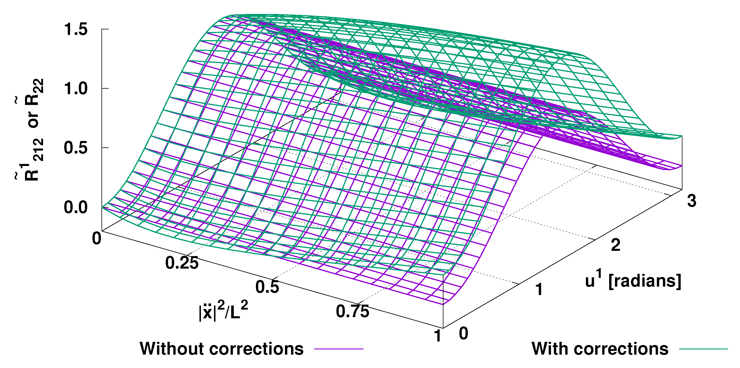
Figure 2.
In a sphere surface with a unity radius, the panel shows how varies with varying and .
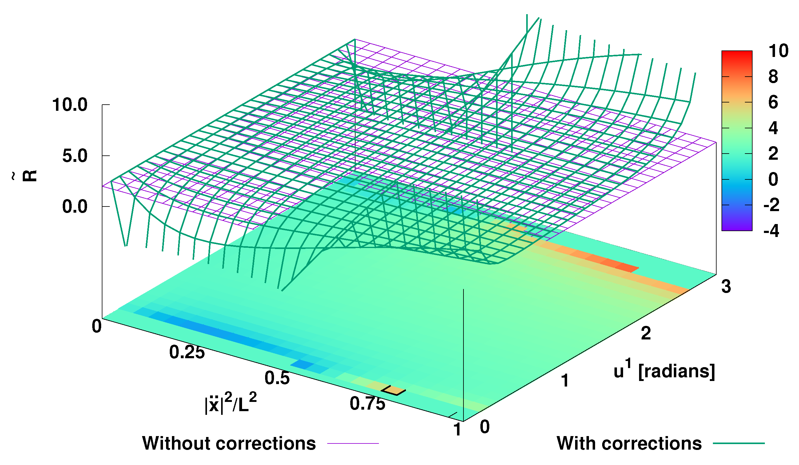
Figure 3.
In a sphere surface with radius , the panel presents –plot of varies with varying and .
Disclaimer/Publisher’s Note: The statements, opinions and data contained in all publications are solely those of the individual author(s) and contributor(s) and not of MDPI and/or the editor(s). MDPI and/or the editor(s) disclaim responsibility for any injury to people or property resulting from any ideas, methods, instructions or products referred to in the content. |
© 2023 by the authors. Licensee MDPI, Basel, Switzerland. This article is an open access article distributed under the terms and conditions of the Creative Commons Attribution (CC BY) license (http://creativecommons.org/licenses/by/4.0/).
Copyright: This open access article is published under a Creative Commons CC BY 4.0 license, which permit the free download, distribution, and reuse, provided that the author and preprint are cited in any reuse.


