Rlc Electrical Modelling of Black Hole and Early Universe. Generalization of Boltzmann’s Constant in Curved Space-Time

1. RC electrical model for a black hole

If considering electric charge and mass as fundamental properties of matter.

From the point of view of electric charge, we know that a capacitor stores electrical energy and we can represent it as an RC circuit.

Analogously, from the mass point of view, we can consider a black hole as a capacitor that stores gravitational potential energy.

Continuing with the analogy, the space-time that surrounds a black hole can be represented as the inductance L.

from this simple conceptual idea was born RLC electrical modelling of black hole and early universe.

RC electrical model for a Black Hole:

Here we put forward the hypothesis of a black hole growth in analogy to an RC electrical circuit that grows according to a constant Tau being defined as:

$$\tau =RC$$

(1)

First, we will consider the total mass of a black hole to consist of the sum of baryonic mass and dark matter mass (Equation (2)), considering dark matter as an imaginary number.

$$M=m-i\delta$$

(2)

where M is the total mass of a black hole, m is the baryonic mass; $\delta$ corresponds to dark matter and I is the irrational number $\sqrt{-1}$. This equation is in analogy to impedance of an RC circuit.

$$Z=R-i{X}_c$$

(3)

where z represents impedance; R represents resistance and Xc represents reactance.

If proper accelerations for the masses are introduced in equation (2) we obtain the following:

$$F=f-i\phi$$

(4)

where F is the total force, f is the force associated to baryonic mass, and i$\phi$ is the force associated to dark mass. In analogy to a phasor diagram for an RC circuit, in which the reactance phasor lags the resistance phasor R by $\frac{\pi }{2}$, we can represent the two forces associated to barionic matter and dark matter as two orthogonal vectors (Figure 1).

Vector diagram of forces in a black hole for circular motion with constant acceleration:

Figure 1. Vector representation of the forces in a black hole. Fc = f, represents the force towards the interior of the black hole generated by the mass m and Ft = -iφ, is a tangential force that retards Fc by 90 degrees, generated by the mass δ.

Figure 1. Vector representation of the forces in a black hole. Fc = f, represents the force towards the interior of the black hole generated by the mass m and Ft = -iφ, is a tangential force that retards Fc by 90 degrees, generated by the mass δ.

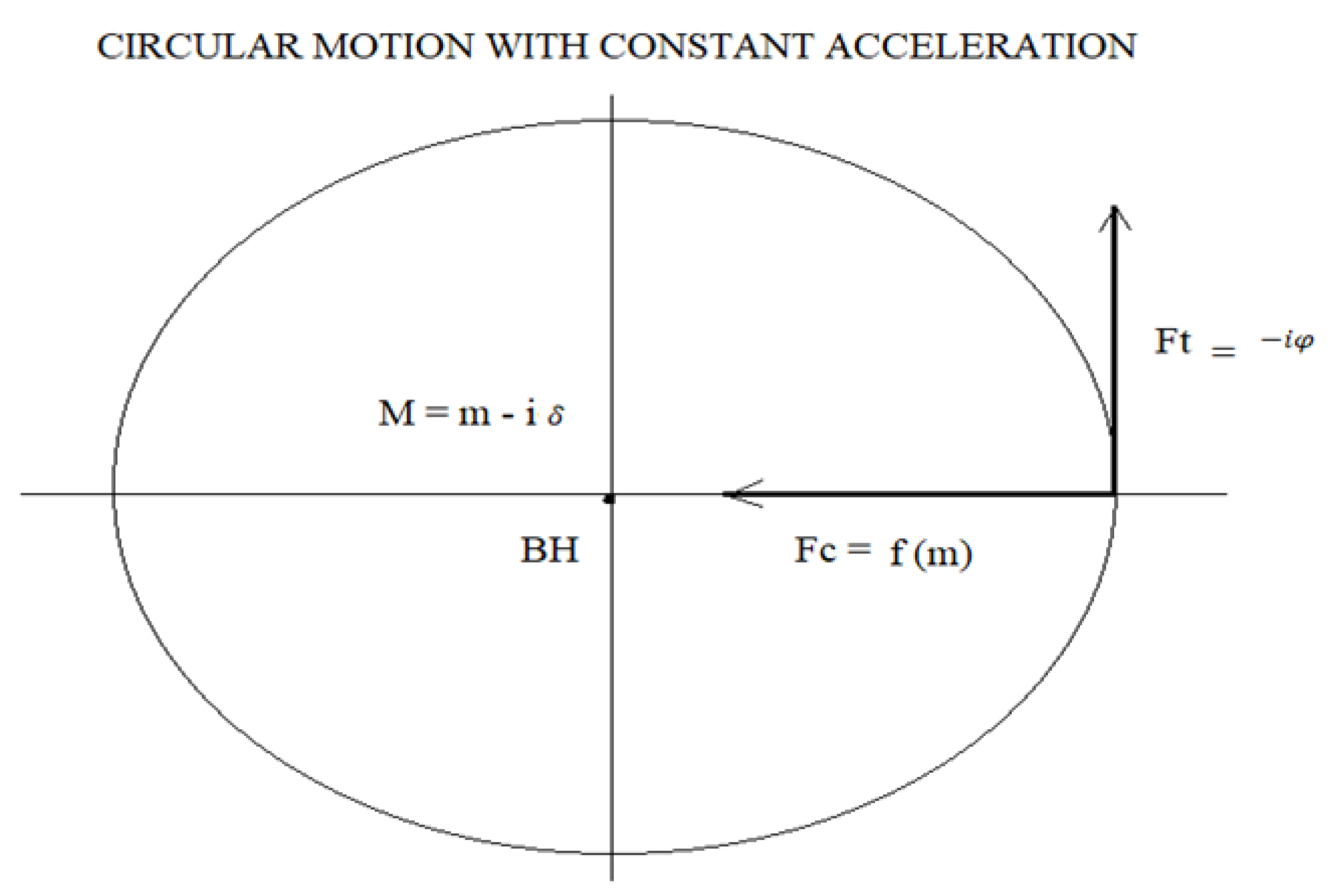
taking into account Newton’s equation of universal gravitation:

F = - (G M1 M2)/r²

The sign (-) of the equation means that the force Fc is at 180 degrees with respect to the resistance R and the force Ft is also at 180 degrees from the reactance Xc.

It is important to make clear the physical interpretation of the imaginary mass, it is simply telling us that the force Fc due to the mass m delays the force ft by 90 degrees, due to the mass δ, that delay is represented by the imaginary number i. Later we will determine that the mass δ, is the result of v > c inside a black hole.

Where v is the speed of a massless particle and c is the speed of light in a vacuum.

Figure 1 is represented for a circular motion with constant acceleration simply because the tangential velocity of a particle is proportional to the radius from the centre of the black hole multiplied by the average angular frequency.

Vt = r ω

The contribution of (Ft, Vt) is what makes the speed of the galaxy remain constant as the radius of the galaxy grows.

Where Vt represents the tangential velocity of a galaxy, r is the radius from the galaxy, and ω is the average angular velocity of the rotation of the galaxy.

Circular motion with constant acceleration tells us that the mass input into a black hole is negligible with respect to the black hole’s own mass.

The growth of a black hole according to the tau constant is an intrinsic property of a black hole and is independent of the amount of matter that enters a black hole.

To calculate the total energy associated to the black hole, we can introduce its total mass (Equation (2)) into:

$$E^2=c^2{p}^2+c^4{M}^2$$

(5)

where E is energy; c represents the speed of light and m represents the mass. This lead to:

$$E^2=c^2{p}^2+\left(m^2-{\delta }^2\right)c^4-2im\delta c^4.$$

(6)

We can assume that during the big bang inflation phase baryonic matter was overrepresented compared to dark matter together with an infinitesimal momentum, which would give us from Equation (6) the following:

$$E^2=-{\delta }^2{c}^4 ; E=(+/-)\delta c^{2}i$$

(7)

As expected, this result corresponds to the total energy of the universe at the big bang if we consider it to be made of dark matter represented as a reactance in an RC circuit.

The positive value of E is determined by matter, there is no antimatter inside a black hole.

If we consider charge as a fundamental property of matter, $E=(+)\delta c^{2}i$, represents the amount of relativistic dark matter inside the black hole at the time of disintegration.

If we consider mass as a fundamental property of matter, $E=(-)\delta c^2$, represents the amount of relativistic dark matter inside a black hole, which exerts a repulsive gravitational force at the moment of disintegration. This repulsive gravitational force is what generates the dark energy after the Big Bang.

At time T0, when the black hole disintegrates and the Big Bang occurs, roughly all matter was dark matter.

We could also consider a universe at infinity proper time in which baryonic matter is dominant over dark matter, which would transform equation (6) back into equation (5) but with baryonic matter.

$$E^2=c^2{p}^2+m^2{c}^4.$$

(8)

2. RLC Electrical Model of the Universe

We will analyse the Dirac delta function &(t).

&(t) = {∞, t = 0} ^ {0, t ≠ 0}

If we perform the Fourier transform of the function &(t) and analyse the amplitude spectrum, we observe that the frequency content is infinite.

If we perform the Fourier transform of the function &(t) and analyse the phase spectrum, we observe that the phase spectrum is zero for all frequencies.

We say that it is a non-causal zero phase system.

The most important thing to emphasize in this system is that an infinite impulse has an infinite frequency content.

When we work in seismic prospecting looking for gas or oil, using explosives, the detonations produce an energy peak that generates a frequency spectrum that propagates in the layers of the earth. The energy produced in the detonation is not instantly transferred to the ground, a time delay occurs, it is said to be causal system of minimum phase.

In analogy, we are going to suppose that the Big Bang also behaves like a causal system of minimum phase.

Here we put forward the hypothesis that the big bang is the convolution of the energy released by disintegration of the black hole with the space-time surrounding the black hole, being defined as:

$$( m-i\delta ) * Ɛ$$

(9)

where $m-i\delta ,$ is the total mass of a black hole, Ɛ is the space-time surrounding the black hole and * is the convolution symbol.

Equation (9) can be simplified and considered analogous to an RLC circuit.

where RC represents a black hole and L represents the space-time around a black hole

$$RC=m-i\delta$$

(10)

$$L=ℇ$$

(11)

the resolution of the quadratic equation of the RLC circuit will determine how space-time will expand after the Big Bang and the bandwidth of the equation will give us the spectrum of gravitational waves that originated during the Big Bang.

3. Cosmic Inflation

From the following equation:

$${\mathrm{d}\mathrm{s}}^2=-\left(1-\left(\frac{2\mathrm{M}\mathrm{G}}{{\mathrm{R}\mathrm{c}}^2}\right)\right){\mathrm{c}}^2{\mathrm{d}\mathrm{t}}^2+\left(1/\left(1–\frac{2\mathrm{M}\mathrm{G}}{{\mathrm{R}\mathrm{c}}^2}\right)\right){\mathrm{d}\mathrm{R}}^2+{\mathrm{R}}^2\mathrm{d}{\mathsf{\theta }}^2+{\mathrm{R}}^2{\mathrm{s}\mathrm{i}\mathrm{n}}^2\mathrm{d}$$

(12)

We will analyse the Schwarzschild solution for a punctual object in which mass and gravity are introduced.

$$Rs=2GM / c², is the Schwarzschild´s radius.$$

(13)

where M is the mass of a black hole, c is the speed of light, and G is the gravitational constant.

if we consider dθ = 0; and dφ = 0; that is, we move in the direction of dR.

(14)

R = Rs, ds = 0, let’s analyse this specific situation.

(15)

Replacing the conditions given in (13), (14) and (15) in Equation (12), we have:

(dR / dt) ² = v² = c² (1 - (2MG/Rc²) ²

R = Rs, v = 0; ds² = 0; Rs is the Schwarzschild´s radius.

(16)

R > Rs, v < c; ds < 0, time type trajectory.

(17)

R < Rs, v > c; ds > 0, space type trajectory.

(18)

Condition (18) is very important because to the extent that R < Rs, v > c is fulfilled, it is precisely this speed difference that generates the imaginary mass in a black hole given by $-i\delta .$

Planck length equation:

$$Lp = \surd (h G /c ³)$$

(19)

where h is Planck’s constant, G is the gravitational constant, and c is the speed of light.

If we consider condition (18) and Equation (19), to the extent that R < Rs and v > c, are fulfilled, we deduce that the Planck length decreases in value.

We define the following:

Lpɛ = Lp = 1.616199 10⁻³⁵ m; electromagnetic Planck length.

Lpɢ = gravitational Planck length.

Always holds:

Lpɢ < Lpɛ

Here we put forward the hypothesis that cosmic inflation is the expansion of space-time that is given by Lpɢ that tends to reach its normal value Lpɛ after a black hole disintegrates.

If we consider the Planck length Lpɛ, the minimum length of space-time, like a spring and due to the action of v > c (300,000 km/s), this length decreases in values of Lpɢ, that is, Lpɢ < Lpɛ, allowing us to imagine the immense forces involved in compressing space-time of length Lpɛ into smaller values of space-time Lpɢ. The immense energy stored and released in the spring of length Lpɢ, to recover its initial length Lpɛ, is the cause of the exponential expansion of space-time in the first moments of the Big Bang.

At time T0, when the black hole disintegrates and the Big Bang occurs, roughly all matter was dark matter, relativistic dark matter.

4. Generalization of the Boltzmann’s Constant for Curved Space-Time

Equation of state of an ideal gas as a function of the Boltzmann constant.

$$P V=N KB T$$

(20)

where, P is the absolute pressure, V is the volume, N is the number of particles, KB is Boltzmann’s constant, and T is the absolute temperature.

Boltzmann’s constant is defined for 1 mole of carbon 12 and corresponds to 6.0221 10²³ atoms.

Equation (20) applies for atoms, molecules and for normal conditions of pressure, volume and temperature.

We will analyse what happens with equation (20) when we work in a degenerate state of matter.

We will consider an ideal neutron star, only for neutrons.

We will analyse the condition:

$$(P V) / T = N KB = constant$$

(21)

This condition tells us that the number of particles remains constant, under normal conditions of pressure, volume and temperature

However, in an ideal neutron star, the smallest units of particles are neutrons and not atoms.

This leads us to suppose that number of neutrons would fit in the volume of a carbon 12 atom, this amount can be represented by the symbol Dn.

In an ideal neutron star,

$$\left(\mathrm{P}\mathrm{V}\right)/\mathrm{T}=\mathrm{D}\mathrm{n} \mathrm{N} \mathrm{K}\mathrm{B}$$

(22)

where Dn represents the number of neutrons in a carbon 12 atom.

However, Equation (22) is not constant, with respect to equation (21), the number of particles increased by a factor Dn, to make it constant again, I must divide it by the factor Dn.

$$(P V) / T=Dn N KB / Dn$$

(23)

$$(P V) / T=N´ KB´=constant$$

(24)

where N’ = (Dn N), is the new number of particles if we take neutrons into account and not atoms as the fundamental unit.

where KB’ = (KB / Dn), is the new Boltzmann´s constant if we take neutrons into account and not atoms as the fundamental unit.

We can say that Equation (21) is equal to Equation (24), equal to a constant

Generalizing, it is the state in which matter is found that will determine Boltzmann’s constant.

A white dwarf star a will have a Boltzmann´s constant KBe, a neutron star will have a Boltzmann´s constant KBn, and a black hole will have a Boltzmann´s constant KBq.

There is a Boltzmann´s constant KB that we all know for normal conditions of pressure, volume and temperature, for a flat space-time.

There is an effective Boltzmann´s constant, which will depend on the state of matter, for curved space-time.

The theory of general relativity tells us that in the presence of mass or energy space-time curves but it does not tell us how to quantify the curvature of space-time.

Here we put forward the hypothesis that there is an effective Boltzmann´ constant that depends on the state of matter and through the value that the Boltzmann´ constant takes we can measure or quantify the curvature of space-time.

Quantifying space-time, considering the variable Boltzmann constant, is also quantizing gravitational waves and, as with the electromagnetic spectrum, we will determine that there is a spectrum of gravitational waves.

These analogies to represent the gravitational and electromagnetic wave equations are achieved thanks to the ADS/CFT correspondence.

We can determine the equations of electromagnetic and gravitational waves as shown below.

Electromagnetic wave spectrum for flat space-time:

Eε = h x fε

Cε = λε x fε

Eε = h x Cε / λε

Eε = Kʙε x Tε

Kʙɛ = 1.38 10⁻²³ J/K

Gravitational wave spectrum for curved spacetime:

Eɢ = h x fɢ

Cɢ = λɢ x fɢ

Eɢ = h x Cɢ / λɢ

Eɢ = Kʙɢ x Tɢ

Kʙɢ = 1.38 10⁻²³ J/K to 1.78 10⁻⁴³ J/K.

Where the subscript ε means electromagnetic and the subscript ɢ means gravitational.

It can be seen that there is an electromagnetic and a gravitational frequency as well as an electromagnetic and a gravitational temperature.

The maximum curvature of space-time occurs for an effective Boltzmann´s constant of KB = 1.78 10⁻⁴³ J/K, given by the ADS/CFT correspondence in which a black hole is equivalent to the plasma of quarks and gluons to calculate the viscosity of the plasma of quarks and gluons.

Once a black hole is formed and the maximum curvature of space-time is reached, as a black hole grows following the tau growth law analogous to an RC circuit, as v grows fulfilling the relationship v > c, it happens that the gravitational Planck length becomes less than the electromagnetic Planck length, it holds that Lpɢ < Lpɛ.

5. Black Hole’S Radiation

Equation (2) defines the mass of a black hole, as shown below:

$$M=m-i\delta$$

(25)

where M is the total mass of a black hole, m is the baryonic mass; $\delta$ corresponds to dark matter and i is the irrational number $\sqrt{-1}$.

Also, here we put forward the hypothesis of a black hole growth in analogy to an RC electrical circuit that grows according to a constant Tau being defined as:

$$\tau =RC$$

(26)

If we consider the black hole´s radiation that produces pairs of particles and antiparticles at the event horizon.

Here we put forward the hypothesis:

the HR (matter) particle, with frequency ω and energy hω, falls into the black hole and adds to m and δ increasing the mass of the black hole, that is, it adds mass.

This is defined with the assumption that a black hole grows according to the tau constant just like an RC circuit.

The P particle (antimatter), with frequency ω and energy -hω, moves away from the black hole in the form of a gravitational wave.

According to the proposed hypothesis, a black hole always grows, following the curve of the tau constant in analogy to an RC electrical circuit.

For a black hole of 3 solar masses, the stationary frequency would be approximately 2.6 10³ Hz.

6. Application Of The Model And Results

6.1. Additional calculations. Growth of a black hole in analogy to the tau growth curve of an RC circuit

In the ADS/CFT correspondence to calculate the viscosity of quark-gluon plasma, the following assumption is used, a black hole is equivalent to quark-gluon plasma.

We consider the temperature of a black hole equal to the temperature of the quark-gluon plasma, equal to T = 10¹³ K.

Another way of interpreting it is as follows:

When a star collapses, a white dwarf star, a neutron star, or a black hole is formed.

A white dwarf star has a temperature of about 10⁶ K, a neutron star has a temperature of about 10¹¹ K. If we consider that a black hole is a plasma of quarks and gluons, its temperature is expected to be higher than 10¹¹ K.

Hypothesis: the temperature of a black hole is 10¹³ K.

We will make the following approximation:

T = 0.0000000000001τ, T = 10⁻¹³τ

τ = 10²⁶ K

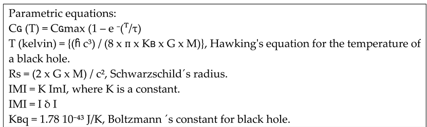
Cɢ(T) = Cɢmax (1 - e⁻(ᵀ/τ))

Cɢ(T) = Cɢmax (1 - e ⁻ ⁰·⁰⁰⁰⁰⁰⁰⁰⁰⁰⁰⁰¹(τ/τ))

Cɢ(T) = Cɢmax (1 - e ⁻ ⁰·⁰⁰⁰⁰⁰⁰⁰⁰⁰⁰⁰⁰¹)

Cɢ(T) = Cɢmax (1 - e ⁻ (¹ / 10¹³)

Cɢ(T) = Cɢmax (1 - 1 / e (¹/ 10¹³))

Cɢ(T) = Cɢmax (1 – 0.9999999999999)

Cɢ(T) = Cɢmax x 10⁻¹³

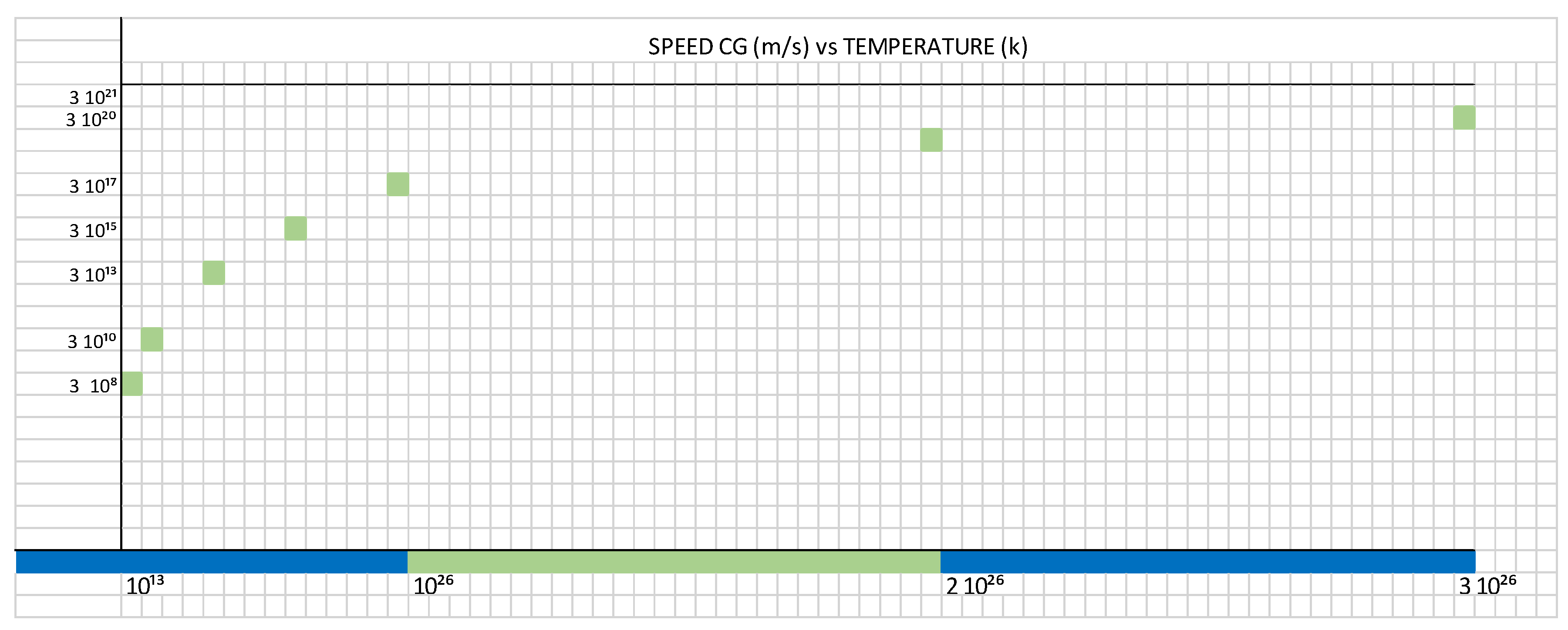
Cɢmax = Cɢ(T) / 10⁻¹³ = 3 10⁸ m/s x 10¹³

Cɢmax ≡ 3 10²¹ m/s.

where T is the absolute temperature, τ represents the growth constant tau, Cɢ = v represents the speed of a massless particle greater than the speed of light and Cɢmax represents the maximum speed that Cɢ can take.

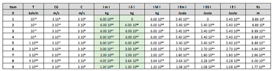
With the following equations we obtain the following graphs, represented by Table 1 and Figure 2:

(a)

In item 1 of the Table 1, for the following parameters, T = 10¹³ K, Cɢ = C = 310⁸ m/s, calculating we get the following values:

m = 6 10³⁰ kg, baryonic mass.

δ = 0, dark matter mass.

M = m = 6 10³⁰ kg

Rs = 8,89 10³ m, Schwarzschild radius.

(b)

In item 9 of the Table 1, for the following parameters, T = 5 10²⁶ K, Cɢ = 3 10²¹ m/s, C = 310⁸ m/s, calculating we get the following values:

m = 1.20 10⁵⁶ kg, baryonic mass.

δ = 1.20 10⁸² kg, dark matter mass.

M = δ = 1.20 10⁸² kg

Rs = 1.77 10²⁹ m, Schwarzschild radius.

(c)

It is important to emphasize, for the time t equal to 5τ, at the moment the disintegration of the black hole occurs, the big bang originates, the total baryonic mass of the universe corresponds to m = 10⁵⁶ kg.

(d)

Figure 2 shows the growth of the tau (τ) constant, as a function of speed vs. temperature.

Table 1. Represents values of ImI, baryonic mass; IδI, dark matter mass; IMI, mass of baryonic matter plus the mass of dark matter; IEmI, energy of baryonic matter; IEδI, dark matter energy; IEI, Sum of the energy of baryonic matter plus the energy of dark matter and Rs, Schwarzschild´s radius, as a function of, c, speed of light; Cɢ, speed greater than the speed of light; T, temperature in Kelvin; using the parametric equations.

Table 1. Represents values of ImI, baryonic mass; IδI, dark matter mass; IMI, mass of baryonic matter plus the mass of dark matter; IEmI, energy of baryonic matter; IEδI, dark matter energy; IEI, Sum of the energy of baryonic matter plus the energy of dark matter and Rs, Schwarzschild´s radius, as a function of, c, speed of light; Cɢ, speed greater than the speed of light; T, temperature in Kelvin; using the parametric equations.

Figure 2. Represents the variation of speed Cɢ, as a function of temperature T, inside a black hole.

Figure 2. Represents the variation of speed Cɢ, as a function of temperature T, inside a black hole.

6.2. Calculation of the amount of dark matter that exists in the Milky Way

Mass and Schwarzschild´s radius of the Sagittarius A* black hole:

m = 4.5 10⁶ Ms = 4.5 x 10⁶ x 1.98 10³⁰ kg

Where Ms is the mass of the sun.

m = 8.1 x 10³⁶ kg

Rs = 6 million kilometres

Where Rs is the Schwarzschild´s radius of the Sagittarius A*.

Rs = 6 x 10⁹ m

If we look at Figure 2, for m = 8.1 x 10³⁶ kg and Rs = 6 x 10⁹ m, extrapolating we have approximately that T = 3 10¹⁴ K.

To calculate the speed Cɢ we are going to use the Hawking temperature equation:

T = hc³ / (8ᴨ x KB x G x M)

Where h is Boltzmann’s constant, c is the speed inside a black hole, KB is Boltzmann’s constant, G is the universal constant of gravity, and M is the mass of the black hole.

Substituting the values and calculating the value of C we have:

Cɢ = 10.30 10¹⁰ m/s

If we look at Figure 3, we see that this value corresponds approximately to the calculated value.

With the value of Cɢ we calculate δ and M:

E = M C²

Where E is energy, M is mass, and C is the speed of light.

Eɢ = M Cɢ

Eɢ = K M C²

Cɢ ² = k C²

Where K is a constant.

Calculation of the constant K:

C = 3 10⁸ m/s,

Cɢ = 10.30 10¹⁰ m/s,

M = 8.1 10³⁶ kg

E = 8.1 10³⁶ kg x 9 10¹⁶ m²/s²

Eɢ = 8.1 10³⁶ x (10.30 10¹⁰) ² = 8.1 10³⁶ x 106 10²⁰

Eɢ = (106 / 9) 10⁴ x 8.1 10³⁶ x 9 10¹⁶

Eɢ = K E

K = 11.77 10⁴

Calculation of the total mass M:

M = K m

M = (11.77 10⁴) x (8.1 10³⁶ kg)

M = 9.54 10⁴¹ kg, Total mass of black hole Sagittarius A*

m = 8.1 x 10³⁶ kg, total baryonic mass inside the black hole Sagittarius A*

Calculation of the mass of dark matter δ:

M = δ

δ = 9.54 10⁴¹ kg, total dark matter inside the black hole Sagittarius A*

Calculation of the ratio of the mass of dark matter and the mass of the Milky Way

Mvl = 1.7 10⁴¹ kg, mass of the milky way

δ = 9.54 10⁴¹ kg, total dark matter inside the black hole Sagittarius A*

δ / Mvl = (9.54 10⁴¹ kg / 1.7 10⁴¹ kg)

δ / Mvl = 5.61, ratio of the mass of dark matter and the mass of the Milky Way

δ = 5.61 Mvl

The total dark matter δ is 5.61 times greater than the measured amount of baryonic mass of the Milky Way Mvl.

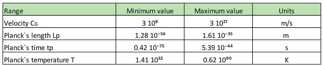
6.3. Calculation of the variations of the Planck length, Planck time and Planck temperature as a consequence of the fact that the velocity v varies from 310⁸ m/s to 3 10²¹ m/s

We define the following:

$$C\epsilon = 310⁸ m/s$$

(27)

$$Cɢmax=3 10²¹ m/s$$

(28)

Cε < Cɢ < Cɢmax

where ε stands for electromagnetic, ɢ stands for gravitational, and max stands for maximum.

Planck´s length equation:

$$Lp = \surd (h G / C ³)$$

(29)

Planck´s time equation:

$$tp = \surd (h G / C ⁵)$$

(30)

Planck’s temperature equation:

$$Tp = \surd \{h C⁵ / (G K{B}^2\left)\right\}$$

(31)

where Lp represents the Planck´s length, tp represents the Planck´s time, and Tp represents the Planck´s temperature.

where h stands for Planck’s constant, C for the speed of light, G for the universal constant of gravity, and KB for Boltzmann’s constant.

Substituting the values of (27) and (28) in equations (29), (30) and (31) we obtain:

Electromagnetic Planck constants:

Cɛ = 3 x 10⁸ m/s

Lpɛ = 1.61 10⁻³⁵ m

tpɛ = 5.39 10⁻⁴⁴ s

Tpɛ = 1.41 10³² K

Gravitational Planck constants:

Cɢ = 3 x 10⁸ m/s to 3 x 10²¹ m/s

Lp = 1.61 10⁻³⁵ m to 1.28 10⁻⁵⁴ m

tp = 5.39 10⁻⁴⁴ s to 0.426 10⁻⁷⁵ s

Tp = 1.41 10³² K to 0.62 10⁹⁰ K

Table 2. we represent the range of variation of the velocity C, the Planck´s length, the Planck´s time and the Planck´s temperature.

Table 2. we represent the range of variation of the velocity C, the Planck´s length, the Planck´s time and the Planck´s temperature.

6.4. The observation of the 1919 solar eclipse in Brazil and Africa provided the first experimental proof of the validity of Albert Einstein’s theory of relativity. We will calculate the Boltzmann constant for the sun and show how it adjusts to the deviation found.

No solar eclipse has had as much impact in the history of science as that of May 29, 1919, photographed and analysed at the same time by two teams of British astronomers. One of them was sent to the city of Sobral, Brazil, in the interior of Ceará; the other to the island of Principe, then a Portuguese territory off the coast of West Africa. The goal was to see if the path of starlight would deviate when passing through a region with a strong gravitational field, in this case the surroundings of the Sun, and by how much this change would be if the phenomenon was measured.

Einstein introduced the idea that gravity was not a force exchanged between matter, as Newton said, but a kind of secondary effect of a property of energy: that of deforming space-time and everything that propagates over it, including waves like light. “For Newton, space was flat. For Einstein, with general relativity, it curves near bodies with great energy or mass”, comments physicist George Matsas, from the Institute of Theoretical Physics of the São Paulo State University (IFT-Unesp). With curved space-time, Einstein’s calculated value of light deflection nearly doubled, reaching 1.75 arcseconds.

The greatest weight should be given to those obtained with the 4-inch lens in Sobral. The result was a deflection of 1.61 arc seconds, with a margin of error of 0.30 arc seconds, slightly less than Einstein’s prediction.

Demonstration:

(i)

Let us calculate the Boltzmann´s constant for the Sun, Kʙs, curved spacetime.

Hawking’s temperature equation:

$$Kʙs = (h x c³) / (8 x \pi x Ts x G x Ms)$$

where Kʙs is the Boltzmann constant for the sun, Ts is the temperature of the sun’s core, G is the universal constant of gravity, and Ms is the mass of the sun.

Kʙs = (6.62 10⁻³⁴ x 27 10²⁴) / (8 x 3.14 x 1.5 10⁷ x 6.67 10⁻¹¹ x 1.98 10³⁰)

Kʙs = 3.59 10⁻³⁷ J/K, Boltzmann’s constant of the sun.

We use the following equation:

Es = Kʙs x Ts

Es = 3.59 10⁻³⁷ x 1.5 10⁷

Es = 5.38 10⁻³⁰ J/K

We use the following equation:

Es = h x fs

fs = Es / h

fs = 5.38 10⁻³⁰ / 6.62 10⁻³⁴ = 0.81 10⁴ = 8.1 10³ Hz

fs = 8.1 10³ Hz

We use the following equation:

c = λs x fs

λs = c / fs

λs = 3 10⁸ / 8.1 10³

λs = 3.7 10⁴ m

We use the following equation:

Degree = λs / 360

Degree =102.77 m

We use the following equation:

Arcsecond = degree / 3600

Arcsecond = 102.77 m / 3600 = 0.0285 m

1.61 arcsecond = 0.0458 m

1 inch = 0.0254 m

4 inch = 0.1016 m

With a 4-inch lens, we can measure the deflection produced by the 1.61 arcsecond curvature of space-time, which was predicted by Albert Einstein’s theory of general relativity, and corresponds to a wavelength λs = 3.7 10⁴ m, a frequency fs = 8.1 10³ Hz, for an effective Boltzmann constant of the sun Kʙs = 3.59 10⁻³⁷ J/K.

(ii)

We will carry out the same calculations for Kʙ = 1.38 10⁻²³ J/K, flat space-time.

Kʙ = 1.38 10⁻²³ J/K

We use the following equation:

E = Kʙ x Ts

E = 1.38 10⁻²³ x 1.5 10⁷

E = 2.07 10⁻¹⁶ J/K

We use the following equation:

E = h x f

f = E / h = 2.07 10⁻¹⁶ / 6.62 10⁻³⁴

f = 3.12 10¹⁷ Hz

We use the following equation:

c = λ x f

λ = c / f

λ = 3 10⁸ / 0.312 10¹⁸

λ = 9.61 10⁻¹⁰ m

We use the following equation:

Degree = λ / 360

Degree = 0.02669 10⁻¹⁰ m

We use the following equation:

Arcsecond = degree / 3600

Arcsecond = 7.41 10⁻¹⁶ m

Using the Boltzmann constant Kʙ = 1.38 10⁻²³ J/K, we cannot correctly predict by mathematical calculations the deflection of light given by Albert Einstein’s general theory of relativity, to be measured in the telescope at Sobral.

Through the example given, we can conclude that the Boltzmann´s constant Kʙs = 3.59 10⁻³⁷ J/K fits the calculations of the deflection of light in curved space-time.

6.5. Dark energy and its relationship with the wave equation of the universe produced by the big bang and the generalization of Boltzmann’s constant for curved space-time.

(a)

Calculation of the wave equation of the universe for the time T0 when the Big Bang occurs:

we will use the Table 1.

Table 1. Represents values of ImI, baryonic mass; IδI, dark matter mass; IMI, mass of baryonic matter plus the mass of dark matter; IEmI, energy of baryonic matter; IEδI, dark matter energy; IEI, Sum of the energy of baryonic matter plus the energy of dark matter and Rs, Schwarzschild’s radius, as a function of, c, speed of light; Cɢ, speed greater than the speed of light; T, temperature in Kelvin; using the parametric equations.

Table 1. Represents values of ImI, baryonic mass; IδI, dark matter mass; IMI, mass of baryonic matter plus the mass of dark matter; IEmI, energy of baryonic matter; IEδI, dark matter energy; IEI, Sum of the energy of baryonic matter plus the energy of dark matter and Rs, Schwarzschild’s radius, as a function of, c, speed of light; Cɢ, speed greater than the speed of light; T, temperature in Kelvin; using the parametric equations.

We are going to consider that at the instant t=0¯, the black hole is about to disintegrate.

Calculation of gravitational waves for a damped parallel RLC circuit (α > ωo).

Initial conditions:

V(0)¯ = 1.08 10⁷³ V, V is equivalent to E

I(0)r = I(0)c = 3 10²¹ A, I is equivalent to C

Calculation of the value of the wavelength lambda λ.

λ = 1.000.000 light years = 10⁶ x 9.46 10¹⁵ m

λ = 9.46 10²¹ m

Calculation of the value of the frequency f:

C = λ x f

f = C / λ

f = 3 10²¹ / 9,46 10²¹

f = 0.317 Hz

Calculation of the value of the angular frequency ω:

ω = 2 ᴨ f

ω = 2.00 rad/s

Calculation of the value of the resistor R:

V (0) = I (0) x R

R = V (0) / I (0) = 1.08 10⁷³ / 3 10²¹

R = 3.60 10⁵¹ Ohms

Calculation of the number of seconds in 380,000 years:

t = 11.81 10¹² s

Let’s consider α = 55 10⁹ ωo

α = 110 10⁹

let’s define:

ω = ωo = 2.00 rad/s; the fundamental frequency is equal to the resonant frequency.

α = 1 / 2RC

Calculation of the value of capacitance C:

C = 1 / 2Rα

C = 1 / (2 x 3.60 10⁵¹ x 110 10⁹)

C = 1.26 10⁻⁶³ F

Calculation of the value of inductance L:

ωo² = 1/LC

L = 1/ (ωo² x C) = 1 / (4 x 1.26 10⁻⁶³)

L = 1.98 10^62 Hy

Calculation of the value of S1:

S1 = -α + √ (α² - ωo²)

S1 = - 1.81 10⁻¹¹

Calculation of the value of S2:

S2 = -α - √ (α² - Wo²)

S2 = -2.19 10¹¹

With these calculated values we have the following equation:

$$V\left(t\right)=A1e^{^}(-1.81 {10}^{-11\mathrm{t}})+A2e^{^}(-2.19x{10}^{11\mathrm{t}})$$

(32)

Calculations of the constant A1 and A2:

First condition V(0):

V(t) = A1 e^ (-1.81 10⁻¹¹ᵗ) + A2 e^ (-2.19 x 10¹¹ᵗ)

V (0) = A1 + A2 = 0

$$A1=-A2$$

(33)

Second condition dV(0) / dt:

V(t) = A1 e^ (-1.81 10⁻¹¹ᵗ) + A2 e^ (-2.19 x 10¹¹ᵗ)

d V(t) / dt = d (A1 e^ (-1.81 10⁻¹¹ᵗ) + A2 e^ (-2.19 x 10¹¹ᵗ))

dV(t)/dt = - 1.81 10⁻¹¹ x A1 x e^-1.81 10⁻¹¹ᵗ - 2.19 10¹¹ x A2 x e^-2.19 10¹¹ᵗ

$$dV\left(0\right)/dt=-1.81 {10}^{-11t}xA1–2.19 {10}^{11t}xA2$$

(34)

Let’s calculate dV(0)/dt = ?

Third condition:

IR + IC + IL = 0; but for t = 0, IL = 0 then it remains

V/R + CdV(t)/dt =0

dV(0)/dt = V/RC

$$dV\left(0\right)/dt=2.38 {10}^{84}$$

(35)

Combining the equations (33), (34) and (35) we obtain the following values for A1 and A2:

A1 = + 1.086 10⁷³

A2 = - 1.086 10⁷³

Substituting the values of A1 and A2 in Equation (32) we obtain the equation of gravitational waves of the Big Bang for the time T0.

$$E\left(t\right)=1.08 {10}^{73}\left\{e^{^}-\left(1.81 {10}^{-11t}\right)\right\}–1.08 {10}^{73}\left\{e^{^}-\left(2.19 {10}^{11t}\right)\right\}+Eo$$

(36)

Where E(t) represents the energy of gravitational waves and E0 represents the energy that corresponds to the temperature of 2.7K.

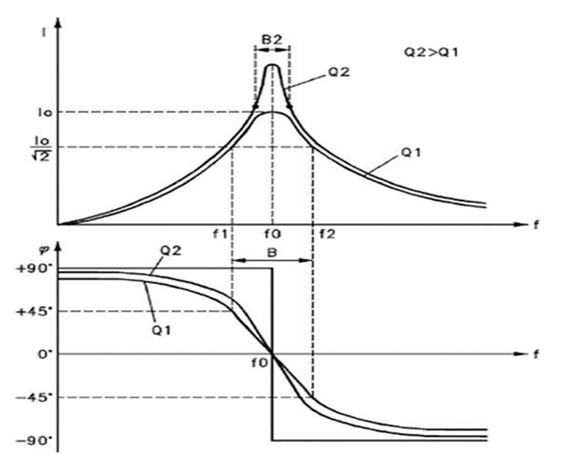
The spectrum of amplitude and phase as a function of frequency (Figure 3) is the Fourier transform from ideal similar Equation (36).

The amplitude spectrum shows us the frequency content as a function of the magnitude.

The phase spectrum shows the frequency content as a function of the angle, but we have to remember by Fourier that the angle is a function of time, therefore a variation of angle implies a variation in displacement and it is precisely this very important characteristic, which we can relate to dark energy.

Figure 3. shows the amplitude spectrum as a function of frequency at the top and the phase spectrum as a function of frequency at the bottom.

Figure 3. shows the amplitude spectrum as a function of frequency at the top and the phase spectrum as a function of frequency at the bottom.

Here we put forward the hypothesis that dark energy is the expansion of space-time that is produced by a spectrum of gravitational waves whose produced frequencies are a function of time, when the disintegration of a black hole (big bang) occurs.

Here we put forward the hypothesis that dark energy is the result of relativistic dark matter that propagates when the black hole disintegrates (Big Bang).

Therefore, dark energy is the result of the combination of the spectrum of gravitational waves whose frequency content is a function of time added to the relativistic dark matter, both propagate with the disintegration of the black hole (Big Bang).

Additional calculations

Calculation of the temperature of the universe for a time t = 380,000 years:

Let’s calculate E (t) for t = 11.81 10^12 s, (380,000 years)

E (t) = 1.08 10⁷³ {e^ - (1.81 10⁻¹¹ᵗ)} – 1.08 10⁷³ {e^ - (2.19 10¹¹ᵗ)}

E (t) = 1.08 10⁷³ {e⁻²¹³}

E (t) = 0.33 10⁻¹⁹ Joules

T = E/KB

T = 2390 k

Approximately the temperature of the cosmic microwave background.

Calculation of the time t for when the universe stabilizes and reaches the temperature of 2.7 K

$$2.7K=3.72 {10}^{-23}J$$

(37)

Substituting (37) in equation (36) we have:

3.72 10⁻²³ = 1.08 10⁷³ e ^ - (1.81 10⁻¹¹ᵗ)

e ^ (1,81 10⁻¹¹ᵗ) = 0.290 10⁹⁶

1.81 10⁻¹¹ᵗ = ln (0.290 10⁹⁶)

t = 1.22 10¹³ s

In that time t the space-time travels the following distance:

e = v x t

Where e is space, v is velocity, and t is time.

e = 3 10²¹ m/s x 1.22 10¹³ s

$$e=3.66 {10}^{34}m$$

(38)

If we calculate the Fourier transform of Equation (32), that is, E (ω).

All the frequencies that make up the frequency spectrum have to travel the distance given by Equation (38), that is, 3.66 10³⁴ m.

Therefore, the influence of the spectrum of gravitational waves in the expansion of space-time will be twice as long, that is, 2.44 10²⁶ s

If we divide by power of 10, logarithmic scale, we have approximately 26 steps.

Let’s calculate the time t today.

t= 4.35 10¹⁷ s, correspond to 17 steps.

(17,5 / 26) × 100 = 67.3%, this is similar to the dark energy content of the universe.

100% - 67.3 = 32.7 %, this is similar to the dark matter content of the universe.

Calculation of the number of seconds in 380,000 years:

$$t = 11.81 10¹² s$$

(39)

Calculation of the number of seconds for when the universe stabilizes and reaches the temperature of 2.7 K

$$t=1.22 10¹³ s$$

(40)

We divide the time t, given by (39) by the time t, in (40), we get:

(11.81 10¹² s / 1.22 10¹³ s) x 100 = 96.72 %

100% - 96,72% = 3.28%, this is similar to the baryonic matter content in the universe.

The true interpretation of this result is the following, the fundamental wavelength that corresponds to λ = 1,000,000 light years, represents the fundamental peak of the CMB sound spectrum, has convolved 96% with the space-time of the universe and still needs to be convolved 4%.

All these calculations are referenced to a time t = 11.81 10¹² s, which correspond to the CMB.

(b)

Dark energy and the relationship that exists with the generalization theory of Boltzmann’s constant and curved space-time

The formation of a black hole produces a contraction of space-time.

For the sun, the contraction would be in the following order:

R= 696,340 km, Sun radius.

Rs = 3 km, Schwarzschild’s radius of the sun.

Equation of volume of a sphere:

(4/3) π R³

Calculation of the volume of the sun:

V = (4/3) π R³

V = (4/3) x 3.14 x (6.9610⁸) ³

V = 1411.54 10²⁴

Calculation of the volume of the equivalent black hole of the sun:

Vs = (4/3) π Rs³

Vs = (4/3) x 3.14 x (3 10³) ³

Vs = 113.04 10⁹

Calculation of the V / Vs ratio:

V / Vs = 1411.54 10²⁴ / 113.04 10⁹

V / Vs = 12.48 10¹⁵

In three dimensions the space-time contraction factor is 10¹⁵ times.

In one dimension the space-time contraction factor is 10⁵ times.

We can call it the contraction factor of space-time or the compactification factor of matter.

Another way to calculate the factor of contraction of space-time or compactification of matter is the following:

Boltzmann’s constant for flat space-time, is defined for 1 mole of carbon 12 and corresponds to 6.0221 10²³ atoms.

We assume the ratio of the quark given by the German accelerator HERA (Hadron-Elektron-Ringanlage) in the year of 2016, whose article is published following the right of the internet (21).

Rc12 = 0.75 10⁻¹⁰ m, Radius of the atom carbon 12

Rq = 0.43 10⁻¹⁸ m, radius of the quark

Equation of volume of a sphere:

(4/3) π R³

Where R is the radius of the sphere.

Calculation of the volume of the atom carbon 12:

VaC12 = (4/3) x 3.14 x (0.75 10^-10⁻¹⁰) ³

VaC12 = 1.76 10⁻³⁰ m³, volume of C12 atom.

Calculate the volume of a quark:

Rq = 0.43 10⁻¹⁸ m, radius of the quark

Vq = (4/3) x 3.14 x (0.43 10⁻¹⁸) ³

Vq = 0.33 10⁻⁵⁴ m³

Calculation of the contraction factor Vac12 / Vq:

Vac12 / Vq = 1.76 10⁻³⁰ m³ / 0.33 10⁻⁵⁴ m³

Vac12 / Vq = 5.33 10²⁴

In three dimensions the space-time contraction factor is 10²⁴ times.

In one dimension the space-time contraction factor is 10⁸ times.

In both examples, we can relate the contraction of space-time to the Boltzmann’s constant as follows:

There is a Boltzmann’s constant KB that we all know for normal conditions of pressure, volume and temperature, for a flat space-time.

There is an effective Boltzmann’s constant, which will depend on the state of matter, for curved space-time.

Knowing that Boltzmann’s constant is defined between the following limits

1.38 10⁻²³ J/K > KB > 1.78 10⁻⁴³ J/K

Through the variation of the Boltzmann’s constant we can quantify the curvature of space-time.

Analysing we can conclude the following:

In both examples, there is a contraction of spacetime which is related to the curvature of space-time.

According to our theory, the Big Bang is born from the disintegration of a black hole.

Generalizing, let’s define dark energy:

Here we put forward the hypothesis that dark energy is the expansion of space-time that is produced by a spectrum of gravitational waves whose produced frequencies are a function of time, when the disintegration of a black hole (big bang) occurs.

Here we put forward the hypothesis that dark energy is the result of relativistic dark matter that propagates when the black hole disintegrates (Big Bang).

Here we put forward the hypothesis that dark energy is the expansion of space-time produced by a curved space-time (KB = 1.78 10⁻⁴³ J/K) that tends to reach its normal state, flat space-time (KB = 1.38 10⁻²³ J/K)

Therefore, dark energy is the result of the combination of the spectrum of gravitational waves whose frequency content is a function of time, added to the relativistic dark matter, both propagate with the disintegration of the black hole (Big Bang); added to the expansion of space-time produced by a curved space-time (KB = 1.78 10⁻⁴³ J/K) that tends to reach its normal state, flat space-time (KB = 1.38 10⁻²³ J/K).

Dark energy is a combination of events already mentioned, which determine the expansion of space-time in our universe.

6.6. Calculation of the density parameter of the universe Ωᴍ,o

(I)

Calculation of Ωᴍ,o

Ωᴍ,o: relationship of density of the universe today

Ωᴍ,o = ρo / ρcr,o

ρo, density of the universe today

ρcr,o, critical density of the universe today, UFSC data.

ρcr,o = 3.84 10⁻²⁹ g/cm³

Today, a time t = 4.35 10¹⁷ s, is considered.

In the following table:

Table 1. Represents values of ImI, baryonic mass; IδI, dark matter mass; IMI, mass of baryonic matter plus the mass of dark matter; IEmI, energy of baryonic matter; IEδI, dark matter energy; IEI, Sum of the energy of baryonic matter plus the energy of dark matter and Rs, Schwarzschild’s radius, as a function of, c, speed of light; Cɢ, speed greater than the speed of light; T, temperature in Kelvin; using the parametric equations.

m = 1.20 10⁵⁶ kg, total baryonic mass; δ = 1.20 10⁸² kg, total mass of dark matter.

Table 1. Represents values of ImI, baryonic mass; IδI, dark matter mass; IMI, mass of baryonic matter plus the mass of dark matter; IEmI, energy of baryonic matter; IEδI, dark matter energy; IEI, Sum of the energy of baryonic matter plus the energy of dark matter and Rs, Schwarzschild’s radius, as a function of, c, speed of light; Cɢ, speed greater than the speed of light; T, temperature in Kelvin; using the parametric equations.

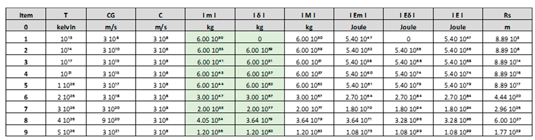m = 1.20 10⁵⁶ kg, total baryonic mass; δ = 1.20 10⁸² kg, total mass of dark matter.

It is very important to make it clear, the expansion of the universe is a function of frequency, each frequency has a certain expansion.

The calculations that we are going to carry out are referenced to the fundamental frequency.

In the spectrum of sound waves of the CMB, the fundamental frequency corresponds to the peak of greatest amplitude or first peak.

ω = 2.0 rad/s, fundamental angular frequency

f = 0.317 Hz, fundamental frequency

λ = 1.000.000 light years

λ = 9.46 10²¹ m

c1 = 3 10²¹ m/s

t1 = 1.22 10¹³ s

Calculation of the expansion of space-time to today:

Distance travelled 1:

where e1 is the distance travelled 1, c1 = 3 10²¹ m/s and t 1= 1.22 10¹³ s:

e1 = c1 x t1

e1 = 3 10²¹ m/s x t = 1.22 10¹³ s

e1 = 3.66 10³⁴ m

Distance travelled 2:

where e2 is the distance travelled 2, c2 = 3 10⁸ m/s and t 2= 4.35 10¹⁷ s:

e2 = c2 x t2

e2 = 3 10⁸ m/s x 4.35 10¹⁷ s

e2 = 1.30 10²⁶ m

Total distance travelled:

e = e1 + e2

e = 3.66 10³⁴ m + 1.30 10²⁶ m

We know that the bandwidth of the spectrum goes from 10⁻¹³ s to approximately 10¹³s.

If we consider the time 10⁻¹ s, close to the fundamental frequency, important for its contribution, we can increase the space e, a power of 10.

Figure 4 represents the sound spectrum of the CMB, the fundamental frequency is defined by the first peak or the peak with the highest amplitude.

Figure 4. CMB Power Spectrum.

Figure 4. CMB Power Spectrum.

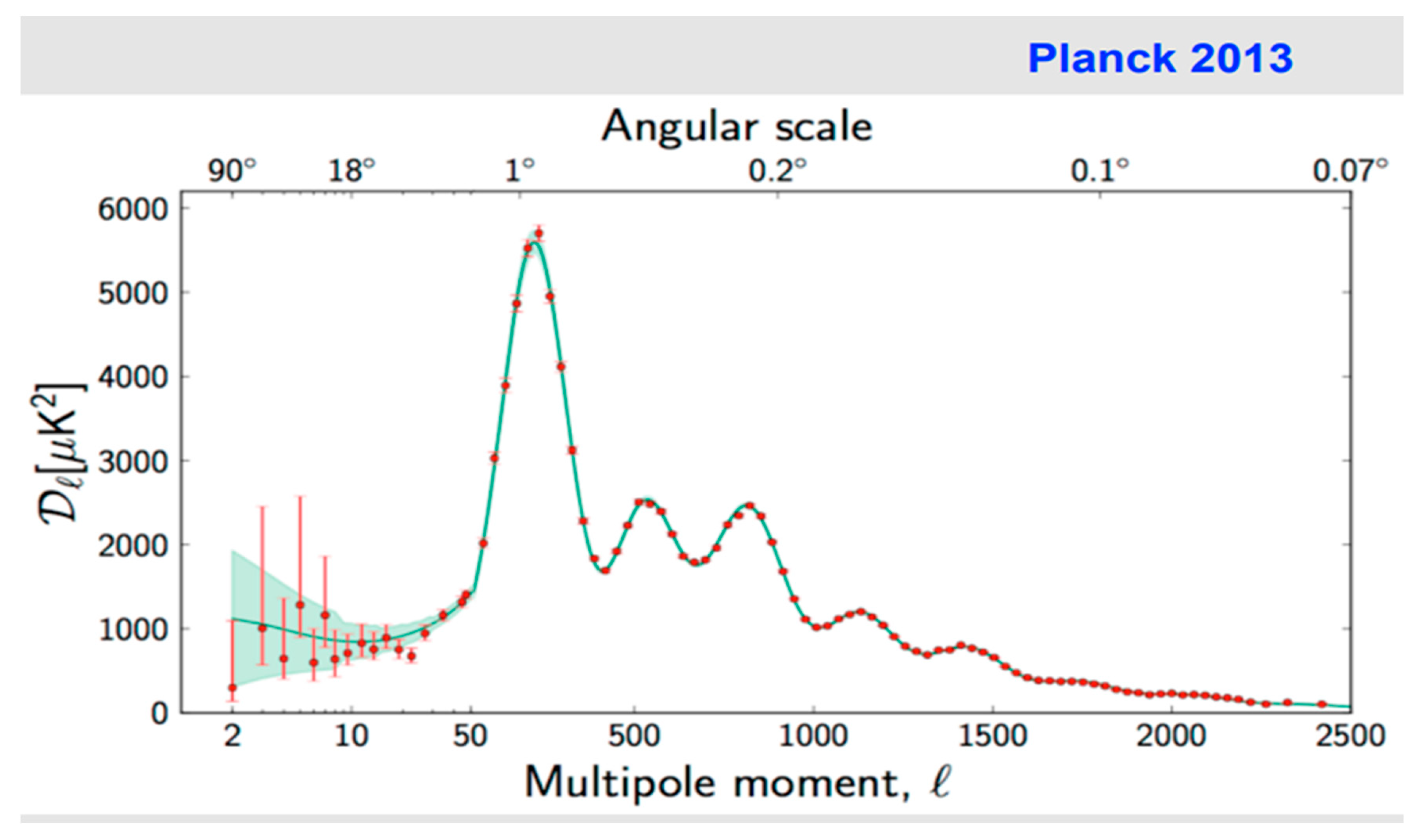
Although we have considered the contribution of the first peak to the right, we note that it is important to consider the contribution of the first peak to the left, that is why we consider the frequency content 10⁻¹ s before the fundamental frequency.

Therefore, the total distance covered will be:

e = 3.66 10³⁵ m

In one dimension, the universe will have the following radius:

Ru, radius of the universe:

Ru = 3.66 10³⁵ m

1 light-year = 9.46 10¹⁵ m

Ru = 3.66 10³⁵ / 9.46 10¹⁵

Ru = 3.86 10¹⁹ light-year

Knowing the radius of the universe, we will calculate the density.

Density equation:

ρ = m / v

Where ρ is density, m is mass, and v is volume.

v = 4/3 x π x R³

ρ = m / (4/3 x π x R³)

ρ = 1.20 10⁸² / (1.33 x 3.14 x 49.02 10¹⁰⁵)

ρ = 5.86 10⁻²⁶ kg/mᶾ

Density of the universe today.

ρo = 5.86 10⁻²⁹ g/cm³

Critical density of the universe today.

ρcr,o = 3.84 10⁻²⁹ g/cm3

Calculation of Ωᴍ,o:

Ωᴍ,o = ρo / ρcr,o

Ωᴍ,o = 5.86 10⁻²⁹ / 3.84 10⁻²⁹

According to the calculations:

Ωᴍ,o = 1.52; most probable value.

(I)

Another way to calculate Ωᴍ,o:

Ωᴍ,o = ρo / ρcr,o

ρo, density of the universe today

ρcr,o; critical density of the universe today

ρcr,o = 3.84 10⁻²⁹ g/cm³, UFSC data.

look at Figure 7

In item 9, the Schwarzschild’s radius corresponds to:

Rs = 1.77 10²⁹ m

We can call it the contraction factor of space-time or the compactification factor of matter.

Rc12 = 0.75 10⁻¹⁰ m, Radius of the atom carbon 12

Rq = 0.43 10⁻¹⁶ m, 100 times the radius of the quark.

Equation of volume of a sphere:

(4/3) π R³

Where R is the radius of the sphere.

Calculation of the volume of the atom carbon 12:

VaC12 = (4/3) x 3.14 x (0.75 10^-10⁻¹⁰) ³

VaC12 = 1.76 10⁻³⁰ m³, volume of C12 atom.

Calculate the volume of a 100-quark:

Rq = 0.43 10⁻¹⁶ m, 100 times the radius of the quark

Vq = (4/3) x 3.14 x (0.43 10⁻¹⁶) ³

Vq = 0.33 10⁻⁴⁸ m³

Calculation of the contraction factor Vac12 / Vq:

Vac12 / Vq = 1.76 10⁻³⁰ m³ / 0.33 10⁻⁴⁸ m³

Vac12 / Vq = 5.33 10¹⁸

In three dimensions the space-time contraction factor is 5.33 10¹⁸ times.

In one dimension the space-time contraction factor is 1.74 10⁶ times.

Fc = 1.74 10⁶

The approximate expansion of space-time will be equal to the Schwarzschild radius multiplied the contraction factor of space-time in one dimension.

In one dimension, the universe will have the following radius:

Ru, radius of the universe:

Ru = Rs x Fc

Rs, Schwarzschild radius.

Fc, contraction factor of space-time in one dimension.

Ru = 1.77 10²⁹ m x 1.74 10⁶ m

Ru = 3.09 10³⁵ m

Knowing the radius of the universe, we will calculate the density.

Density equation:

ρ = m / v

Where ρ is density, m is mass, and v is volume.

v = 4/3 x π x R³

ρ = m / (4/3 x π x R³)

ρ = 0.00971 10⁻²³

ρ = 9.71 10⁻²⁶ kg/m³

ρ = 9.71 10⁻²⁹ g/cm³

Density of the universe today.

ρo = 9.71 10⁻²⁹ g/cm³

Critical density of the universe today.

ρcr,o = 3.84 10⁻²⁹ g/cm³

Calculation of Ωᴍ,o:

Ωᴍ,o = ρo / ρcr,o

Ωᴍ,o = 9.71 10⁻²⁹ g/cm3/ 3.84 10⁻²⁹ g/cm³

According to the calculations:

Ωᴍ,o = 2.52

Calculate Ωᴍ,∞; for t → ∞:

(III)

Ωᴍ,∞ = ρ∞ / ρcr,o

ρ,∞; density of the universe for t → ∞

ρcr,o; critical density of the universe today

ρcr,o = 3.84 10⁻²⁹ g/cm³, UFSC data.

look at Figure 7

In item 9, the Schwarzschild’s radius corresponds to:

Rs = 1.77 10²⁹ m

We can call it the contraction factor of space-time or the compactification factor of matter.

Boltzmann’s constant for flat space-time, is defined for 1 mole of carbon 12 and corresponds to 6.0221 10²³ atoms.

We assume the ratio of the quark given by the German accelerator HERA (Hadron-Elektron-Ringanlage) in the year of 2016, whose article is published following the right of the internet (21).

Rc12 = 0.75 10⁻¹⁰ m, Radius of the atom carbon 12

Rq = 0.43 10⁻¹⁸ m, radius of the quark

Equation of volume of a sphere:

(4/3) π R³

Where R is the radius of the sphere.

Calculation of the volume of the atom carbon 12:

VaC12 = (4/3) x 3.14 x (0.75 10^-10⁻¹⁰) ³

VaC12 = 1.76 10⁻³⁰ m³, volume of C12 atom.

Calculate the volume of a quark:

Rq = 0.43 10⁻¹⁸ m, radius of the quark

Vq = (4/3) x 3.14 x (0.43 10⁻¹⁸) ³

Vq = 0.33 10⁻⁵⁴ m³

Calculation of the contraction factor Vac12 / Vq:

Vac12 / Vq = 1.76 10⁻³⁰ m³ / 0.33 10⁻⁵⁴ m³

Vac12 / Vq = 5.33 10²⁴

In three dimensions the space-time contraction factor is 5.33 10²⁴ times.

In one dimension the space-time contraction factor is 1.74 10⁸ times.

Fc = 1.74 10⁸

The approximate expansion of space-time will be equal to the Schwarzschild radius multiplied the contraction factor of space-time in one dimension.

In one dimension, the universe will have the following radius:

Ru, radius of the universe:

Ru = Rs x Fc

Rs, Schwarzschild radius.

Fc, contraction factor of space-time in one dimension.

Ru = 1.77 10²⁹ m x 1.74 10⁸ m

Ru = 3.07 10³⁷ m

Knowing the radius of the universe, we will calculate the density.

Density equation:

ρ = m / v

Where ρ is density, m is mass, and v is volume.

v = 4/3 x π x R³

ρ,∞= m / (4/3 x π x R³)

ρ,∞ = 0.00971 10⁻²⁹

ρ,∞ = 9.71 10⁻³² kg/m³

ρ,∞ = 9.71 10⁻³⁵ g/cm³

Density of the universe for t → ∞.

ρ,∞ = 9.71 10⁻³⁵ g/cm³

Critical density of the universe today.

ρcr,o = 3.84 10⁻²⁹ g/cm3

Calculation of Ωᴍ,∞:

Ωᴍ,∞ = ρ,∞ / ρcr,o

Ωᴍ,∞ = 9.71 10⁻³⁵ g/cm3/ 3.84 10⁻²⁹ g/cm3

According to the calculations:

Ωᴍ,∞ = 2.52 10⁻⁶ for t → ∞

6.7. We will demonstrate how the expansion of space-time as a function of frequency is asymmetry, that is, a variation in time gives us a variation in displacement.

In the damped RLC model, the fundamental frequency is the resonant frequency.

λ = λ0 = 1,000,000 light years

λ = λ0 = 9.46 10²¹m

ω = ω0 = 2 rad /s.

f0 = 0.31 Hz

low cut-off frequency calculation

ω1 = 1.81 10⁻¹¹ rad/s

f1 = 2.88 10⁻¹¹ Hz; low cut-off frequency

λ1 = 1.08 10³³ m

High cut-off frequency calculation:

ω2 = 2.19 10¹¹ rad/s

f2 = 0.348 10¹¹ Hz; high cut-off frequency

λ2 = 8.60 10¹⁰ m

For the low cut-off frequency, it is fulfilled:

$$E\left(\omega 1\right)=0.707Emax$$

(41)

$$\mathrm{E}\left(\mathrm{t}\right)=1.08 {10}^{73}\{{\mathrm{e}}^{^}-(1.81 {10}^{-11\mathrm{t}}\left)\right\}–1.08 {10}^{73}\{{\mathrm{e}}^{^}-(2.19 {10}^{11\mathrm{t}}\left)\right\}+\mathrm{E}\mathrm{o}$$

(42)

If we replace (41) in (42)

0.707 = 1 / e ⁻ (1.81 10⁻¹¹ᵗ)

t = ln (1.41) / 1.81 10⁻¹¹

t = 0.3467 / 1.81 10⁻¹¹

t1 = 1.915 10¹⁰ s

For the high cut-off frequency, it is fulfilled:

$$E\left(\omega 2\right) = 0.707 Emax$$

(43)

If we replace (43) in (42)

0.707 = 1 / e - (2.19 10¹¹ᵗ)

t = ln (1.41) / 2.19 10¹¹

t = 0.3467 / 2.19 10¹¹

t2 = 0.158 ⁻¹¹ s

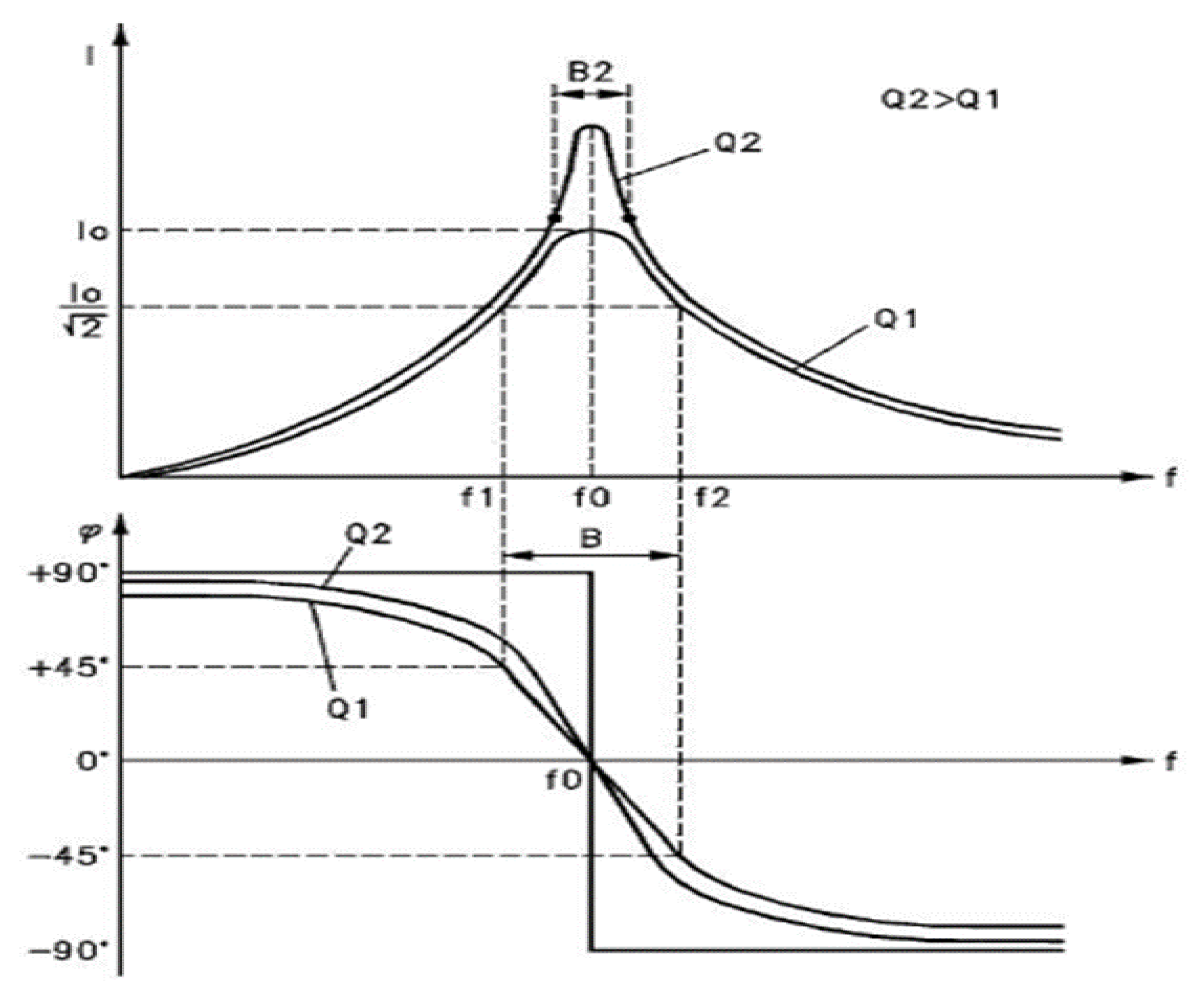
Observe Figure 5, we are going to calculate the time variation IΔtI between the frequency ω2 and ω1.

IΔtI = I t2 – t1I

IΔtI = I 0.158 ⁻¹¹ s - (- 1.915 10¹⁰ s) I

Consider that t1 originates much earlier than t2

IΔtI = 1.915 10¹⁰ s

This variation of time occurs within the interval of expansion of space-time, inside the bandwidth of the equation of gravitational waves, therefore its speed corresponds to 3 10²¹ m/s.

We will calculate the displacement variation IΔXI for a variation of IΔtI = 1.915 10¹⁰ s.

IΔXI = v x t

IΔXI = 3 10²¹ x 1.915 10¹⁰

IΔXI = 5.745 10³¹ m.

For the instant at which ω2 occurs, ω1 advances ω2 by 90 degrees and this corresponds to a time difference IΔtI = 1.915 10¹⁰ s, and a difference in displacement IΔXI = 5.745 10³¹ m.

We show how space-time, as a function of frequency, expands asymmetrically.

Figure 5. For a frequency difference given by ω2 and ω1, we can observe that there is a phase difference, a time difference and therefore a displacement difference IΔtI.

Figure 5. For a frequency difference given by ω2 and ω1, we can observe that there is a phase difference, a time difference and therefore a displacement difference IΔtI.

7. Conclusions:

Through the calculations and analysis carried out in item 6), it is possible to demonstrate that the theory proposed in items 1) to 5), is a theory that complements the Lambda-CDM model, in which several of the important calculations that predict the theory of the RLC electric model of the universe conforms to the predictions of the Lambda CDM model.

It was also possible to demonstrate, how the curvature of space-time is measured, by means of the theory of the generalization of space-time for curved space-time, fundamental, for the theory of the RLC electrical model of the universe to work.

The RLC electric model theory of the universe generalizes the Lambda-CDM model theory and predicts the origin of the universe, the origin of cosmic inflation, the origin of dark matter and the origin of dark energy. It also solves the horizon problem and demonstrates how the universe is flat and uniform.

References

- Gival Pordeus da Silva Neto. Estimando parâmetros cosmológicos a partir de dados observacionais. Departamento de Física Teórica e Experimental, Universidade Federal do Rio Grande do Norte. file:///C:/Users/Hecto/Downloads/Estimando_parametros_cosmologicos_a_partir_de_dado.pdf.
- Aurelio Carnero Rosell, Director Eusebio Sánchez Álvaro, Madrid, 2011. Determinación de parámetros cosmológicos usando oscilaciones acústicas de bariones en cartografiados fotométricos de galáxias. TESIS DOCTORAL, UNIVERSIDAD COMPLUTENSE DE MADRID. https://eprints.ucm.es/13761/1/T33317.pdf.
- Anderson Luiz Brandão de Souza, Orientador: Pedro Cunha de Holanda. Oscilações Acústica Bariõnicas. TESIS DE MESTRADO, Universidade Estadual de Campinas, Instituto de Física “Gleb. Wataghin”, Campinas 2018. https://sites.ifi.unicamp.br/sobreira/files/2018/07/mestrado-tanderson.pdf.
- JEFF STEIHAUER. Observation of quantum Hawking radiation and its entanglement in an analogue black hole. https://arxiv.org/abs/1510.00621.
- JEFF STEIHAUER. Spontaneous Hawking radiation and beyond: Observing the time evolution of an analogue black hole. https://arxiv.org/abs/1910.09363.
- Quando a Luz se curvou. https://revistapesquisa.fapesp.br/quando-a-luz-se-curvou/.
- J.S.Farnes. A Unifying Theory of Dark Energy and Dark Matter: Negative Masses and Matter Creation within a Modified ΛCDM Framework. https://arxiv.org/abs/1712.07962.
- Alberto Casas, Profesor de Investigación IFT, CSIC/UAM. La luz y el origen de la materia. https://www.youtube.com/watch?v=CTrX_JBNEnU.
- Eisberg Resnick, Física Cuántica.
- Eyvind, H. Wichmann. Física cuántica.
- Sears – Zemansky. Física Universitaria con Física Moderna Vol II.
- Iván García Brao. Ecuación de campo de Einstein, Universidad de Murcia, Facultad de Matemáticas. Trabajo de grado año 2018. https://www.um.es/documents/118351/9850492/Garc%C3%ADa+Brao+TF_77837970.pdf/debaa03b-605b-420d-b3ac-85549b6622c0.
- Luis Felipe de Oliveira Guimarães, Orientadora Maria Emilia Xavier Guimarães. Soluciones de buracos negros na relatividade general, Universidad federal Fluminense, Bacherelado em Física. Trabajo de grado 2015. https://app.uff.br/riuff/bitstream/handle/1/5977/Luiz%20Filipe%20Guimaraes.pdf;jsessionid=4EAAF6CB7A4B776D04C9E6E6573D5919?sequence=1.
- Kostas kokkotas, Field Theory.
- James, B. Hartle, Gravity and introduction to Einstein’s General Relativity.
- Charles, W. Misner, Kip S. Thorne and Jhon Archibald Wheelher, Gravitation.
- Benito Marcote, Cosmologia Cuantica y creacion del universe.
- Carlos Rovelli, Quantum Gravity.
- Vinicius Miranda Bragança, Singularidades em teorias f(r) da gravitação. http://arcos.if.ufrj.br/teses/mestrado_vinicius_miranda.pdf.
- Laurent Pitre ∗, Mark D. Plimmer, Fernando Sparasci, Marc E. Himbert; 2019. Determinations of the Boltzmann constant. https://hal.science/hal-02166573/file/1-s2.0-S1631070518301348-main.pdf.
- ZEUS Collaboration, 2016. Limits on the effective quark radius from inclusive ep scattering at HERA. Accepted for publication in Physics Letters B. https://arxiv.org/pdf/1604.01280.pdf.
Disclaimer/Publisher’s Note: The statements, opinions and data contained in all publications are solely those of the individual author(s) and contributor(s) and not of MDPI and/or the editor(s). MDPI and/or the editor(s) disclaim responsibility for any injury to people or property resulting from any ideas, methods, instructions or products referred to in the content. |
© 2023 by the authors. Licensee MDPI, Basel, Switzerland. This article is an open access article distributed under the terms and conditions of the Creative Commons Attribution (CC BY) license (http://creativecommons.org/licenses/by/4.0/).
Copyright: This open access article is published under a Creative Commons CC BY 4.0 license, which permit the free download, distribution, and reuse, provided that the author and preprint are cited in any reuse.