
Submitted:
28 April 2023
Posted:
05 May 2023
You are already at the latest version
Abstract
Winter frost injury is a major limiting factor for olive cultivation in temperate regions. The response of olive shoots to freezing stress can be used for selecting resistant genotypes to freezing. The electrolyte leakage (EL) and tetrazolium tests (TZ) are commonly used to evaluate dead tissues in cold stress studies. The temperature-response curve of dead tissues to lethal temperature (LT) is measured with models to calculate LT50 and LT90. In this study, we evaluated the accuracy and efficiency of eighteen non-linear regression models (NLRs) in calculating LT50 and LT90 of freezing stress in different olive cultivars at various stages of dormancy. After evaluating the prediction performance of NLR models, it was found that only eight models were suitable for the purpose of this research out of the 18 models examined. The 2p-logistic and Gompertz models were selected for modeling EL and TZ, respectively. Our research findings indicate that the Roughani, Kawi, and Zard varieties of olive trees exhibit the best performance in cold weather conditions. Our findings provide valuable insights into selecting frost-resistant cultivars and designing effective strategies for cold acclimation in olive cultivation.
Keywords:
olive trees
; freezing injury
; electrolyte leakage
; tetrazolium tests
; nonlinear regression models
1. Introduction
Olive trees are a subtropical crop that can thrive in certain temperate regions as well. The Mediterranean Basin heavily relies on the economic benefits of olive oil, which is extracted from the fruit of the olive tree. In addition to serving as a vital economic resource, table olives are also a popular food item [[1]]. However, due to their subtropical nature, olive trees are highly vulnerable to winter frost injury [[2]]. Numerous studies have been conducted to select frost-resistant cultivars of olive trees [[3]]. Some studies typically involve evaluating different cultivars based on their performance during natural frost events [[4]]. Most studies have also evaluated the viability of shoot tissue from different genotypes under controlled freezing temperatures [[5,6]]. The electrolyte leakage and tetrazolium tests are two important indicators used in the screening of plant frost injury, particularly in cold stress studies, to assess the presence of dead tissue. Electrolyte leakage (EL) is determined by measuring the ratio of ion leakage from injured tissues to intact tissues using electrical conductivity. Meanwhile, dead tissues are identified via staining and visually scored in the tetrazolium test (TZ). To screen for frost-hardy resistant genotypes, plant tissues at various stages of growth are exposed to controlled freezing temperatures. By determining the temperature at which 50% of tissues are lost (known as the lethal temperature or LT50) with computing models can designate the degree of genotype resistance to freezing stresses. The typical response of plant tissues to a series of freezing temperatures is an asymmetric sigmoid curve [[7]]. Probit analysis has been a commonly used method to determine LT50 in many studies related to freezing stress in plants, including olive trees [[2]]. Regression models such as linear interpolation, Richards, logistic, and Gompertz models have also been used for LT50 estimation in some studies [[5,7-9]]. Nonlinear regression is a statistical method used to model the relationship between a dependent variable and one or more independent variables when the relationship is not linear. In the context of freezing injury, nonlinear regression can be used to model the relationship between the extent of tissue damage and the temperature and duration of exposure to freezing temperatures [[8,9]]. This type of analysis can help researchers understand the factors that contribute to freezing injury and develop strategies to mitigate its effects. Nonlinear regression models can be more complex than linear regression models, and may require more sophisticated statistical techniques to fit to the data [[10]]. However, they can often provide a better fit to the data and more accurate predictions than linear models when the relationship between the variables is not linear [[10]]. Overall, nonlinear regression can be a powerful tool for analyzing the complex relationships between freezing injury and duration of exposure and can help researchers develop a better understanding of this phenomenon.
During the growing season, the optimal temperature range for olive trees is around 20-30°C. While olive trees can withstand minimum temperatures of about -4°C in winter and maximum temperatures of about 50°C in hot and dry summers, sub-optimal and chilling temperatures (between 7.5 and 12.5°C) can significantly slow down metabolic processes such as respiration and photosynthesis. Freezing temperatures, defined as temperatures averaging below -10°C, can cause irreparable damage to organs and tissues, and in severe cases, the entire plant can die [[2]]. Freezing stress is often more damaging to olive trees than chilling stress. The temperature threshold for frost damage in olive trees varies depending on factors such as genotype, growth conditions, and the timing of the low temperatures (early frost, winter frost, or late frost). Additionally, the hardening or de-hardening phase of the tree can also impact its susceptibility to frost damage [[11-14]]. [Larcher [15]] reported that the LT50 of olive twig cambium and xylem was -16°C. [Bartolozzi and Fontanazza [16]] showed that the LT50 of higher resistance olive cultivars, such as 'Bouteillan' and 'Nostrale di Rigali', were -18.2 and -18.1°C, respectively, while the LT50 of lower tolerance of 'Borsciona' and 'Morcona' were -12.28 and -11.48°C, respectively. In addition to the effects of genotype, the severity of damage caused by freezing stress in olive trees can depend on a range of factors, including the duration of the freezing event, the stage of plant growth, and the cold acclimation or dormancy processes [[17]]. A series of physiological and metabolic changes occur during the cold acclimation process, which prepares olive trees for low-temperature tolerance. [Cansev, et al. [18]] evaluated the cold hardiness of twelve olive cultivars and found that cold acclimation increased the freezing tolerance of these cultivars. Osmolytes, such as soluble carbohydrates and proline, play a crucial role in the resistance of woody plants to freezing stress [[2]]. By accumulating these compounds, plants can protect themselves from the damage caused by ice formation [[17]].
The majority of published articles in the domain of fruit freezing process modeling have utilized a limited number of non-linear regression models, with many employing various models. Consequently, this article presents a comprehensive review of non-linear regression models for the olive fruit within this field. The objectives of the paper are outlined as follows: (1) evaluate the fitness of 18 computing models in pre-, deep, and post dormancy of ten olive cultivars under freezing temperature, and (2) Accuracy and sensitivity analysis were compared in each model (3) Prediction of plant response with selected models at out-of-range temperatures.
2. Materials and Methods:
2.1. Olive Cultivars and Orchard Management:
Ten olive cultivars 'Dorsalani', 'Luke', 'Roughani', 'Shangeh', 'Rashid', 'Mission', 'Kawi', 'Abu-Stal', 'Manzanilla', and 'Zard' (coded as CV1 to CV10) were sampled at three different times - before, during, and after dormancy, corresponding to November, January, and March. The olive trees were grown in an adaptation collection established in 2001, using a randomized complete block design (RCBD) with four replications and six trees in each plot. The trees were spaced 4x6 meters apart and were 20 years old at the time of sampling. The orchard management included regular irrigation and fertilization, and the trees were free of pests and nutritional deficiencies.
2.2. Temperature Treatments
One-year-old shoots, 30 cm long and 1 cm in diameter, were collected from each olive cultivar in the germplasm collection and immediately transported to the laboratory. After removing the leaves and washing the branches with distilled water, the shoots were cut into smaller pieces, 1 cm in length, at the internodal distances. The pieces were then placed in a cold room at 4°C for 3 hours. Subsequently, the samples were subjected to a stepwise freezing process from 0 to -21°C (0, -3, -6, -9, -12, -15, -18, and -21°C) using a freezing test device (Kimiya Rahvard Co. Iran). The freezing rate was set at 3°C hour-1, and the duration of each test temperature was 60 minutes. At each stage, after cold treatment at the desired temperature, the samples were removed from the freezing test device and used for electrolyte leakage and tetrazolium tests.
2.3. Electrolyte leakage (EL)
To evaluate the extent of freezing damage on cell membranes, the rate of electrolyte leakage (EL) was calculated following the method of Equation (1). Stem samples from each temperature treatment (ranging from 0 to -21°C) were placed in 40 ml of distilled water at room temperature for 24 hours. The electrical conductivity (EC1) was measured using an EC meter (Con500, Korea). The samples were then autoclaved at 120°C for 2 hours, and after cooling to room temperature, their ion leakage was measured using an EC meter (EC2). The percentage of conductivity was calculated for each sample using the ratio of the initial to the final measurements multiplied by 100.
2.4. Triphenyl tetrazolium chloride (TZ) assay
The tetrazolium staining method was used to determine the percentage of dead tissues. Stem samples from each temperature treatment were placed in a test tube containing 5 ml of 1% 5-3-2-triphenyltetrazolium chloride solution and kept in the dark at room temperature for 24 hours. The samples were then cut into thin sections using a microtome machine and observed under a light microscope. The extent of visual damage was measured as a percentage based on the staining of dead tissues in the phloem and cambium layers at the outer circle of the shoot pieces.
2.5. Nonlinear regression models (NLRs)
Eighteen nonlinear regression models (NLRs) were used to fitting to freezing injury on olive cultivars (Table 1). Other research efforts have included only one or two models [[5,8,12]]. One important aspect of developing a NLR model for freezing injury is choosing the appropriate functional form for the model. NLR models can take on a variety of forms, including polynomial, exponential, logarithmic, and sigmoidal functions, among others. The choice of functional form will depend on the nature of the relationship between the independent and dependent variables, as well as the specific research question being addressed and based on prior knowledge or theory about the relationship between the dependent and independent variables.
The relationship between dependent variables (EL and TZ) and independent variable (temperature) was analyzed using non-linear regression. NLR models were fit using the fitnlm function in MATLAB software using the Levenberg-Marquardt (LM) algorithm that minimized the sum of squares error (SSE) between the predicted and observed values of EL and TZ. NLR models are often fit using iterative algorithm such as the LM. This algorithm iteratively adjust the parameters of the NLR until a minimum in the SSE is reached. NLR algorithms can be sensitive to the initial parameter values, and different initial values can lead to different solutions. One common method for addressing this is to use multiple initial values and choose the best solution based on some criterion, such as the SSE. We used the cftool graphical interface in MATLAB to explore the data and select an appropriate starting point for the parameter estimates. The model was fit separately to the EL and TZ data, using the temperature data as the predictor variable and the EL and TZ as the response variables. Statistical significance was set at p < 0.05. To assess the goodness of fit of the NLR model, we calculated the coefficient of determination (R2), adjusted coefficient of determination (), residuals, normal probability plots of residuals, and the root mean squared error (RMSE). Before conducting the NLR analysis, the data were preprocessed to remove any outliers or missing values. The data were also checked for normality using the Shapiro-Wilk test, and transformed if necessary to meet the assumptions of the NLR model.
3. Results and discussion
In this section of the article, we present the results under two headings: the modeling results of EL and TZ. We examine the non-linear regression models for each indicator separately and calculate the T50 and T90 values using the best-fitted model. Finally, we evaluate the cold tolerance of different olive varieties based on their resistance to freezing injury and provide recommendations for further discussion.
3.1. Findings of the electrolyte leakage (EL) assay
3.1.1. Comparing and selecting the best-fitted NLR model for EL
As stated in the preceding section, eighteen models were employed to estimate the EL of ten distinct olive cultivars. The fitting outcomes of these models revealed that only eight of them exhibited a superior ability to predict EL, while the remaining models did not perform significantly worse in terms of prediction accuracy. Table 2 displays the RMSE values of eight models used to estimate EL in pre, deep, and post-dormancy of ten olive cultivars. The results reveal that the rank of the models differed in terms of RMSE, indicating that the choice of the appropriate model for each cultivar and its dormancy stage is crucial. M7, M9, M15, and M16 models performed poorly compared to the other models, while M2, M3, M4, M5, M6, M8, M10, and M14 were identified as the best options. However, some models, such as M8, had lower prediction errors, but their coefficients were not significant. Further analysis showed that some models overestimated EL by more than 100% across the tested temperature range, including lower temperatures. After considering the significance of coefficients, simplicity of application, and generalizability, the M3 model was selected for all varieties and assessment stages. This allows for comparing the varieties and their stages by comparing the coefficients' values of the NLR models. The lowest and highest RMSE values across all cases were 3.29% and 9.06%, respectively. These findings suggest that choosing the appropriate model is crucial for accurate estimation of EL, and the M3 model is a reliable option for all varieties and assessment stages.
3.1.2. Assessment of NLR model coefficients for EL
After choosing the 2p-logistic model (M3) as the selected model to predict EL in terms of temperature for different olive cultivars, its coefficient estimates were computed using the fitnlm function in MATLAB software. The ANOVA table and then the significance assessment of the model coefficients were also obtained using it. Table 3 displays the coefficient values, standard deviation, and significance results for the nonlinear regression model (M3) used to predict EL across ten different olive cultivars during three dormancy stages. Additionally, the table presents the corresponding R2 and values. The results indicate that both model coefficients, b1 and b2, are significant at the 1% level for all cases. These findings demonstrate that the M3 model is appropriate and applicable for all cases, with R2 and values ranging from 83% to 96%. Thus, the selected regression model has successfully explained approximately 83% to 96% of the observed EL changes based on the experimental results.
3.1.3. Conducting a sensitivity analysis of the EL model
To better understand the behavior of the M3 model, we plotted the EL predictions against temperatures below zero while varying the regression coefficients b1 and b2 (Figure 1). The graph shows that increasing the regression coefficient b2 results in a steeper slope of EL changes with respect to temperature. Consequently, olive cultivars with higher b2 values reach an EL value of 100% sooner, indicating greater sensitivity to cold temperatures. For instance, when b2 equals 0.05 and 0.20, the EL value reaches 100% at temperatures higher than -70 and about -30°C, respectively. On the other hand, an increase in the regression coefficient b1 leads to a shallower slope of EL changes with respect to temperature. However, changes in b1 do not affect the temperature required to achieve an EL value of 100%. Notably, lower values of b1 indicate greater sensitivity of the olive to cold temperatures, while the opposite may also be true.
3.1.4. Comparison of EL modeling outcomes for different olive cultivars
The Supporting Information section of the article includes the prediction results of the M3 model for the EL parameter of olive trees at tested temperatures, as well as the lower and upper bounds of the prediction for the three stages of pre, deep, and post-dormancy for ten olive cultivars. The results presented in Figure S1 demonstrate that the M3 model provided estimates of EL that fell within the 95% prediction interval of the model for most of the laboratory data. Although some observed values deviated slightly from the predicted values at certain temperatures, the overall results were deemed acceptable. Additionally, the coefficient of determination supported the accuracy of the model.
Figure 2 depicts the extrapolated results of EL modeling for each of the ten olive cultivars at the pre, deep, and post-dormancy stages, up to a temperature of -50 °C. The results of this study indicate that the pre, deep, and post-dormancy stages of olive trees during temperature reduction to -50°C are associated with high-to-low estimation of EL. The models of deep and post dormancy stages are very similar, while the pre-dormancy model differs significantly. These findings suggest that olive trees are particularly vulnerable to freezing injury during the pre-dormant stage. It is important for olive growerss to be aware of this vulnerability and take appropriate measures. If the pre-dormancy stage is successfully managed, olive trees can adapt to their environment and improve their resistance to freezing injury [[18]]. Comparing the tolerance of ten different olive cultivars to freezing injury in terms of EL at both the deep-dormancy and post-dormancy stages revealed that the cultivars CV10, CV7, CV1, CV4, CV2, CV8, CV5, CV9, CV3, and CV6 exhibited the highest-to-lowest resistance to freezing injury. The ranking of olive cultivars according to their resistance to freezing injury during the pre-dormancy stage was as follows: CV3, CV10, CV7, CV4, CV1, CV9, CV6, CV2, CV5, and CV8. These findings can help in selecting appropriate olive cultivars based on the prevailing climatic conditions and other management considerations in the region.
3.1.5. Analysis of the rate of change in EL results
The NLR model can be applied to calculate the rate of EL changes per decrease in sub-zero temperature. To achieve this, the first-order derivative is taken from the NLR regression function. Figure 3 shows the track of EL changes for ten olive cultivars in the pre, deep, and post-dormancy stages. The results demonstrate that at the beginning of exposure to cold and sub-zero temperatures, the increasing EL rate gradually decreases until a certain temperature, such as -15° C, after which it changes to an upward trend. In freezing stresses of plants, Ice crystal formation can occur intracellularly and extracellularly. Extracellular ice formation occurs at an early stage when the temperature drops below the freezing point. Due to the latent heat of water, a slight increase or stabilization of temperature can be observed. However, as the temperature continues to drop or rapid freezing occurs, intracellular ice formation predominantly happens, leading to mechanical disruption of the protoplasmic structure and eventual cell death [[17]]. Furthermore, different olive cultivars exhibit varying reactions, with different starting temperatures for EL increase. In the Pre-dormancy stage, the starting temperature is smaller in absolute value than in the other two stages. Moreover, the rate of EL changes reaches a constant value sooner in the Pre-dormancy stage. This may be attributed to the lower concentration of osmolytes in the intercellular sap during the early stages of acclimation in olive trees [[18]]. The primary mechanism used by the tree to withstand winter cold is the accumulation of carbohydrates and osmolytes within its tissues [[17]]. However, in pre-dormancy stage, the concentration of these substances has not yet reached its maximum level, resulting in a narrower model curve during this stage. As so, the higher slope of the variation track indicates a greater sensitivity of the olive variety to freezing injury.
3.1.6. Assessment of T50 and T90 values based on the EL model in different olive varieties
Table 4 presents the calculated T50 and T90 temperatures for ten olive cultivars in three dormant stages, based on the NLR model. The T50 and T90 values provide important information about the cold tolerance of olive trees. These values indicate the temperatures at which a certain percentage of olive tree cells will be killed due to exposure to sub-zero temperatures. For example, in CV1 during the Pre-dormancy stage, the T50 and T90 values were obtained at temperatures of -5.26°C and -17.32°C, respectively. This means that at a temperature of -5.26°C, 50% of the maximum EL values were reached, and at a temperature of -17.32°C, 90% of the maximum EL values were reached. The lowest T50 value occurs in the pre-dormancy stage at -10.99°C in CV3, followed by CV10 at -10.58°C. The lowest T90 values across all stages (pre, deep, and post-dormancy) are observed in CV10 at -25.68°C, -43.53°C, and -38.28°C, respectively.
The T50 and T90 values for different olive cultivars have been widely studied as important indicators of cold tolerance. These values can provide insights into the potential of different cultivars for withstanding freezing injury, and can help in selecting more cold-tolerant cultivars for olive cultivation in regions with cold winters.
3.2. Findings of the triphenyl tetrazolium chloride (TZ) assay
3.2.1. Comparing and selecting the best-fitted NLR model for TZ
Apart from utilizing the EL measure of resistance against freezing injury, TZ was also employed. The prediction errors of all eighteen models mentioned in Table 1 were calculated for ten distinct olive cultivars across three stages of dormancy, i.e., pre, deep, and post-dormancy. However, only the results of the TZ for eight models are presented in Table 5. After evaluating the RMSE values of all models, it was observed that they were generally acceptable and close to each other, with only slight differences. However, a closer examination of their shapes at lower temperatures and the significance test of their regression coefficients revealed that models M3, M4, M5, M6, and M7 were the strongest candidates for selection. Ultimately, the M4 model was chosen as the final model to accurately model the process of TZ changes at sub-zero temperatures. This decision was based on its ability to better illustrate the nature of the TZ problem and investigate the phenomenon of freezing injury. Unlocking the secrets of complex systems demands a comprehensive approach. That's why we chose a single model type to analyze all three stages across various olive varieties. This approach grants us the power to scrutinize regression coefficients in a more accurate and relevant way, leading us to uncover a wealth of insights.
3.2.2. Assessment of NLR model coefficients for TZ
Table 6 presents the statistical analysis results for the coefficients of the Gompertz nonlinear regression model (M4), including the coefficients of determination (R2 and ) for all tested cases of olives. Our analysis of the M4 model revealed that the p-values of its coefficient significance test were significant at both the 1% and 5% levels across all olive varieties. This finding underscores the robustness of our model and the validity of our results. Our analysis of the coefficients of determination and the standard deviation of the regression coefficients revealed a remarkable consistency across all cases. By achieving R2 and values ranging from 92 to 98 percent, our study provides strong evidence for the robustness and precision of our approach.
3.2.3. Conducting a sensitivity analysis of the TZ model
The regression coefficients of the TZ model varied significantly among different olive cultivars, as presented in Table 6. Furthermore, the values of these coefficients also differed across the three stages of dormancy (i.e., pre, deep, and post-dormancy) within each olive cultivar. These differences can be attributed to variations in the response of different olive cultivars to freezing injury during each stage of dormancy. To gain a deeper understanding of this issue, we conducted a sensitivity analysis of the TZ model's predictions for sub-zero temperatures by examining the impact of changes in the b1 and b2 regression coefficients. As depicted in Figure 4 (a), an increase in the regression coefficient b2 corresponds to an increase in the slope of TZ changes during temperature decrease. Specifically, when b2 is set to 0.25, the maximum slope of changes is achieved, leading to an earlier and more pronounced decrease in TZ at lower temperatures. Conversely, when b2 is set to 0.1 (the lowest value obtained from the experiments), TZ reaches a value of approximately 100% at a temperature of about -55 °C. These findings suggest that b2 plays a crucial role in determining the rate and extent of TZ changes in response to sub-zero temperatures. Figure 4 (b) demonstrates that increasing the value of the regression coefficient b1 in the TZ model leads to a higher TZ value at the point of freezing. However, the effect of b1 on the temperature at which TZ reaches 100% is negligible, as this value is consistently attained at -37 °C across all b1 values. These findings suggest that a higher b1 value corresponds to greater resistance of olive trees to freezing injury, enabling them to better adapt to changing environmental conditions.
3.2.4. Comparison of TZ modeling outcomes across various olive cultivars
Initially, the models were evaluated based on laboratory results, and the best-performing model, M4, was selected. The Supporting Information section and Figure S2 present the lower and upper bounds, as well as the trend of changes predicted by the M4 model, alongside data from ten olive cultivars in pre, deep, and post-dormancy stages. The results indicate that the M4 model estimates and laboratory data fall within the 95% prediction interval. Table 6 additionally confirms the validity of the model estimates within the tested temperature range. Notably, the M4 model is capable of predicting TZ for temperatures beyond the test range, as demonstrated in Figure 5, where TZ values were extrapolated for ten olive cultivars across three dormancy stages, extending to temperatures as low as -50 °C. This extrapolation allows for predictions regarding tree behavior outside the testing period, with the model's horizontal asymptotic line reaching the 100% point across various temperatures. The results depicted in Figure 5 demonstrate that, for all three dormancy stages, the trends of changes and values of TZ predictions are largely similar across all olive cultivars. However, there is a slight variation in the predicted values of TZ for pre, deep, and post-dormancy stages, which create the highest to lowest values during temperature reduction. This may be attributed to the inherent nature of the olive tree, which exhibits resistance and adaptation to new conditions, including exposure to sub-zero temperatures [[13]].
In contrast to EL, which did not reach 100% even at temperatures below -50°C (as shown in Figure 2), the value of TZ reaches 100% in the temperature range of -25 to -35°C. Therefore, it can be inferred that the TZ criterion is more stringent in its judgments than the EL criterion. However, based on the EL criteria, its value varies in the range of 85 to 95 percent in the temperature range of -25 to -35 (as depicted in Figure 2).
Our findings indicate that olive cultivars with a higher amount of TZ during temperature drops in sub-zero conditions, and those that reach 100% TZ sooner, exhibit lower resistance to freezing injury. Based on these results, as well as the data presented in Figure 5 for the pre-dormancy stage, we can conclude that the olive tree cultivars CV6, CV5, CV9, CV8, CV2, CV4, CV1, CV7, CV3, and CV10 display a range of resistance and compatibility in sub-zero temperature conditions, with CV10 exhibiting the highest level of resistance and CV6 showing the lowest. In the Deep-dormancy stage, the olive cultivars can be ranked based on their adaptation or resistance to freezing injury, from the lowest to the highest, as follows: CV6, CV9, CV5, CV2, CV8, CV4, CV1, CV7, CV3, and CV10. After the dormancy period, we observed varying degrees of resistance to freezing injury among the olive cultivars. Based on our results, we sorted them in the following order: CV9, CV6, CV2, CV5, CV4, CV8, CV1, CV10, CV7, and CV3. Furthermore, our TZ modeling analysis revealed that CV6, CV9, and CV5 are the most compatible varieties in sub-zero temperature conditions. On the other hand, CV3, CV7, and CV10 showed the least compatibility with these conditions. Therefore, we suggest that CV6, CV9, and CV5 are the most suitable options for cultivation in areas with sub-zero temperatures, while CV3, CV7, and CV10 should be avoided.
3.2.5. Analysis of the rate of change in TZ results
As previously mentioned, we utilized the first-order derivative of the TZ regression model to determine the rate of change of TZ production with respect to temperature. Figure 3 illustrates the TZ production track for ten olive cultivars across three dormancy stages: pre, deep, and post-dormancy. Interestingly, we observed that the temperature point at which the TZ production rate changes is nearly constant across all three dormancy stages for each olive cultivar, in contrast to the EL results (Figure 3). The temperature range at which this phenomenon occurs varies from -5°C to -12°C. Additionally, our results indicate that the rate of TZ production reaches its minimum value and eventually reaches zero after the temperature drops below -35°C. Furthermore, we found that the slope of the TZ production decrease and increase is nearly identical. Comparing the three dormancy stages within each variety, we noted that the temperature at which the TZ production rate changes occurs earlier during the pre-dormancy stage compared to the other two stages. This suggests that olive trees lose their resistance to frost damage earlier during the pre-dormancy stage according to TZ analysis.
3.2.6. Assessment of T50 and T90 values based on the TZ model in different olive cultivars
Table 7 presents the T50 and T90 values calculated using the TZ model for ten different olive tree varieties across three dormant stages. T50 and T90 represent the temperature below which the TZ value is equal to 50% and 90%, respectively. Higher absolute values of T50 and T90 indicate greater resistance to freezing injury and better adaptability to sub-zero temperatures. CV10, CV3, and CV7 demonstrated the highest performance across all three dormancy stages based on T50 values. Moreover, these three cultivars were also the best options across all three dormant stages based on T90 values. Hence, in terms of TZ criteria, these three selections could be considered as suitable breeding options for temperate zone compared to the other seven varieties.
4. Conclusion
This study evaluated the resistance and compatibility of ten olive cultivars to sub-zero temperatures and frost damage during three stages of dormancy using electrolyte leakage (EL) and tetrazolium tests (TZ) with the help of NLR analysis utilizing 18 different models. Eight models were selected based on significant regression coefficients, extrapolation results, trend of changes in model prediction, and R2 and criteria. The 2p-logistic model and Gompertz model were selected for EL and TZ criteria, respectively. The NLR model allowed for the identification of the relationship between temperature and olive tree freezing injury, and the development of a predictive model for estimating the extent of tree damage and time to zero growth based on temperature data. The study identified the three cultivars CV10, CV7, and CV3 as having the best performance in sub-zero temperature conditions, with better resistance and adaptability to frost damage. However, it is important to note that the NLR model developed in this study is specific to the observed study conditions and may not be applicable to other locations or climates. Additionally, other factors such as wind speed, humidity, and soil moisture may also influence freezing injury in olive trees, which were not examined in this analysis. Overall, this research provides valuable information for olive growers and researchers to develop strategies to manage cold weather effects and prevent freezing injury in olive orchards.
Conflicts of Interest
The authors declare no conflict of interest.
References
- Dahdouh, A.; Khay, I.; Le Brech, Y.; El Maakoul, A.; Bakhouya, M. Olive oil industry: a review of waste stream composition, environmental impacts, and energy valorization paths. Environ. Sci. Pollut. Res. 2023, 30, 45473–45497. [Google Scholar] [CrossRef] [PubMed]
- Petruccelli, R.; Bartolini, G.; Ganino, T.; Zelasco, S.; Lombardo, L.; Perri, E.; Durante, M.; Bernardi, R. Cold Stress, Freezing Adaptation, Varietal Susceptibility of Olea europaea L.: A Review. Plants 2022, 11, 1367. [Google Scholar] [CrossRef] [PubMed]
- Bartolozzi, F.; Fontanazza, G. Assessment of frost tolerance in olive (Olea europaea L.). Sci. Hortic. 1999, 81, 309–319. [Google Scholar] [CrossRef]
- Cansev, A.; Gulen, H.; Eris, A. Cold-hardiness of olive (Olea europaeaL.) cultivars in cold-acclimated and non-acclimated stages: seasonal alteration of antioxidative enzymes and dehydrin-like proteins. J. Agric. Sci. 2008, 147, 51–61. [Google Scholar] [CrossRef]
- Lodolini, E.; Alfei, B.; Santinelli, A.; Cioccolanti, T.; Polverigiani, S.; Neri, D. Frost tolerance of 24 olive cultivars and subsequent vegetative re-sprouting as indication of recovery ability. Sci. Hortic. 2016, 211, 152–157. [Google Scholar] [CrossRef]
- López-Bernal, .; García-Tejera, O.; Testi, L.; Orgaz, F.; Villalobos, F.J. Studying and modelling winter dormancy in olive trees. Agric. For. Meteorol. 2019, 280, 107776. [CrossRef]
- Yuldasheva, K.T.; Soliyeva, M.; Kimsanova, X.; Arabboev, A.; Kayumova, S. Evaluation of winter frost resistance of cultivated varieties of olives. Acad. Int. Multidiscip. Res. J. 2021, 11, 627–632. [Google Scholar] [CrossRef]
- Gómez-Del-Campo, M.; Barranco, D. Field evaluation of frost tolerance in 10 olive cultivars. Plant Genet. Resour. Charact. Util. 2005, 3, 385–390. [Google Scholar] [CrossRef]
- Lindén, L.; Palonen, P.; Lindén, M. Relating Freeze-induced Electrolyte Leakage Measurements to Lethal Temperature in Red Raspberry. J. Am. Soc. Hortic. Sci. 2000, 125, 429–435. [Google Scholar] [CrossRef]
- Murray, M.B.; Cape, J.N.; Fowler, D. Quantification of frost damage in plant tissues by rates of electrolyte leakage. New Phytol. 1989, 113, 307–311. [Google Scholar] [CrossRef]
- Lim, C.C.; Arora, R.; Townsend, E.C. Comparing Gompertz and Richards Functions to Estimate Freezing Injury in Rhododendron Using Electrolyte Leakage. J. Am. Soc. Hortic. Sci. 1998, 123, 246–252. [Google Scholar] [CrossRef]
- Tudela, V.; Santibáñez, F. Modelling impact of freezing temperatures on reproductive organs of deciduous fruit trees. Agric. For. Meteorol. 2016, 226-227, 28–36. [Google Scholar] [CrossRef]
- Villouta, C.; Workmaster, B. A.; Atucha, A. , Freezing stress damage and growth viability in Vaccinium macrocarpon Ait. bud structures. Physiologia Plantarum 2021, 172(4), 2238–2250. [Google Scholar] [CrossRef] [PubMed]
- Archontoulis, S.V.; Miguez, F.E. Nonlinear Regression Models and Applications in Agricultural Research. Agron. J. 2015, 107, 786–798. [Google Scholar] [CrossRef]
- Connor, D. J.; Fereres, E. , The physiology of adaptation and yield expression in olive. Hortic. Rev 2010, 31, 155–229. [Google Scholar]
- Sanzani, S. M.; Schena, L.; Nigro, F.; Sergeeva, V.; Ippolito, A.; Salerno, M. G. , Abiotic diseases of olive. Journal of Plant Pathology 2012, 469–491. [Google Scholar]
- Larcher, W. Temperature stress and survival ability of Mediterranean sclerophyllous plants. Plant Biosyst. - Int. J. Deal. all Asp. Plant Biol. 2000, 134, 279–295. [Google Scholar] [CrossRef]
- Wisniewski, M.; Nassuth, A.; Arora, R. Cold Hardiness in Trees: A Mini-Review. Front. Plant Sci. 2018, 9, 1394. [Google Scholar] [CrossRef] [PubMed]
Figure 1.
Effect of modifying regression coefficients b1 and b2 in the M3 model on olive susceptibility to freezing injury.
Figure 1.
Effect of modifying regression coefficients b1 and b2 in the M3 model on olive susceptibility to freezing injury.
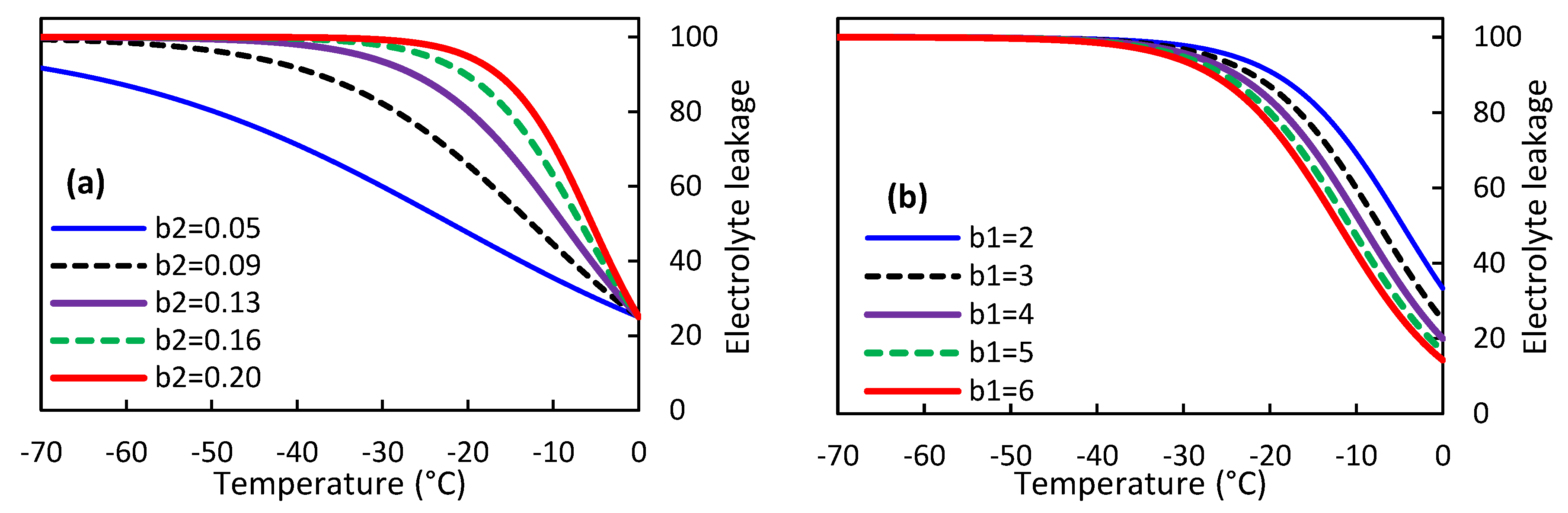
Figure 2.
Nonlinear regression modeling of olive electrolyte leakage characteristics at subzero temperatures (-50°C to 0°C) for pre, deep, and post-Dormancy stages.
Figure 2.
Nonlinear regression modeling of olive electrolyte leakage characteristics at subzero temperatures (-50°C to 0°C) for pre, deep, and post-Dormancy stages.
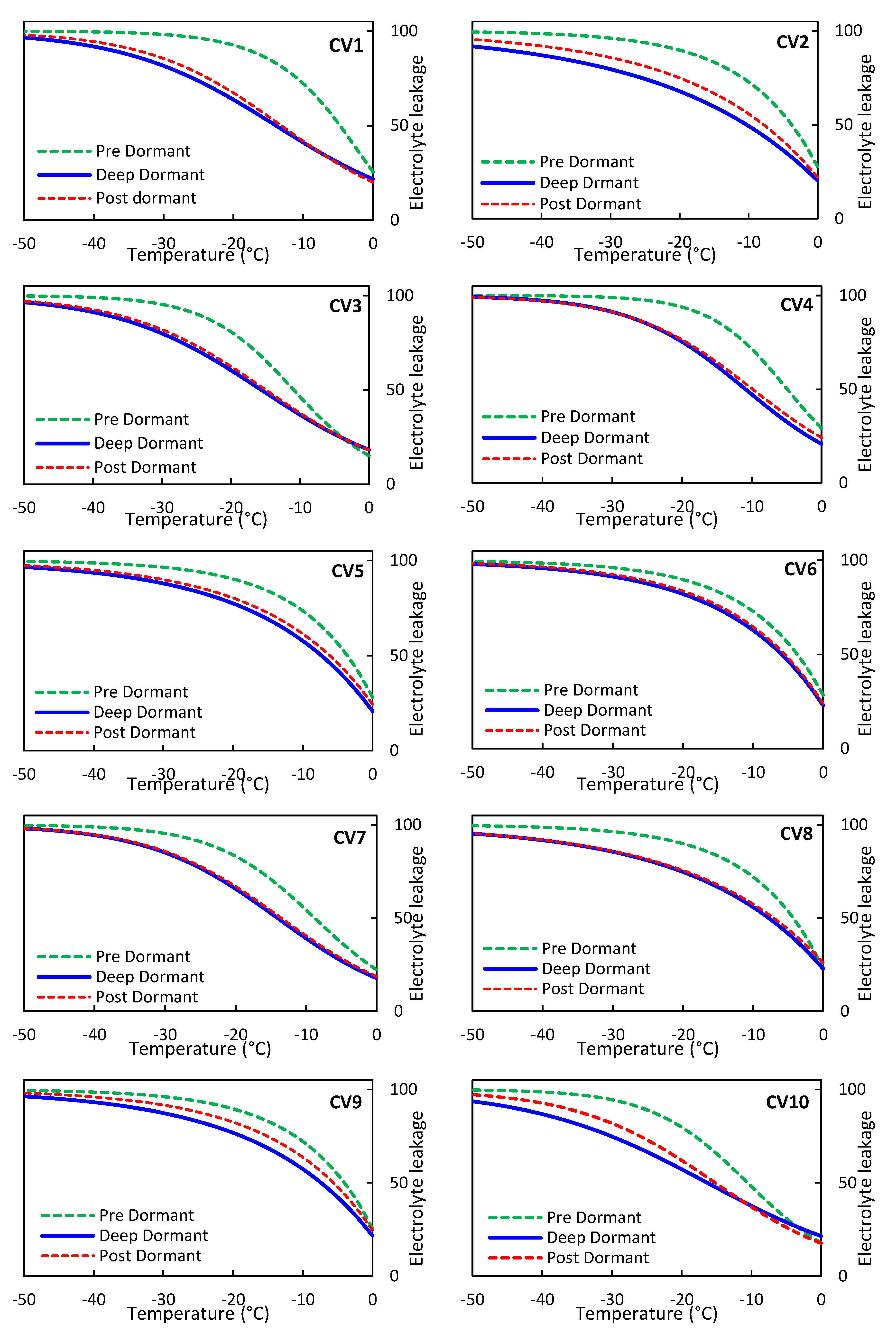
Figure 3.
Rate of change in olive EL at subzero temperatures (-50°C to 0°C) during pre, deep, and post-dormancy stages.
Figure 3.
Rate of change in olive EL at subzero temperatures (-50°C to 0°C) during pre, deep, and post-dormancy stages.
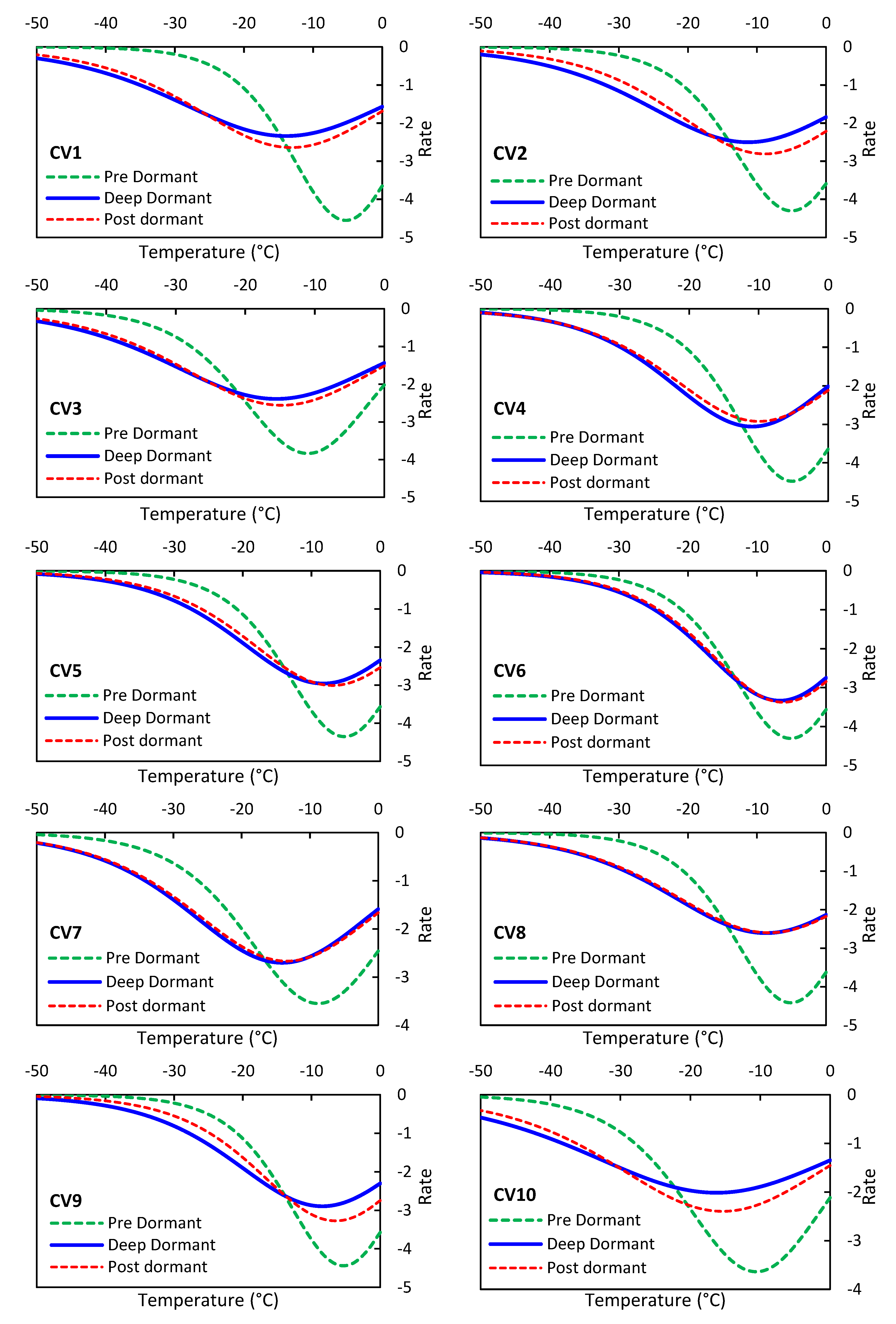
Figure 4.
the impact of altering the regression coefficients b1 and b2 in the M4 model on the vulnerability of olives to damage caused by freezing.
Figure 4.
the impact of altering the regression coefficients b1 and b2 in the M4 model on the vulnerability of olives to damage caused by freezing.
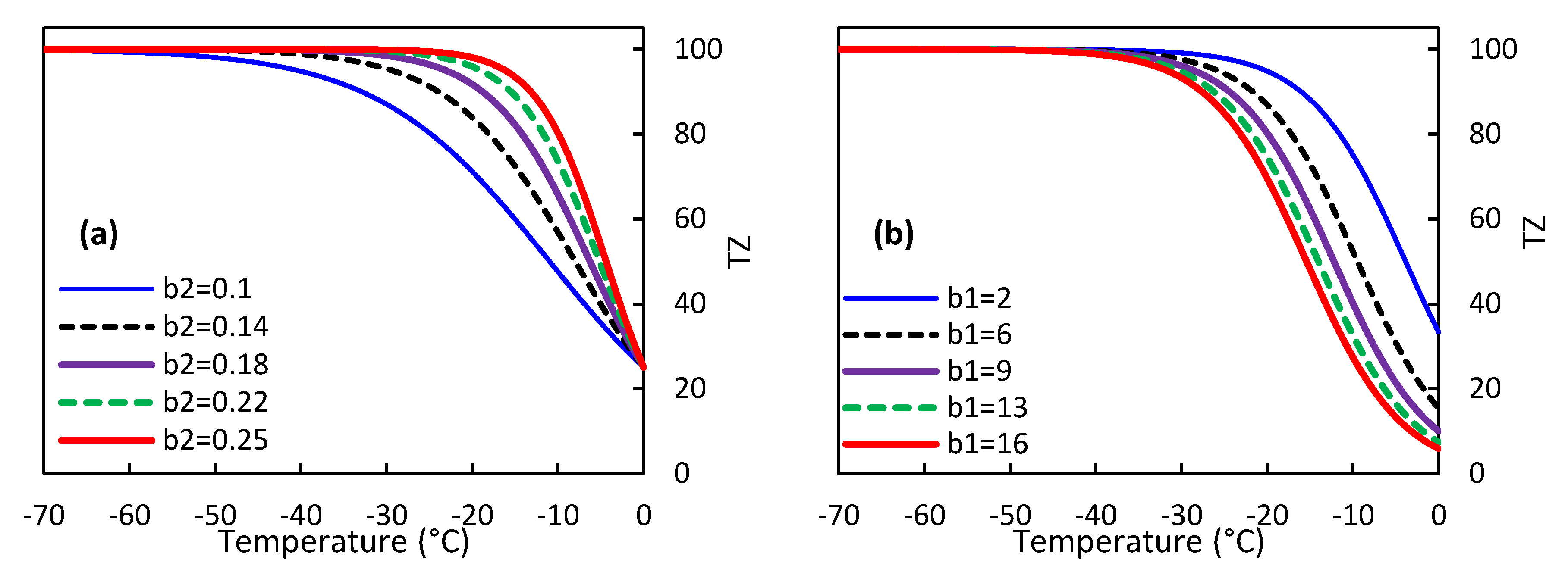
Figure 5.
the modeling of olive TZ characteristics at subzero temperatures ranging from -50°C to 0°C for pre, deep, and post-dormancy using nonlinear regression.
Figure 5.
the modeling of olive TZ characteristics at subzero temperatures ranging from -50°C to 0°C for pre, deep, and post-dormancy using nonlinear regression.
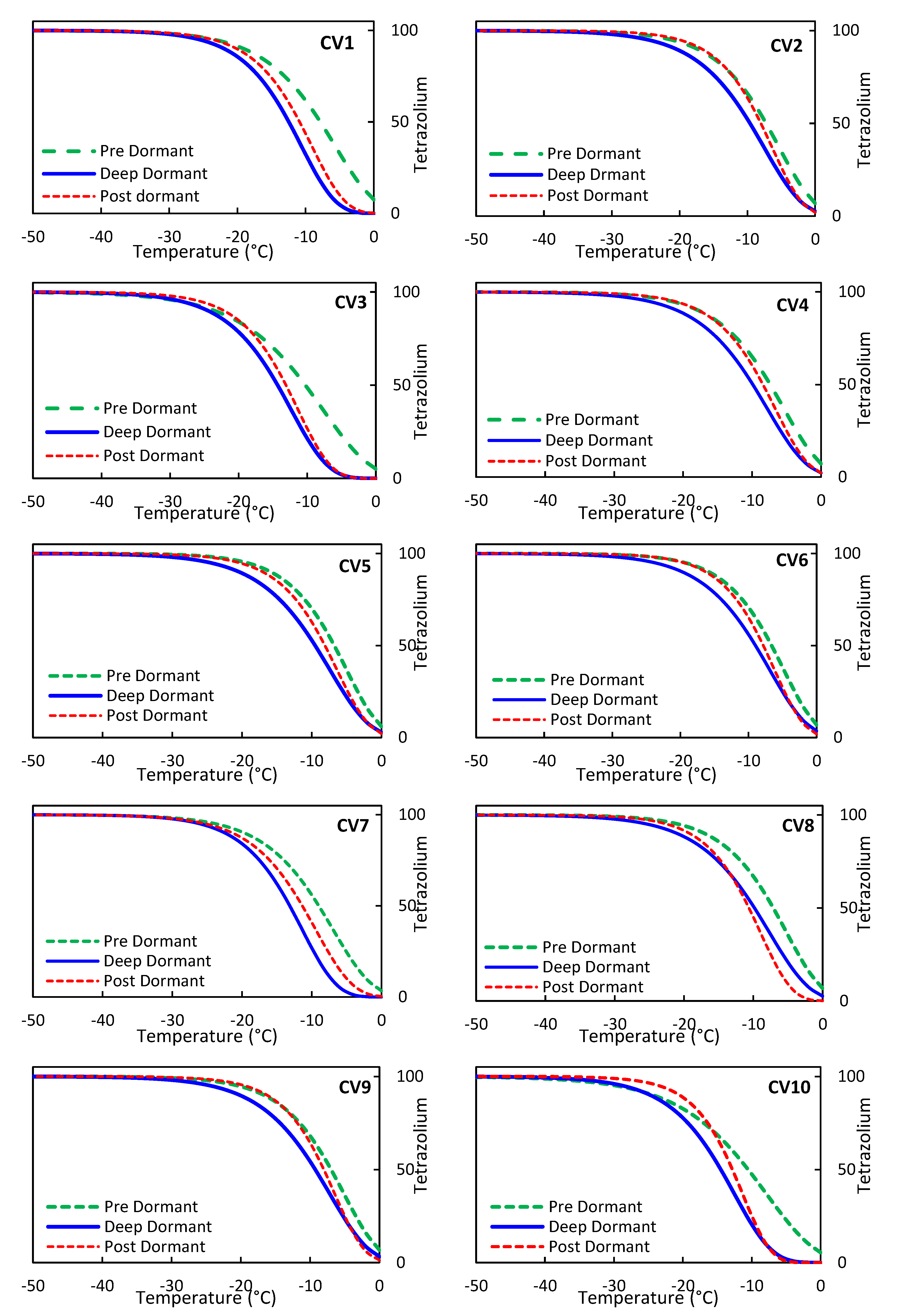
Figure 6.
Rate of changes in olive TZ during the stages of pre, deep, and Post-dormancy at temperatures below zero, ranging from -50°C to 0°C.
Figure 6.
Rate of changes in olive TZ during the stages of pre, deep, and Post-dormancy at temperatures below zero, ranging from -50°C to 0°C.
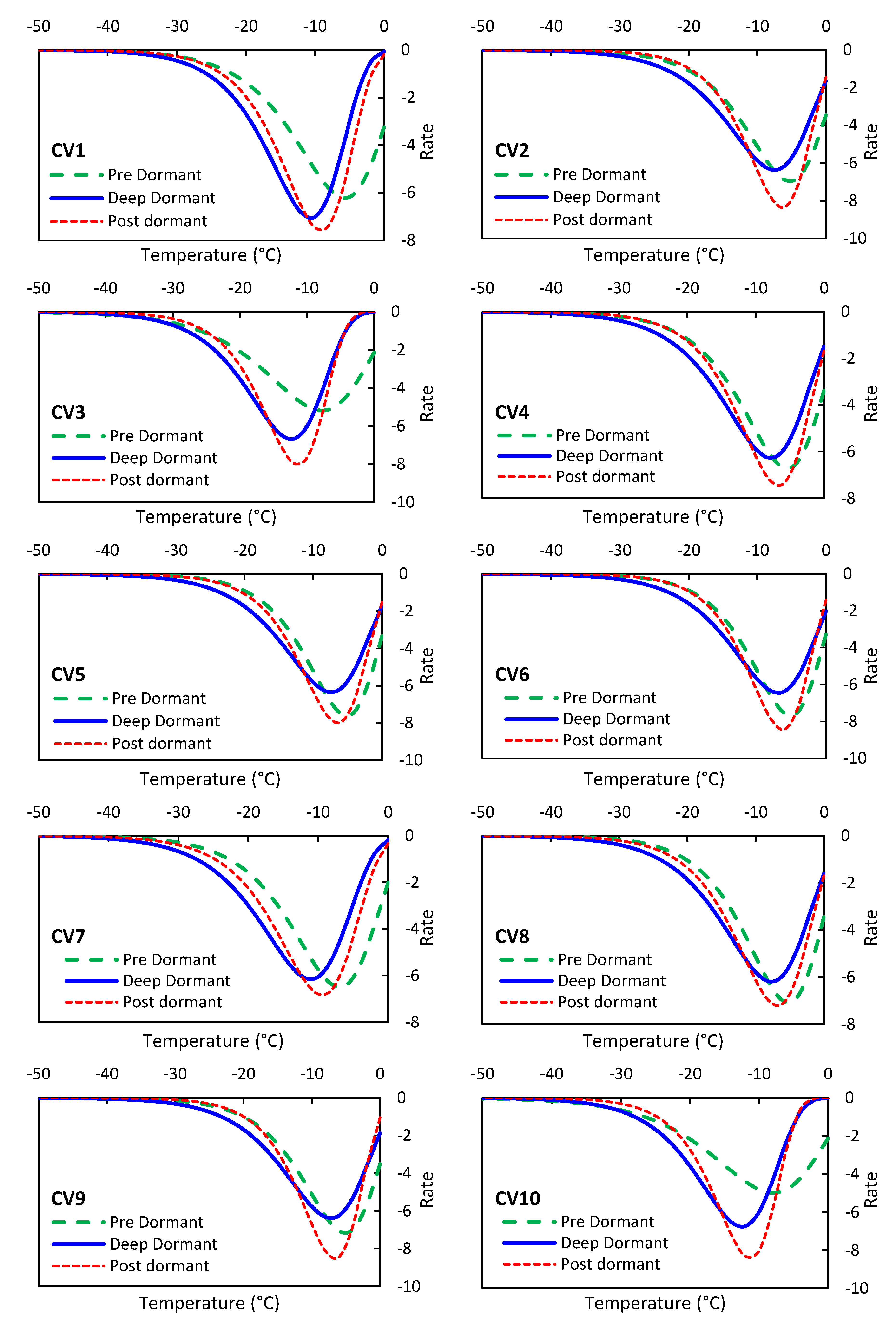

Table 1.
Matematical models to estimate freezing injuries on ten olive cultivars.
| Symbol | Form | Model | Name |
| EXP0 | M1 | Exponential model without LAG | |
| EXPLAG | M2 | Exponential model with LAG | |
| L2p | M3 | 2p-logistic model | |
| GOM | M4 | Gompertz model | |
| LOG | M5 | Logistic model | |
| GOM2 | M6 | Gompertz model 2 | |
| LOG2 | M7 | Logistic model 2 | |
| TPLOG | M8 | Two-pool logistic | |
| OPLOG | M9 | One-pool logistic | |
| MGOM | M10 | Modified Gompertz model | |
| RCD | M11 | Richard model | |
| ELM | M12 | Exponential-linear model | |
| OPG | M13 | One pool Gompertz | |
| RCD2 | M14 | Richard model 2 | |
| RCD3 | M15 | Richard model 3 | |
| RCD4 | M16 | Richard model 4 | |
| GOM3 | M17 | Gompertz model 3 | |
| GOM4 | M18 | Gompertz model 4 |
Table 2.
the RMSE values for EL estimation of eight out of the eighteen investigated NLR models, for different cultivars of olives.
Table 2.
the RMSE values for EL estimation of eight out of the eighteen investigated NLR models, for different cultivars of olives.
| CV1 | CV2 | CV3 | CV4 | CV5 | |||||||||||
| Pre | Deep | Post | Pre | Deep | Post | Pre | Deep | Post | Pre | Deep | Post | Pre | Deep | Post | |
| M2 | 7.53 | 5.14 | 5.01 | 8.47 | 4.52 | 5.22 | 8.68 | 5.36 | 6.89 | 7.2 | 4.89 | 5.03 | 7.23 | 5.22 | 7.07 |
| M3 | 8.5 | 4.37 | 3.49 | 9.06 | 4.84 | 6.03 | 4.89 | 3.96 | 5.39 | 8.04 | 3.5 | 5.45 | 7.95 | 6.77 | 8.44 |
| M4 | 7.79 | 4.62 | 3.95 | 8.48 | 4.56 | 5.49 | 6.34 | 4.47 | 5.87 | 7.39 | 3.75 | 4.93 | 7.37 | 5.94 | 7.72 |
| M5 | 8.5 | 4.37 | 3.49 | 9.06 | 4.84 | 6.03 | 4.89 | 3.96 | 5.39 | 8.04 | 3.5 | 5.45 | 7.95 | 6.77 | 8.44 |
| M6 | 7.79 | 4.62 | 3.95 | 8.48 | 4.56 | 5.49 | 6.34 | 4.47 | 5.87 | 7.39 | 3.75 | 4.93 | 7.37 | 5.94 | 7.72 |
| M8 | 8.46 | 4.38 | 3.3 | 9.04 | 4.84 | 6.03 | 3.6 | 3.64 | 5.21 | 8.02 | 3.48 | 5.45 | 7.88 | 6.78 | 8.45 |
| M10 | 7.79 | 4.62 | 3.95 | 8.48 | 4.56 | 5.49 | 6.34 | 4.47 | 5.87 | 7.39 | 3.75 | 4.93 | 7.37 | 5.94 | 7.72 |
| M14 | 7.79 | 4.3 | 3.4 | 8.45 | 4.57 | 5.49 | 3.82 | 3.76 | 5.41 | 7.31 | 3.5 | 4.93 | 7.22 | 5.95 | 7.72 |
| CV6 | CV7 | CV8 | CV9 | CV10 | |||||||||||
| Pre | Deep | Post | Pre | Deep | Post | Pre | Deep | Post | Pre | Deep | Post | Pre | Deep | Post | |
| M2 | 7.83 | 3.29 | 6.18 | 6.91 | 7.24 | 6.46 | 6.98 | 6 | 5.69 | 7.51 | 5.52 | 6.4 | 8.61 | 4.22 | 7.48 |
| M3 | 8.51 | 4.66 | 7.51 | 5.07 | 5.56 | 4.74 | 8.06 | 7.54 | 6.92 | 8.42 | 6.93 | 7.68 | 5.59 | 4.11 | 6.11 |
| M4 | 7.91 | 3.87 | 6.74 | 5.5 | 6.17 | 5.32 | 7.33 | 6.8 | 6.28 | 7.77 | 6.18 | 6.95 | 6.73 | 4.06 | 6.57 |
| M5 | 8.51 | 4.66 | 7.51 | 5.07 | 5.56 | 4.74 | 8.06 | 7.54 | 6.92 | 8.42 | 6.93 | 7.68 | 5.59 | 4.11 | 6.11 |
| M6 | 7.91 | 3.87 | 6.74 | 5.5 | 6.17 | 5.32 | 7.33 | 6.8 | 6.28 | 7.77 | 6.18 | 6.95 | 6.73 | 4.06 | 6.57 |
| M8 | 8.47 | 4.66 | 7.51 | 4.81 | 5.21 | 4.24 | 8.06 | 7.57 | 6.95 | 8.38 | 6.94 | 7.69 | 4.29 | 4.11 | 5.65 |
| M10 | 7.91 | 3.87 | 6.74 | 5.5 | 6.17 | 5.32 | 7.33 | 6.8 | 6.28 | 7.77 | 6.18 | 6.95 | 6.73 | 4.06 | 6.57 |
| M14 | 7.86 | 3.86 | 6.74 | 5.08 | 5.27 | 4.49 | 7.32 | 6.81 | 6.28 | 7.69 | 6.18 | 6.95 | 5.05 | 4.05 | 5.82 |
CV1 to CV10 are the olive cultivars, while Pre, Deep, and Post refer to the dormancy stages, and M2 to M14 are the NLR models (Table 1).
Table 3.
The statistical analysis results of the coefficients for the M3 model used to estimate EL based on sub-zero temperatures for all experimental cases.
Table 3.
The statistical analysis results of the coefficients for the M3 model used to estimate EL based on sub-zero temperatures for all experimental cases.
| CV1 | CV2 | ||||||
| Pre | Deep | Post | Pre | Deep | Post | ||
| Cofe. | 2.47**±0.41 | 3.62**±0.31 | 3.98**±0.28 | 2.63**±0.41 | 3.07**±0.28 | 2.67**±0.29 | |
| 0.18**±0.02 | 0.09**±0.01 | 0.11**±0.01 | 0.18**±0.02 | 0.10**±0.01 | 0.11**±0.01 | ||
| 0.87, 0.86 | 0.92, 0.92 | 0.96, 0.96 | 0.90, 0.90 | 0.92, 0.91 | 0.89, 0.89 | ||
| CV3 | CV4 | ||||||
| Pre | Deep | Post | Pre | Deep | Post | ||
| Cofe. | 5.60**±0.63 | 4.48**±0.30 | 4.51**±0.47 | 2.43**±0.38 | 3.81**±0.27 | 3.14**±0.33 | |
| 0.16**±0.01 | 0.10**±0.00 | 0.10**±0.01 | 0.18**±0.02 | 0.12**±0.01 | 0.12**±0.01 | ||
| 0.96, 0.96 | 0.97, 0.97 | 0.92, 0.91 | 0.88, 0.88 | 0.97, 0.97 | 0.92, 0.91 | ||
| CV5 | CV6 | ||||||
| Pre | Deep | Post | Pre | Deep | Post | ||
| Cofe. | 2.36**±0.36 | 2.65**±0.33 | 2.26**±0.34 | 2.50**±0.36 | 2.54**±0.20 | 2.32**±0.32 | |
| 0.18**±0.02 | 0.12**±0.01 | 0.12**±0.01 | 0.18**±0.02 | 0.14**±0.01 | 0.14**±0.01 | ||
| 0.88, 0.88 | 0.88, 0.87 | 0.81, 0.80 | 0.91, 0.91 | 0.96, 0.96 | 0.87, 0.86 | ||
| CV7 | CV8 | ||||||
| Pre | Deep | Post | Pre | Deep | Post | ||
| Cofe. | 3.50**±0.30 | 4.65**±0.56 | 4.38**±0.44 | 2.42**±0.38 | 2.48**±0.33 | 2.37**±0.29 | |
| 0.14**±0.01 | 0.11**±0.01 | 0.11**±0.01 | 0.18**±0.02 | 0.10**±0.01 | 0.10**±0.01 | ||
| 0.96, 0.96 | 0.90, 0.90 | 0.93, 0.92 | 0.88, 0.87 | 0.83, 0.82 | 0.85, 0.84 | ||
| CV9 | CV10 | ||||||
| Pre | Deep | Post | Pre | Deep | Post | ||
| Cofe. | 2.57**±0.36 | 2.64**±0.33 | 2.32**±0.32 | 4.62**±0.56 | 3.67**±0.30 | 4.70**±0.55 | |
| 0.18**±0.02 | 0.11**±0.00 | 0.13**±0.01 | 0.15**±0.01 | 0.08**±0.01 | 0.10**±0.01 | ||
| 0.92, 0.92 | 0.87, 0.86 | 0.86, 0.85 | 0.94, 0.93 | 0.90, 0.90 | 0.87, 0.86 | ||
Table 4.
The values of T50 and T90 for ten olive cultivars during three stages: pre-dormancy, deep dormancy, and post-dormancy.
Table 4.
The values of T50 and T90 for ten olive cultivars during three stages: pre-dormancy, deep dormancy, and post-dormancy.
| CV1 | CV2 | CV3 | |||||||
| Pre | Deep | Post | Pre | Deep | Post | Pre | Deep | Post | |
| T50 | -5.26 | -13.95 | -13.14 | -5.01 | -11.32 | -8.84 | -10.99 | -15.53 | -14.76 |
| T90 | -17.32 | -37.43 | -33.94 | -17.78 | -33.28 | -28.40 | -25.31 | -38.50 | -36.21 |
| CV4 | CV5 | CV6 | |||||||
| Pre | Deep | Post | Pre | Deep | Post | Pre | Deep | Post | |
| T50 | -5.14 | -10.92 | -9.94 | -5.21 | -8.29 | -6.95 | -5.11 | -6.69 | -6.21 |
| T90 | -17.41 | -28.87 | -28.73 | -17.83 | -26.86 | -25.22 | -17.87 | -23.15 | -22.47 |
| CV7 | CV8 | CV9 | |||||||
| Pre | Deep | Post | Pre | Deep | Post | Pre | Deep | Post | |
| T50 | -8.79 | -14.08 | -13.39 | -5.11 | -8.72 | -8.22 | -5.34 | -8.42 | -6.49 |
| T90 | -24.27 | -34.40 | -33.98 | -17.54 | -29.79 | -29.37 | -17.71 | -27.40 | -23.27 |
| CV10 | |||||||||
| Pre | Deep | Post | |||||||
| T50 | -10.58 | -16.26 | -15.36 | ||||||
| T90 | -25.68 | -43.53 | -38.28 | ||||||
Table 5.
the RMSE values for estimating TZ of eight out of the eighteen NLR models that were investigated, across various olive cultivars.
Table 5.
the RMSE values for estimating TZ of eight out of the eighteen NLR models that were investigated, across various olive cultivars.
| CV1 | CV2 | CV3 | CV4 | CV5 | |||||||||||
| Pre | Deep | Post | Pre | Deep | Post | Pre | Deep | Post | Pre | Deep | Post | Pre | Deep | Post | |
| M3 | 9.24 | 5.78 | 4.97 | 8.63 | 6.2 | 7.32 | 8.12 | 5.26 | 7.15 | 8.09 | 6.22 | 6.98 | 8.21 | 6.68 | 6.34 |
| M4 | 8.8 | 6.21 | 5.65 | 7.84 | 5.16 | 6.27 | 8.34 | 6.22 | 7.86 | 7.22 | 5.2 | 5.93 | 7.33 | 5.72 | 5.6 |
| M5 | 9.24 | 5.78 | 4.97 | 8.63 | 6.2 | 7.32 | 8.12 | 5.26 | 7.15 | 8.09 | 6.22 | 6.98 | 8.21 | 6.68 | 6.34 |
| M6 | 8.8 | 6.21 | 5.65 | 7.84 | 5.16 | 6.27 | 8.34 | 6.22 | 7.86 | 7.22 | 5.2 | 5.93 | 7.33 | 5.72 | 5.6 |
| M7 | 9.24 | 5.78 | 4.97 | 8.63 | 6.2 | 7.32 | 8.12 | 5.26 | 7.15 | 8.09 | 6.22 | 6.98 | 8.21 | 6.68 | 6.34 |
| M10 | 8.8 | 6.21 | 5.65 | 7.84 | 5.16 | 6.27 | 8.34 | 6.22 | 7.86 | 7.22 | 5.2 | 5.93 | 7.33 | 5.72 | 5.6 |
| M13 | 8.8 | 6.21 | 5.65 | 7.84 | 5.16 | 6.27 | 8.34 | 6.22 | 7.86 | 7.22 | 5.2 | 5.93 | 7.33 | 5.72 | 5.6 |
| M14 | 8.8 | 5.75 | 4.95 | 7.83 | 5.16 | 6.21 | 8.09 | 5.15 | 7.13 | 7.22 | 5.2 | 5.93 | 7.27 | 5.73 | 5.57 |
| CV6 | CV7 | CV8 | CV9 | CV10 | |||||||||||
| Pre | Deep | Post | Pre | Deep | Post | Pre | Deep | Post | Pre | Deep | Post | Pre | Deep | Post | |
| M3 | 8.52 | 6.47 | 4.6 | 8.22 | 5.4 | 4 | 8.18 | 6.68 | 13.2 | 8.12 | 6.59 | 7.49 | 8.73 | 5.84 | 10.8 |
| M4 | 7.69 | 5.35 | 4.53 | 8.52 | 6.67 | 4.83 | 7.23 | 5.69 | 15.33 | 7.11 | 5.53 | 7.45 | 8.93 | 7.03 | 10.76 |
| M5 | 8.52 | 6.47 | 4.6 | 8.22 | 5.4 | 4 | 8.18 | 6.68 | 13.2 | 8.12 | 6.59 | 7.49 | 8.73 | 5.84 | 10.8 |
| M6 | 7.69 | 5.35 | 4.53 | 8.52 | 6.55 | 4.83 | 7.23 | 5.69 | 15.33 | 7.11 | 5.53 | 7.45 | 8.93 | 7.03 | 10.76 |
| M7 | 8.52 | 6.47 | 4.6 | 8.22 | 5.4 | 4 | 8.18 | 6.68 | 13.2 | 8.12 | 6.59 | 7.49 | 8.73 | 5.84 | 10.8 |
| M10 | 7.69 | 5.35 | 4.53 | 8.52 | 6.55 | 4.83 | 7.23 | 5.69 | 15.33 | 7.11 | 5.53 | 7.45 | 8.93 | 7.03 | 10.76 |
| M13 | 7.69 | 5.35 | 4.53 | 8.52 | 6.55 | 4.83 | 7.23 | 5.69 | 15.33 | 7.11 | 5.53 | 7.45 | 8.93 | 7.03 | 10.76 |
| M14 | 7.55 | 5.35 | 4.38 | 8.2 | 5.4 | 3.99 | 7.23 | 5.69 | 11.33 | 7.11 | 5.53 | 7.11 | 8.7 | 5.44 | 10.8 |
Table 6.
the statistical analysis outcomes of the coefficients for the M4 model that was utilized to calculate TZ using sub-zero temperatures for all experimental cases.
Table 6.
the statistical analysis outcomes of the coefficients for the M4 model that was utilized to calculate TZ using sub-zero temperatures for all experimental cases.
| CV1 | CV2 | ||||||
| Pre | Deep | Post | Pre | Deep | Post | ||
| Cofe. | 2.58**±0.37 | 8.24**±1.59 | 6.39**±1.00 | 2.68**±0.36 | 3.79**±0.40 | 3.59**±0.55 | |
| 0.17**±0.02 | 0.20**±0.02 | 0.20**±0.01 | 0.19**±0.02 | 0.18**±0.01 | 0.22**±0.02 | ||
| 0.93, 0.92 | 0.97, 0.97 | 0.97, 0.97 | 0.94, 0.94 | 0.98, 0.98 | 0.97, 0.97 | ||
| CV3 | CV4 | ||||||
| Pre | Deep | Post | Pre | Deep | Post | ||
| Cofe. | 2.98**±0.42 | 9.81**±2.09 | 10.51**±2.89 | 2.63**±0.32 | 3.80**±0.40 | 3.81**±0.48 | |
| 0.14**±0.01 | 0.19**±0.02 | 0.21**±0.02 | 0.18**±0.02 | 0.17**±0.01 | 0.20**±0.01 | ||
| 0.93, 0.92 | 0.96, 0.96 | 0.95, 0.94 | 0.95, 0.95 | 0.98, 0.97 | 0.97, 0.97 | ||
| CV5 | CV6 | ||||||
| Pre | Deep | Post | Pre | Deep | Post | ||
| Cofe. | 2.80**±0.34 | 3.58**±0.40 | 3.84**±0.47 | 2.67**±0.36 | 3.34**±0.34 | 3.98**±0.40 | |
| 0.21**±0.02 | 0.17**±0.01 | 0.21**±0.01 | 0.20**±0.02 | 0.18**±0.01 | 0.22**±0.01 | ||
| 0.96, 0.96 | 0.97, 0.97 | 0.98, 0.97 | 0.95, 0.95 | 0.97, 0.97 | 0.98, 0.98 | ||
| CV7 | CV8 | ||||||
| Pre | Deep | Post | Pre | Deep | Post | ||
| Cofe. | 3.38**±0.55 | 9.94**±2.03 | 5.87**±0.47 | 2.69**±0.34 | 3.66**±0.41 | 7.24*±2.81 | |
| 0.18**±0.02 | 0.20**±0.02 | 0.19**±0.01 | 0.19**±0.02 | 0.17**±0.01 | 0.22**±0.04 | ||
| 0.94, 0.93 | 0.97, 0.97 | 0.99, 0.99 | 0.95, 0.95 | 0.97, 0.97 | 0.88, 0.88 | ||
| CV9 | CV10 | ||||||
| Pre | Deep | Post | Pre | Deep | Post | ||
| Cofe. | 2.69**±0.34 | 3.44**±0.37 | 4.38**±0.62 | 2.92**±0.43 | 9.98**±2.17 | 16.07*±6.00 | |
| 0.19**±0.02 | 0.17**±0.01 | 0.23**±0.02 | 0.14**±0.01 | 0.18**±0.02 | 0.25**±0.03 | ||
| 0.95, 0.95 | 0.97, 0.97 | 0.98, 0.98 | 0.91, 0.91 | 0.96, 0.96 | 0.97, 0.96 | ||
Table 7.
the T50 and T90 values based on TZ for ten different olive cultivars across three stages, namely pre, deep, and post-dormancy stages.
Table 7.
the T50 and T90 values based on TZ for ten different olive cultivars across three stages, namely pre, deep, and post-dormancy stages.
| CV1 | CV2 | CV3 | |||||||
| Pre | Deep | Post | Pre | Deep | Post | Pre | Deep | Post | |
| T50 | -7.84 | -12.51 | -10.88 | -7.15 | -9.58 | -7.91 | -10.31 | -14.36 | -13.00 |
| T90 | -18.98 | -22.33 | -20.02 | -17.11 | -20.46 | -16.21 | -23.69 | -24.74 | -21.64 |
| CV4 | CV5 | CV6 | |||||||
| Pre | Deep | Post | Pre | Deep | Post | Pre | Deep | Post | |
| T50 | -7.37 | -9.92 | -8.43 | -6.89 | -9.53 | -8.13 | -6.89 | -9.01 | -7.86 |
| T90 | -17.71 | -20.98 | -17.74 | -16.01 | -20.45 | -16.82 | -15.93 | -19.77 | -16.08 |
| CV7 | CV8 | CV9 | |||||||
| Pre | Deep | Post | Pre | Deep | Post | Pre | Deep | Post | |
| T50 | -8.98 | -13.24 | -11.38 | -7.09 | -9.85 | -8.64 | -6.99 | -9.29 | -8.18 |
| T90 | -19.66 | -24.50 | -21.53 | -16.88 | -21.05 | -18.25 | -16.65 | -20.15 | -16.31 |
| CV10 | |||||||||
| Pre | Deep | Post | |||||||
| T50 | -10.59 | -14.43 | -12.85 | ||||||
| T90 | -24.49 | -24.68 | -21.08 | ||||||
Disclaimer/Publisher’s Note: The statements, opinions and data contained in all publications are solely those of the individual author(s) and contributor(s) and not of MDPI and/or the editor(s). MDPI and/or the editor(s) disclaim responsibility for any injury to people or property resulting from any ideas, methods, instructions or products referred to in the content. |
© 2023 by the authors. Licensee MDPI, Basel, Switzerland. This article is an open access article distributed under the terms and conditions of the Creative Commons Attribution (CC BY) license (http://creativecommons.org/licenses/by/4.0/).
Copyright: This open access article is published under a Creative Commons CC BY 4.0 license, which permit the free download, distribution, and reuse, provided that the author and preprint are cited in any reuse.


