
Submitted:
26 April 2023
Posted:
27 April 2023
You are already at the latest version
Abstract
Being one of the most critical phases of a flight, landing deserves specific attention, especially when the aircraft is subject to external disturbances such as wind. A notable concern associated with touchdown events, especially when crosswind is present is tire wear. This work is aimed first at developing a nonlinear flight simulator able to handle the entire landing maneuver in non-null wind conditions, considering the airborne phase, ground run, and the transition between them. Then, the simulator is included in an optimal process to define the landing technique associated with the minimum tire wear. The methodology is tested in a simulation environment with a realistic model of a reference aircraft, showing that a significant reduction of tire wear can be obtained by optimizing the sideslip angle at touchdown and the lateral-directional controls after the airplane touches the runway with both legs of the main landing gear.
Keywords:
Landing
; Flight simulation
; Tire wear
; Optimization
; Crosswind
; Nonlinear flight dynamics
; Trim
; Ground-contact detection
1. Introduction
Landing is one of the most critical phases of a flight because the aircraft is flying at low altitudes and low speeds while external disturbances, most notably wind, may bring the aircraft into dangerous conditions due to the proximity of the terrain [1]. Notwithstanding this fact, the safety of landing maneuvers is ensured by effective and consolidated airport procedures, improved knowledge of weather conditions, and the use of automatic controls for approach and landing.
In addition to all considerations about safety, during the touchdown phase, the forces generated by the contact-impact of the landing gear on the runway are the cause of fatigue on the airframe structural subcomponents and significant wear of tires.
The tire wear is even more significant when the airplane lands in crosswind conditions. In fact, during the airborne phase, the airplane cannot be simultaneously aligned with the runway and in a symmetric flight regime, hence, it will initially touch the ground with only one leg of the main gear and with an asymmetric attitude, undergoing a lateral drift of the wheels. Clearly, in this scenario, techniques aimed at reducing tire wear may be beneficial for airplane operations and maintenance.
The aim of this work is twofold: firstly, to develop a landing maneuver simulator for a fixed-wing aircraft to be employed in a variety of touchdown scenarios, with special emphasis on crosswind conditions, and secondarily, to study the optimal landing maneuver associated with minimum tire wear.
The definition of optimal trajectories through the minimization of a suitable cost function is a long-standing topic in the literature related to flying machines and many examples of different optimization processes are already available [2,3,4,5].
Landing simulation is widely discussed in the literature. In fact, one of the most challenging aspects of modern flight simulators is to reproduce the aircraft-ground interaction during landing, in order to allow the simulation of such a complex maneuver, especially in non-null wind conditions.
In order to formulate a simulator able to handle landing maneuvers, considering both airborne phase and ground run, one has to develop and integrate multiple models for each subsystem, i.e. the model of the aircraft, the model of the landing gear, including tire dynamics and shock absorbers, and the model of the forces associated to the contact among the tire and the runway. The integrated dynamics of the system should also be linked to an algorithm for detecting the contact between a single leg of the landing gear and the ground.
As far as the landing gear dynamics is concerned, several levels of detail may be considered. Dreier [6] proposes a simplified landing gear linear model, in which tires and shock absorbers are modeled as linear spring-damper systems, with a preloaded force to capture the gas pressure preload. Evans [7] applied this simplified linear model to a real-time flight simulator capable of simulating landing conditions, whereas Wang and Holzapfel [8] consider a rigid tire and a linear elastic shock absorber to study abnormal runway contact conditions.
Even though linear approximations are typically employed for modeling all landing gear elements, it is certainly possible to improve the accuracy of the overall modeling including the nonlinear behavior of some subcomponents, such as shock absorbers, without increasing the overall complexity level of the model. Daniels [9] developed a complete nonlinear simulator of a telescopic oleo-pneumatic landing gear, including nonlinearities arising from polytropic gas compression, oil damping, stroke-dependent discharge coefficient, and internal stick friction. This highly detailed model was validated against experimental data acquired from an A-6 aircraft landing gear.
The interaction between tires and runway and the modeling of normal and in-plane reaction forces represent a point that deserves specific attention.
Different models for tire dynamics and for the determination of the contact point are analyzed in Yang et al. [10]. The authors concluded that even simple models with low computational costs may provide for good approximations in the case of contact over flat surfaces, even if using more complex models improves the estimation of the tire deformations.
Barnes and Yager [11] developed very effective longitudinal and lateral friction models, extended to large tire yaw angles, which take into account runway conditions (such as dry, wet, flooded surface), aircraft velocity, and simple tire psychical properties. Sice it represent a good compromise between complexity and reliability, this model is suitable for online computations, and was subsequently used in Vechtel [12], Vechtel et al. [13] for landing simulations.
Standalone evaluation of landing gear performance may also consider tire shimmy, i.e. an oscillatory phenomenon due to the interaction between tire footprint modification and the wheel plane. Shepherd et al. [14]) considered this phenomenon through a procedure featuring a much higher level of complexity.
Aircraft and landing gear dynamics shall be integrated to perform a complete landing simulation. This fact emphasizes, even more, the need for finding a good compromise between modeling complexity and computational costs, as witnessed by the works of Evans [7], Evans et al. [15], Lei et al. [16] and Wen et al. [17]. In all these works, linear or nonlinear dynamical models of the aircraft are integrated with linearized landing gear dynamics, possibly including simple algorithms for ground contact detection.
Given the scope of the present work, the last aspect to consider is the estimation of tire wear, which represents a problem of great interest for civil aviation [18]. Notwithstanding the apparent complexity of this subject, tire wear is widely studied in many applications, typically connected with the automotive sector, and some simple but effective modeling strategies are already available in the literature, [19,20,21].
Inspired by the previous literature, in this work, a simulator, able to handle the entire landing of a generic aircraft including the airborne phase and ground run, is developed paying attention to the compromise between model complexity and result accuracy. In particular, a 6-DoF nonlinear model of aircraft, of greater complexity wrt. the one previously proposed by the authors for terminal maneuvers [2,22] and based on the theoretical framework typically adopted in the anlysis flight trajectories [4,23], is integrated with a nonlinear landing gear system that considers a linearized dynamics tire and a nonlinear model for the forces exerted by the shock absorbers. The dynamics of the tires is triggered by a ground-contact detection algorithm that works independently on each leg of the landing gear to suitably capture the behavior of the system in case of asymmetric landing scenarios. The tool is then included in an optimization algorithm aimed at evaluating the landing maneuver associated with the minimum tire wear.
The paper is organized according to the following plan. Section 2 deals with the definition of the simulator and considers the modeling and integration of aircraft, tire and shock absorber subsystems, and the algorithm for ground contact detection. The final part of this section is dedicated to the definition of the reference airplane model, used in this work, whose data are fully reported in Appendix A. In Section 3 the problem of airplane trim for non-null wind conditions is analyzed. Section 4 deals with the estimation of tire wear during touchdown and with its minimization through the optimization of the landing technique. The results of the optimization of the landing in crosswind conditions for minimum tire wear are reported in Section 5. Finally, Section 6 summarizes the main findings of this work and offers some insights on possible improvements and future developments.
2. Simulation model
In order to simulate and analyze the airplane landing in crosswind conditions, it is necessary to suitably model the system dynamics during the airborne, touchdown, and ground roll phases, considering the impact of the wind. The airplane is modeled as a rigid body in a three-dimensional domain, whereas the related aerodynamic forces and moments are linearized about a reference condition and rendered through the classical stability and control derivatives, as detailed in Section 2.1. A conventional tricycle landing gear with oleo-pneumatic shock absorbers is linked to the airplane model, as detailed in Section 2.2). Finally, the details of the reference aircraft model are reported in Paragraph 2.3.
2.1. Model of the aircraft
The airplane is modeled as a rigid body in three-dimensional space. To suitably consider the impact of crosswind and highlight all possible couplings between longitudinal and lateral-directional dynamics, the fully non-linear form of the equations of motion for rigid bodies is preferred.
As commonly done, we write the equations of motion in the body frame (), which is defined as a frame attached to the aircraft in its center of gravity, with unit vectors , , coincident respectively with the roll (pointing to the aircraft nose), pitch (pointing to the right wing) and yaw (pointing to the down-side) axes. Unit vectors , and define the symmetry plane of the aircraft. The local horizon frame (NED or is again attached to the aircraft center of gravity, and its unit vectors , , are constantly pointing towards the local North, local East, and Down (i.e. towards the center of the earth) directions. The three-dimensional rotation that transforms triad into triad is handle through the Euler angles of sequence 3–2–1, i.e. heading , pitch and roll , organized in vector . The associated rotation tensor has components in equal to
The navigational frame is parallel to the NED frame but its origin is on the runway threshold. Finally, point indicates the projection of the airplane center of gravity G on the ground along the third unit vector of NED frame itself.
The equations of motion, expressed in barycentric body frame (), read
where the superscript indicates that the components of the vector are expressed in the body frame. In Eq. (2), m is the mass of the aircraft, is the inertia tensor expressed with respect to the center of gravity, is linear velocity, and the angular velocity. The terms , , indicate, respectively, aerodynamic, gravity and reaction forces, and , indicate aerodynamic and reaction moments about the center of gravity G. The gravitational force in the body frame is easily expressed as
while the moment of the gravitational force about the center of gravity is null by definition.
The model of the aerodynamic forces and moments are linearized about a suitable reference condition and rendered through the stability and control derivatives. As usual, they are expressed in terms of linear and angular velocities, deflections of the control surfaces, thrust throttle and rate of the linear velocities. The effect of the wind speed should be also included in the modeling of aerodynamics. To this end, we may introduce the vectorial relationship among ground speed , wind speed and the airspeed ,
As a founding hypothesis, the wind is considered constant over time and uniform over space.
Accordingly, aerodynamic forces and moments are
where denotes values associated with the reference conditions, while throttle position and elevator , aileron and rudder deflections are collected in array . As a convention, is positive for upwards elevator deflection (positive pitching moment), is positive for right aileron upwards deflection (positive rolling moment) and is positive for leftwards rudder deflection (negative yawing moment). Finally, and represent the classical aerodynamic stability and control derivatives, taken with respect to a generic variable .
Reaction forces and moments are only present when the aircraft is in contact with the ground, and their expression will be detailed in Section 2.2.
Finally, the evolution in time of Euler angles is described by
where tensor is defined as
The position of the aiplane center of gravity in the navigational frame can be integrated along with Eq. (2) and (7), through the knowledge of its derivative
Notice that the third component of corresponds to the opposite of the airplane altitude. Such information will be used when it comes to defining the algorithm for tire-wheel contact detection.
2.2. Model of the landing gear
The interaction of the aircraft with the ground is rendered through a simple model of the landing gear linked with an algorithm to determine whether one or more landing gear wheels be in contact with the ground.
In order to have a simple but still accurate modeling, the following assumptions are made:
- Only tricycle landing gears are considered, with oleo-pneumatic shock absorbers on main and nose gears (one per leg);
- The direction of the shock absorber deflection is always parallel to the axis;
- Independently of the number of wheels on each landing gear leg, an equivalent single–tire–per–leg is considered. Furthermore, the wheel axle is located at the free end of the shock absorber;
- Steering capability of the nose gear is not modeled;
- The rolling dynamics of tires and spin-up loads are neglected;
- A flat and steady Earth is considered. Additionally, the landing surface does not move and is horizontal.
To easily describe ground contact dynamics, as done by Lei et al. [16], the strut and the tire reference frames are introduced.
The Strut frame origin is located at the point on which the shock absorber is linked to the fuselage. Frame is obtained by translating frame . The Tire frame origin is located at the geometric center of the wheel. Unit vectors and define a plane parallel to the Earth’s surface, while points towards the center of the Earth. As no tire steering angle is considered, remains parallel to the projection of on the Earth’s tangent plane, with forming a right-hand triad. Figure 1 schematically shows both frames and the related variables of interest.
2.2.1. Tire model
Tire dynamics is included in the model through a straightforward mass-spring-damper system, whose equivalent stiffness and equivalent damping are termed and respectively. As suggested by Yang et al. [10], such a simple model represents a reasonable solution to model the contact between wheels and ground, when irregularities on the pavement are neglected, providing for a good balance between modeling complexity and quality of the results. Figure 2 reports a sketch of the tire model.
The vertical force exerted on the tire contact point C, expressed in tire frame , is
where is tire deflection and its time derivative. The force acts parallel to the third unit vector of the tire frame , and in opposite direction.
2.2.2. Shock absorber model
An equivalent single-orifice shock absorber model is employed through a non-linear preloaded spring-damper system. The elastic and damping force can be accordingly expressed as
where is the absorber stroke, is its rate, is the cylinder preload pressure (internal pressure when ), is the cross section area of the cylinder, is the shock absorber internal volume when , is gas (air or nitrogen) polytropic coefficient, is oil density, is the orifice discharge coefficient and is the equivalent orifice section.
Equations (10a) show that, even for , the shock absorber exerts an internal force due to the preload pressure , equal to . When the force applied at the strut exceeds the preload force, the strut begins to compress.
2.2.3. Ground contact detection
Landing simulations require the detection of the instants in which each tire touches the ground or rebounds. The contact condition is formulated similarly to Lei et al. [16].
The position of the contact point for the undeformed tire with respect to the airplane center of gravity is given by
where is the position of point C respect to the wheel center, is the position of the wheel center respect to the point where the strut is attached to the airplane, while is the position of respect the center of gravity G.
Assuming a rigid airplane, the components of and in the body frame are readily obtained from the geometry of the airplane, whereas the position of the contact point C with respect to the wheel center is readily defined in tire coordinates as
where is the undeformed tire radius. Notice also that , since tire and NED frames are parallel.
The components in the NED frame of point C are readily available through
in which tensor has been used for transforming the components of and from reference to .
Finally, the distance L between the contact point on the wheel and the ground along the third axis of the NED frame can be easily computed through the following scalar product
where is the altitude of the airplane, which is computed integrating Eq. (8).
The tire has touched the ground when L becomes negative. When this condition is triggered, landing gear dynamics start to act.
2.2.4. Ground contact forces and moments
Once the aircraft has touched the ground, the reaction forces on the contact point arise. Each landing gear contact point generates three forces, which are the normal force, acting perpendicularly to the ground, and two in-plane forces due to friction, acting parallel to the ground surface. Associated with the reaction forces, their moments with respect to the aircraft center of gravity are considered as well. Assuming the deformation of the tire negligible, the expressions of reaction forces and moments expressed in the body frame are
2.3. Reference airplane definition
A flight mechanics model of a realistic airplane, inspired by the Lockheed Jetstar, has been used for the numerical analyses of this work. The aerodynamic data were extracted from already published NASA reports, [24,25,26], while realistic landing gear properties, including shock absorber and tire, were defined following design guidelines provided by Roskam [27], Torenbeek [28] and Currey [29]. Finally, real tire data were retrieved from Goodyear’s aviation tires catalog, [30]. A comprehensive list of the reference aircraft data is provided in Appendix A.
3. Airplane trim in non-null horizontal wind conditions
Null wind conditions are typically assumed in the analysis of the trim of flying systems (see [31] and reference therein). In this work, we extend such treatment to the case of steady wind.
Let us consider the nonlinear equations of motion for a rigid aircraft, Eq. (2). A trimmed flight is a regime in which the linear and angular velocity vector, viewed in the body frame, and are constant for constant controls , i.e.
The trim problem hence consists in finding, if any, the constant vectors , and along with the evolution of the Euler angles , not necessarily constant, which satisfy the nonlinear equations of motion in Eq. (2).
Trim analysis for null wind conditions leads to the fact that trajectories featuring angular velocity null or constant and parallel to gravity are trimmed. Consequently, all rectilinear flight regimes are trimmed, as well as all steady turning flights and helices, with the latter being the most generic trimmed conditions, as noticed by De Marco et al. [31]. For non-null wind conditions, as we will see in the following paragraphs, the set of flight regimes that can be trimmed is narrower.
3.1. Non-null wind condition
Let us now introduce wind velocity in the NED frame as
where and are the components blowing respectively from the south towards the north and from the west towards the east, and represent the horizontal wind. Component is the vertical wind, positive if “up-down”. Moreover, we assume that the wind velocity in the NED frame is constant in time and uniform over space.
In order to compute the impact of the wind on the aerodynamic forces and moments, one has to change refer to the wind components in the body frame, which can be computed easily through the change of basis as
The three components of in the body frame are named respectively tail-wind positive if towards airplane nose, cross-wind positive if towards the right-side of the airplane and normal wind positive if towards the airplane downside.
Equations (2b), (5b) and (18) can be combined, and evaluated for null reaction forces and moments, under the hypothesis of trimmed regime Eq. (16), yielding
In Eq. (19), the superscript has been removed to simplify the notation. Clearly, all terms in Eqs. (19) but the gravitational ones are constant by definition and, hence, in order to verify the equality also and the components of the wind in body frame must be constant as well. By simply looking at the definitions of the rotation tensor and the wind velocity , it is simple to verify that this happens in two cases:
- For a generic , all Euler angles are constant, ;
- For a pure vertical wind, i.e. , roll and pitch angles are constant, .
As a first remark, notice that the conditions in the second case, associated with a pure vertical wind, are the same as the usual trim problem for null wind conditions. This implies that the possible trim conditions associated with pure upward or downward wind are identical to the usual case with null wind. A notable flight trajectory that satisfies the trim equation, eq. (19), for pure vertical upward wind is the ascending helix, which is exploited by gliders to gain height thanks to vertical wind flow.
On the other hand, the case with a generic wind, including horizontal wind components, i.e. cross- and tail-wind, admits only rectilinear flights. This fact is simple to be demonstrated by noticing that constant Euler angles () are needed to have constant rotation tensor and hence a constant product in Eq. (19b). Looking back to the kinematic relationship in Eq. (7), it is immediate to notice that the conditions imply necessarily a null angular velocity .
In this case, which is of interest for this work, the trim equations in Eq. (19) reduce to the straightforward equilibrium among aerodynamic and gravitational forces and moments.
3.2. Trim problem solution determination for non-null horizontal wind
The non-linear trim problem solution can be found looking for the set of linear and angular velocities, control inputs and Euler angles that satisfy Eq. (19). If horizontal wind components are considered, as demonstrated in Paragraph 3.1, this solution exists only if and constant Euler angles. Consequently, the array of the problem unknowns consists of 10 elements and is defined as
where is the vector with the constant Euler angles.
The nonlinear trim problem can be formalized as
Along with the equilibrium of forces and moments in Eqs. (21a) and (21b), Eq. (21c) is considered to impose a specific trimmed rectilinear trajectory through a specific value of . In landing, for example, the velocity in NED frame is dictated by the airplane approach velocity and the glide slope of the trajectory. Finally, Eq. (21d), is the classical piloting condition and refers to the choices that the pilot follows during the trimmed regime in terms of the variables of the lateral-direction plane. The piloting condition is formulated by fixing one among the side-slip angle , the aileron deflection , the rudder deflection , the roll angle , or the heading angle , to a predefined value. Dealing with landing with horizontal wind, the piloting condition can be set so as to specify a desired landing technique, such as
- : fly the aircraft without deflecting the rudder;
- or : fly the aircraft keeping zero sideslip angle (crabbed flight);
- : fly the aircraft aligning heading to ground track orientation (steady sideslipped flight)
The conditions defined in the last two bullet points, are commonly used during crosswind approaches and landings and, hence, are particularly relevant to this work.
System (21) represents a set of 10 equations in 10 unknowns, that can be solved by a standard nonlinear solver.
4. Landing optimization for minimum tire wear
During a crosswind landing, at touch down, lateral friction forces due to sliding arise on tires. These forces are the cause of significant wear. Minimizing tire wear due to sliding would lead to a potential extension of tire life, positively impacting aircraft operations economy. In this work, a preliminary study of a simple maneuver aimed at minimizing tire wear during cross-wind landing is carried out.
4.1. Crosswind landing maneuver
Crosswind landings (and landings, in a more general sense) are highly dynamic maneuvers, in which pilots apply corrections in order to maintain control of the aircraft.
As different landing techniques are typically employed in the real life, in this work we focus on a simplified maneuver that is a derivation of what is called the “wings-low” or “sideslipped” approach [32]. Starting from a crabbed flight condition (null side-slip), shortly before the flare, the aircraft moves to a non-symmetric flight condition with a non-null side-slip. The sideslip angle is maintained constant by applying upwind aileron and downwind rudder deflections, achieving a crossed-control condition, in which the aircraft is flying aligned to the runway maintaining its heading oriented along the desired track. Such a condition is clearly reached in a banked flight condition, with the aircraft banked in the upwind direction. The lift is then adjusted by means of the pitch control. This flight condition is maintained till touchdown and the aircraft touches the ground with the upwind wheel first. The maneuver profile is shown in Figure 3.
In order to simplify the treatment, we assume also that the flare is performed sufficiently in advance, achieving a trimmed flight condition before touchdown. Consequently, the simulation of the landing maneuver can start shortly before touch down from an initial condition in which the aircraft is flying at a constant rate of descent, i.e. with a glide path angle lower than the one of the approach phase, , with the heading angle equal to the runway track angle . This condition leads the upwind landing gear leg to make contact with the ground before the downwind one. The trim airspeed may be lower than the approach speed to simulate the speed decrease during the flare. At touch down, the throttle is set to zero and the elevator control is left at the trimmed position.
When the aircraft touches the ground with both wheels, the aileron and rudder surfaces are moved in order to control the aircraft during the landing ground roll. Typically, during the ground run, the ailerons are displaced in the upwind direction (raising the upwind aileron) to counteract the crosswind-induced rolling moment, while the rudder is used for minimizing the lateral deviation.
4.1.1. Simulation of a landing maneuver in crosswind condition
A simple simulation of a landing maneuver considering a crosswind is here reported to demonstrate the capabilities of the tool developed in this work.
The reference airplane is trimmed, through the procedure explained in Section 3, in the following conditions
- Airspeed:
- Height:
- Glidepath angle:
- Track angle:
- Wind direction/wind speed:
The flight variables resulting from the trim solution are then used as the initial condition for landing simulation. To simplify the example, after the touchdown, the controls remain fixed at the initial position.
Figure 4 shows the results of this simulation in terms of the most important flight dynamics variables.
Before the aircraft touches the ground with one or more legs, it is stabilized in a wing-low trimmed flight condition, with lateral crossed-controls, as shown in Figure 4f, in which both aileron and rudder deflections are positive (i.e. the right wing aileron is raised and the rudder is displaced to the left). The roll angle is positive (i.e. the right wing is lowered) and the heading angle is equal to the track angle (see Figure 4d,e). Given this attitude of the aircraft, the first wheel to touch is the right main gear one at about 0.6 seconds, followed shortly by the left main gear one at about 0.9 seconds and by the nose gear one at about 2.4 seconds (see Figure 4i–k).
After the first contact with the ground, the aircraft rotates about the landing gear contact point (right main gear leg), reducing the roll angle (see Figure 4d) and the aircraft significantly deviates from the straight trajectory (see Figure 4h) as a result of the sustained application of the controls in their trimmed position.
4.2. Archard wear model
With the goal of finding the optimal aileron and rudder control settings to achieve minimal wear of tires, in this section, we will introduce a simple estimation of tire wear, according to the Archard model [20].
Wear is the mechanical (or chemical) degradation of surfaces, and is a central aspect in estimating the service life of any technical system, [33]. When dealing with tires, the main sources of wear are abrasion and fatigue, as reported by van der Veen [34].
Archard focused on the studies of Reye [19], which stated that the volume rate of worn material is proportional to power dissipation due to friction forces. Consequently, the volume of abraded material is proportional to the work done by sliding friction forces. Consequently, according to the Archard model, the worn material volume can be expressed as
where corresponds to the work of the dissipation forces, is the abrasion factor and H is the hardness of the worn material. The abrasion factor describes how intense wearing is. This factor is dimensionless, and its magnitude varies between (light wear) and (intense wear). The hardness H is defined as s a measure of the resistance to localized plastic deformation induced by abrasion. This factor is commonly measured in the "Shore-Hardness", but may be easily referred to SI units by means of conversion tables. The order of magnitude of rubber tire hardness is .
Finally, considering a tire sliding along its longitudinal and lateral direction, the Archard relation can be finally expressed as [35]:
where and are the work of longitudinal and lateral dissipation forces, respectively.
The work of the dissipation forces may be expressed in the following integral
where is friction force and is tire velocity referred to the contact point. The integral is carried out between touchdown time and a suitable end time, .
Equation (24) can be expressed in terms of the horizontal components of the dissipative forces, recalling the fact that friction forces are associated with the normal forces through the friction coefficient, as
where is the normal reaction force, and are respectively the longitudinal and lateral tire friction coefficients, whereas and are respectively the longitudinal and lateral velocity components of the tire, expressed in tire axes.
The work dissipated by the tires of the landing gear is then defined as the sum of the contributions of each tire:
where is the index of the tire and is the total number of tires of the landing gear. In the present tricycle landing gear model, each leg is equipped with an equivalent tire, hence .
4.3. Optimal landing in crosswind conditions for minimum tire wear
During landing, within the first instants after touchdown, the main friction contributions acting on tires are due to wheel spin and tire sliding. Considering only the transverse direction, which is more interesting in the case of crosswind landing, the work of the lateral friction forces results
can be then used as a cost function to be minimized in order to define the optimal landing maneuver in crosswind conditions.
The landing maneuver, which minimizes the tire wear in crosswind direction, is then found by solving the following optimal problem,
where the is the array of the optimization parameters to be defined, whereas and are the related upper and lower limits. In this work, the solution of Problem (28) is found through an SQP algorithm implemented in the Matlab function >>fmincon[36].
5. Results
5.1. Preliminary parametric study
In order to better understand how tire wear is influenced by the control deflections that a pilot imposes immediately after both legs of the main landing gear touched the ground, a parametric analysis has been performed to map the tire wear as a function of such aileron and rudder deflections, indicated respectively with and .
At first, a standard landing in calm air has been considered. In this case, it is expected that the minimum of the wear is associated with null control deflections. Then, a landing with a crosswind of coming from the right side of the airplane is analyzed in order to study its influence combined with the effects of controls. Both cases consider touchdown airspeed equal to and glide path angle .
After the instant in which all legs touch the ground, the simulator keeps constant and till the end of the simulation, which is imposed 3 seconds after the contact between the main gear and the ground.
Figure 5 shows the contour plots of the tire wear as a function of the two control and for a symmetric landing without wind (left plot) and with a crosswind equal to (right plot). In both plots, a red dot indicates the controls at the trim condition during the airborne phase, whereas the green triangle the minimum of the wear .
From Figure 5a, it is evident that the cost function has a symmetrical behavior with respect the point , which is also identifiable as the minimum. In fact, as the analysis occurs starting from a symmetrical landing condition in which both the aileron and rudder are not deflected, ground contact is symmetric and the ground run occurs without side deviation: the minimum tire wear due to side friction is non-surprisingly expected at and .
An interesting, but again not surprising, consideration may be derived by looking at the magnitude of the impact of flight controls on the cost function trend. If we consider the minimum point as a reference (Figure 5a), it is clear that an aileron deflection after touch down has a less intense effect on the cost function than a rudder one: aileron deflection of 4 degrees causes the same effect that is obtained by applying a rudder deflection of 0.1 degrees. Hence, the parameter which is most likely going to influence the wear minimization is the rudder deflection.
Consider now the map related to the landing in crosswind conditions. Before analyzing the cost function contour in Figure 5b, some preliminary considerations on the expected output can be done. After touchdown with a lateral wind from the right side, a pilot would deflect upward the upwind aileron, in order to compensate for the wind-induced rolling moment, while setting the rudder to keep the airplane on the ground track.
The contour plot of the tire wear, shown in Figure 5b exhibits a trend consistent with that obtained without crosswind, with the minimum shifted in a region where both ailerons and rudder are positively deflected, i.e. , confirming that crossed control settings after the touchdown are associated to the optimal performance. Quite interestingly, the expected optimal control settings are partially coherent with the pilot inputs normally applied after touchdown: with respect to the trimmed control settings, ailerons are positively deflected, whereas the rudder is kept nearly at the trimmed setting, suggesting that the lateral deviation of the trajectory after touchdown may be significant.
5.2. Optimal landing in crosswind conditions for different glide angles and approach velocity
Given the first insight on the cost function behavior, the optimization algorithm is now applied to find the optimal control setting which leads to tire wear minimization for a wide variety of initial conditions, given a fixed crosswind speed equal to . The test conditions are defined in terms of the glidepath angle and airspeed at touch down.
Recalling the expression of the general optimization problem, Eq. (28), the optimization variables are the aileron and rudder deflections after the touchdown of both tires of the main landing gear, . whereas the bounds of both optimization variables are set to . Finally, to ensure that the solver converges to the absolute minimum, the optimization is repeated several times starting from randomly chosen initial guesses within the bounds of the optimization variables.
The optimization results are reported in Table 1. The first two columns of Table 1 show respectively the selected values of the approach velocity and the glidepath angle. The third, fourth, and fifth columns report the most significant flight variables at the trim before touchdown, i.e. the sideslip angle and the lateral-directional controls and .
In accordance with the “wings-low” landing approach (see Figure 3), the sideslip angle results uniquely determined by the values of the approach speed and crosswind , as .
The last three columns represent respectively the optimal variables and associated with the minimum cost function, i.e. the work of the dissipative forces in the last colum.
From Table 1, one can easily observe that conditions with lower tire wear are associated with lower landing airspeed and lower glidepath. This suggests that landing with a lower vertical speed improves tire wear. This is not unexpected, since tire wear depends on friction force, which in turn depends on the vertical reaction to which the tires are subject. landing with a lower vertical speed entails a gradual load of the tire during the most critical phase, that is the touchdown, in which the tire is sliding in its transverse direction because of the non-symmetrical contact condition.
It is also interesting to notice that, within the lower airspeed case, the difference in the work of friction forces between the lowest and the highest glidepath angles is extremely marked: reducing the glidepath angle from to allowed a work dissipation reduction of about 77%. A similar trend is recognized for the other cases with higher approach velocity.
Let us now consider the optimal control variables. As noticed during the preliminary parametric study, Section 5.1, after touchdown the aileron is displaced in the upwind direction, whereas rudder settles near the trimmed one. This trend stays the same also for different initial conditions. However, it is interesting to notice that, as the glidepath angles become more pronounced, the magnitude of the deflections increases. The most critical cases appear to be those associated with the highest approach speed.
5.3. Optimization including sideslip angle at trim
So far, the initial trim condition was set considering the piloting technique which enabled the aircraft to fly with runway heading (i.e. without being misaligned with respect to the runway, ). This means that, given the airspeed value and crosswind speed, the sideslip angle at touchdown was imposed, with flight controls and attitude angles set to maintain the trim condition.
With the aim of understanding whether a different touchdown condition can improve tire wear, the sideslip angle at trim is now included in the array of the optimization variables. In practice, the aircraft can be allowed to touch the ground with a small misalignment angle and, hence, the constraint that before touchdown, which was used in the previous analyses, is now neglected. Accordingly, the array of optimization variables is now:
The optimization problem is then formulated as the one of finding the sideslip angle at trim and the control settings after touchdown and associated with the minimum tire wear.
The aircraft is flown towards the runway, being the track angle fixed, without being necessarily aligned to the runway heading. In this scenario, the trim piloting condition, Eq. (21d), is set as follows:
where is now one of the optimization variables.
Now that the minimization algorithm considers also a variable that is computed throughout the trim process, the trim algorithm itself becomes part of the cost function computation. At each evaluation of the , for a given set of the optimization variables, first, the algorithm computes the initial conditions through the trim analysis (see Paragraph 3.2), then the landing is simulated and the work of the friction forces computed.
The same optimization tests of Table 1 have been considered, so as to allow for a comparison between the two different landing strategies. To ease the convergence of the optimization, the bounds of the optimization variables were reduced to , and . In particular, the lower limit for the sideslip angle has been chosen considering that landing with a null sideslip angle corresponds to touching the ground without de-crabbing during the flare. This technique is not expected to be optimal, because the tires would immediately experience a strong side force, as a result of a consistent side velocity component. Clearly, a negative lower bound would have implied an even worse scenario. Notice that this assumption works only in the case of crosswind coming from the right side of the airplane (e.g. as in the present analysis). If the wind were to blow in the opposite direction, one would modify the upper bounds of the optimization variables instead of the lower ones.
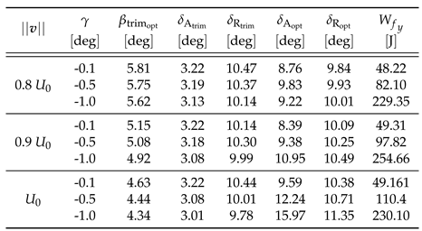
Table 2 summarizes the conditions and the obtained results of the optimal landing including the sideslip angle at trim within the optimization variables. Now, the third column refers to the sideslip angle at trim found by the optimization algorithm, whereas the fourth and the fifth columns refer to the trim control settings and associated with .
Comparing Table 1 and Table 2, one can immediately notice that, in all cases, landing with some misalignment with respect to the runway leads to significantly lower tire wear. For example, in the case with and , the value of the work of the friction forces results equal to for fixed sideslip and to for optimized sideslip, with a reduction of about .
Moreover, looking at the initial conditions, it is possible to verify that the difference between the optimized sideslip angle and the fixed one is limited, i.e. about , which is reflected in slightly different trim control settings in terms of both aileron and rudder deflections.
To understand where this difference might be originated, the work dissipation time histories for both cases are plotted in Figure 6, which shows the contribution to the work of the friction forces, i.e. the function to-be-integrated in Eq. (27), as a function of time, for both approaches, i.e. without optimizing the sideslip at trim () and including this variable within the optimization parameters (). The bottom figure shows the overall tire wear displaying the function to-be-integrated in Eq. (27). Additionally, in the top figures, the separated contributions of the left and right main gear are reported: each subplot details the trend of the lateral force (first row), the lateral velocity (second row), and the resulting contribution to the work of the friction forces (third row).
As already mentioned, the work dissipation exhibits a highly irregular behavior, with peaks and discontinuities due to the complex ground-tire interaction, and the contribution given by three landing gear legs, which touch the runway at different instants. Hence, finding a physical interpretation of the obtained results is complex. Nonetheless, some useful considerations can be made.
Preliminary, given the landing and wind conditions considered in this example, it is important to notice that, being the roll angle at trim positive (), the aircraft touches the ground with the right leg first at second 2.8, followed by the left one at second 3.5, and, finally, by nose one. The detailed plot of the contact between the nose gear and the terrain is not shown in Figure 6 as it occurs at second 6.5 circa and does not significantly affect the overall tire wear.
We may now consider the top plots of Figure 6, which allow comparing the cost function contributions of the left and right main gears for the two cases. As a first observation, notice that the airplane initially undergoes a lateral displacement to the right (positive ) when only the right leg is in contact with the ground (between seconds 2.8 and 3.5). Then, after the second leg touches the ground (after second 3.5), a lateral overshoot to the left is experienced by the system (negative ). This trend is common to both landing approaches. Focusing on the first seconds of the touchdown (between seconds 2.8 and 3.5), it is evident that the peak of the tire wear for the right gear (top-right plot, third subplot) is clearly higher if the airplane heading is misaligned with respect to the runway, . However, when also the second leg gets in contact with the terrain (after second 3.5), the combined effect of the airplane motion and the initial misalignment with respect to the runway leads to a lower lateral overshoot and lower friction forces. As a result, the overall tire wear, which corresponds to the integral of the curves displayed at the bottom plot, is lower if a mild misalignment of the airplane with respect to the runway () is considered immediately before the airplane touches the ground. This justifies the difference in the performance obtained for the two landing approaches studied in this work and reported in Table 1 and Table 2. Similar considerations, not shown here for the sake of brevity, can be derived from other tests considered in this work.
6. Conclusions
This work deals with the optimization of the landing technique in crosswind conditions for minimum tire wear.
In order to achieve this goal, first, a simulator capable of handling the landing maneuver in crosswind conditions was developed. The simulator considers a three-dimensional model of the coupled airplane-landing gear system.
The airplane is modeled as a rigid body in a three-dimensional domain, subject to gravitational, propulsive, aerodynamic, and reaction forces and moments. The aerodynamics, linearized about a suitable condition and rendered through the classical stability and control derivatives, considers also the presence of a generic steady wind. Along with the nonlinear model of the system, a process for trimming the airplane during flight considering the wind was developed. The output of the trim in windy conditions can be used as initial conditions for the landing simulation.
The landing gear, instead, is a simplified anterior tricycle with each leg composed of a tire, modeled as a linear spring with a parallel damper, and a nonlinear oleo-pneumatic shock absorber. A contact detection algorithm was also implemented to find when and which leg has touched the ground or rebounded. Once the contact between one or more legs and the ground is detected the reaction forces are included in the simulation. Such reaction forces are modeled according to the usual simplified friction models. From the computation of the reaction forces and the motion of the aircraft on the ground, using the simple Achard theory, it was also possible to estimate the tire wear for each tire during landing.
The landing simulator model was tested with an airplane model inspired by the Lockheed Jetstar.
Next, the optimization of the tire wear during landing in crosswind conditions was performed. To do so, the simulation code was embedded inside an optimization algorithm with the aim of determining an optimal landing technique in terms of the sideslip angle before touchdown and control deflection after touchdown.
From the results obtained in this work and from extensive practice, the following conclusions can be derived.
- The landing simulator model is able to handle and combine airborne and ground landing phases considering generic wind conditions. The simulation, being based on a nonlinear three-dimensional model of airplane dynamics, is also compliant with the physics of the landing maneuver and considers the asymmetric contact among the wheels and the terrain, that is typically involved during crosswind conditions.
- A simulation parametric study shows that touchdowns at lower approach speeds and lower vertical speeds are associated with lower tire wear. This fact, which is however expected, is due to lower lateral forces, generated during the contact between legs and ground, that lead to reduced wear.
- From the parametric analysis, it was also possible to show that in crosswind landing specific control settings after touchdown may reduce wear: the minimum wear is obtained if, after touchdown, ailerons are deflected towards the upwind direction, whereas the rudder is set near the trim conditions, maintaining a crossed controls setting.
- A three-variable optimization problem aimed at finding the sideslip angle at trim and the lateral-directional controls after touchdown associated with the minimum tire wear can be also formulated. It was demonstrated that a mild track misalignment, due to a difference between airplane heading and runway direction is associated with reduced tire wear. In fact, even if this misalignment produces higher wear during the first instants after the first wheel touches the ground, the combination of the lateral forces on all legs, the motion of the aircraft once landed and the initial airplane misalignment generates lower wear over the landing.
Clearly such promising but still preliminary results need further analysis before they could be considered consolidated. In terms of extension of the optimization of tire wear, in fact, it could be interesting to consider different airplanes with different dimensions and weights. Moreover, since the analysis of this paper has focused on lateral friction, and, hence, on the wear due to lateral wheel drift, a complete study including wheel spin-up, longitudinal friction, and brakes should be performed.
Finally, as far as the landing simulator is concerned, possible improvements may include the development of a control system capable of handling the whole landing maneuver from descent to airplane stop, and the enrichment of the aircraft aerodynamic modeling, possibly including different flap settings.
Author Contributions
S.C. and C.E.D.R. developed the original formulation and composed the present paper. L.C. contributed to the refinement of the formulation, carried out the quantitative analyses, and contributed to the writing of the present paper. All authors participated equally in the development of the body of the work, with discussions and critical comments on the results. All authors have read and agreed to the published version of the manuscript.
Funding
This research received no external funding.
Institutional Review Board Statement
Not applicable.
Informed Consent Statement
Not applicable.
Data Availability Statement
All the data and the numerical tools used in this work may be obtained by contacting the corresponding authors.
Conflicts of Interest
The authors declare no conflict of interest.
Appendix A. Reference aircraft data inspired by Lockheed Jetstar
The reference airplane data used in this work are reported in Table A1–Table A4. The main sources from which data were gathered are:
- scaled drawings (used when more accurate geometric data were unavailable);
- supplier catalogues, [30].
Whenever real aircraft data were unavailable, aircraft preliminary design methods were applied in order to retrieve the missing information.
Unless otherwise specified, data are referred to power approach configuration, which includes light gross weight, landing gear extended, 40% flaps, and sea level conditions.

Table A1.
Lockheed Jetstar geometric and inertial properties
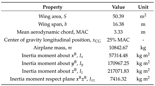
Table A2.
Lockheed Jetstar aerodynamic properties
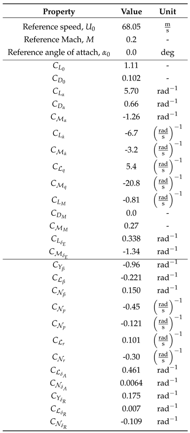
Table A3.
Lockheed Jetstar main landing gear properties
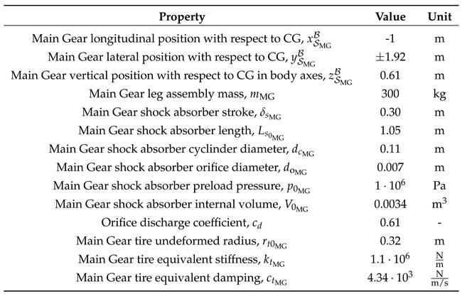
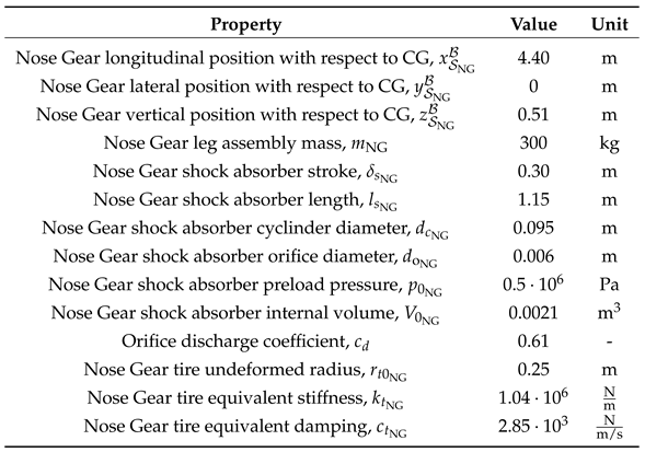
Table A4.
Lockheed Jetstar nose landing gear properties
References
- Aibus S.A.S.. A Statistical Analysis of Commercial Aviation Accidents, 1958 - 2021. Technical report, Airbus, 2021.
- Riboldi, C.E.D.; Cacciola, S.; Ceffa, L. Studying and Optimizing the Take-Off Performance of Three-Surface Aircraft. Aerospace 2022, 9. [CrossRef]
- Bottasso, C.L.; Croce, A.; Leonello, D.; Riviello, L. Optimization of Critical Trajectories for Rotorcraft Vehicles. Journal of the American Helicopter Society 2005, 50, 165–177. [CrossRef]
- Trainelli, L.; Gennaretti, M.; Bernardini, G.; Rolando, A.; Riboldi, C.E.D.; Redaelli, M.; Riviello, L.; Scandroglio, A. Innovative helicopter in-flight noise monitoring systems enabled by rotor-state measurements. Noise Mapping 2016, 3, 190–215. [CrossRef]
- Riboldi, C.E.D.; Rolando, A. Layout Analysis and Optimization of Airships with Thrust-Based Stability Augmentation. Aerospace 2022, 9, 393. [CrossRef]
- Dreier, M.E. Introduction to Helicopter and Tiltrotor Simulation; AIAA (American Institute of Aeronautics and Astronautics), 2007.
- Evans, P.E. Modeling and simulation of tricycle landing gear at normal and abnormal conditions. Master’s thesis, West Virginia University, 2010.
- Wang, C.; Holzapfel, F. Modeling of the Aircraft Landing Behavior for Runway Excursion and Abnormal Runway Contact Analysis. 2018 AIAA Modeling and Simulation Technologies Conference, 2018. [CrossRef]
- Daniels, J.N. A method for landing gear modeling and simulation with experimental validation. Technical report, NASA Contractor Report 201601, 1996.
- Yang, X.; Yang, J.; Zhang, Z.; Ma, J.; Sun, Y.; Liu, H. A review of civil aircraft arresting system for runway overruns. Progress in Aerospace Sciences 2018, 102, 99–121. [CrossRef]
- Barnes, A.; Yager, T. Enhancement of Ground Handling Simulation Capability. Technical report, Advisory Group for Aerospace Research and Developement, 1998.
- Vechtel, D. How future aircraft can benefit from a steerable main landing gear for crosswind operations. CEAS Aeronautical Journal 2019, 11, 417–429. [CrossRef]
- Vechtel, D.; Meissner, U.; Hahn, K. On the use of a steerable main landing gear for crosswind landing assistance. CEAS Aeronautical Journal 2014, pp. 293–303.
- Shepherd, A.; Catt, T.; Cowlind, D. The simulation of aircraft landing gear dynamics. Proceeding of 18th Congress of the International Council of the Aeronautical Sciences 1992.
- Evans, P.; Perhinschi, M.; Mullins, S. Modeling and Simulation of a Tricycle Landing Gear at Normal and Abnormal Conditions. AIAA Modeling and Simulation Technologies Conference, 2018. [CrossRef]
- Lei, Z.; Hongzhou, J.; Hongren, L. Object-oriented landing gear model in a PC-based flight simulator. Simulation Modelling Practice and Theory 2008, 16, 1514–1532. [CrossRef]
- Wen, Z.; Zhi, Z.; Qidan, Z.; Shiyue, X. Dynamics Model of Carrier-based Aircraft Landing Gears Landed on Dynamic Deck. Chinese Journal of Aeronautics - CHIN J AERONAUT 2009, 22, 371–379. [CrossRef]
- Alroqi, A.; Wang, W. Comparison of Aircraft Tire Wear with Initial Wheel Rotational Speed. International Journal of Aviation, Aeronautics, and Aerospace 2015, 2.
- Reye, K. Zur Theorie der Zapfenreibung [On the theory of pivot friction]. Civilingenieur 1860.
- Archard, J.F. Contact and Rubbing of Flat Surfaces. Journal of Applied Physics 1953, 24, 981–988. [CrossRef]
- Sethuramiah, A.; Kumar, R. Modeling of Chemical Wear: Relevance to Practice; Elsevier, 2015; pp. 1–232.
- Cacciola, S.; Riboldi, C.E.D.; Arnoldi, M. Three-surface model with redundant longitudinal control: Modeling, trim optimization and control in a preliminary design perspective. Aerospace 2021, 8, 139. [CrossRef]
- Riboldi, C.E.D.; Rolando, A. Thrust-Based Stabilization and Guidance for Airships without Thrust-Vectoring. Noise Mapping 2023, 10, 344. [CrossRef]
- Clark, D.; Kroll, J. General Purpose Airborne Simulator - Conceptual Design Report. Technical report, NASA Flight Research Center, 1966.
- Heffley, R.; Jewell, W. Aircraft Handling Qualities Data. Technical report, NASA Flight Research Center, 1972.
- Smith, H. Flight-Determined Stability and Control Derivatives for and Executive Jet Transport. Technical report, NASA Flight Research Center, 1975.
- Roskam, J. Airplane Design; Number pt. 4 in Airplane Design, DARcorporation, 1985.
- Torenbeek, E. Synthesis of Subsonic Airplane Design; Delft University Press: Delft, 1982.
- Currey, N. Aircraft Landing Gear Design: Principles and Practices; AIAA Education Series, American Institute of Aeronautics & Astronautics, 1988.
- The Goodyear Tire & Rubber Company. Goodyear aviation data book, 2021.
- De Marco, A.; Duke, E.; Berndt, J. A General Solution to the Aircraft Trim Problem. AIAA Modeling and Simulation Technologies Conference and Exhibit, 2007. [CrossRef]
- Muskardin, T. Autonomous landing of fixed-wing aircraft on mobile platforms. PhD thesis, Universidad de Sevilla, Departamento de Ingeniería de Sistemas y Automática, 2020.
- Popov, V.L.; Heß, M.; Willert, E. Handbook of Contact Mechanics; Springer Berlin, Heidelberg, 2019.
- van der Veen, J. An analytical approach to dynamic irregular tyre wear. Master’s thesis, Eindhoven University of Technology, Department Mechanical Engineering, 2007.
- Alroqi, A.; Wang, W. Reduction of Aircraft Tyre Wear by Pre-Rotating Wheel Using ANSYS Mechanical Transient. Advanced Engineering Forum 2016, 17, 89–100. [CrossRef]
- MATLAB. Optimization Toolbox User’s Guide; The MathWorks Inc.: Natick, Massachusetts, 2022.
- Nelson, R. Flight Stability and Automatic Control; Aerospace series, McGraw-Hill, 1989.
- Sadraey, M.H. Aircraft design: A systems engineering approach; Aerospace Series, John Wiley and Sons: Chichester, 2012.
Figure 1.
Airplane and landing gear reference frames.
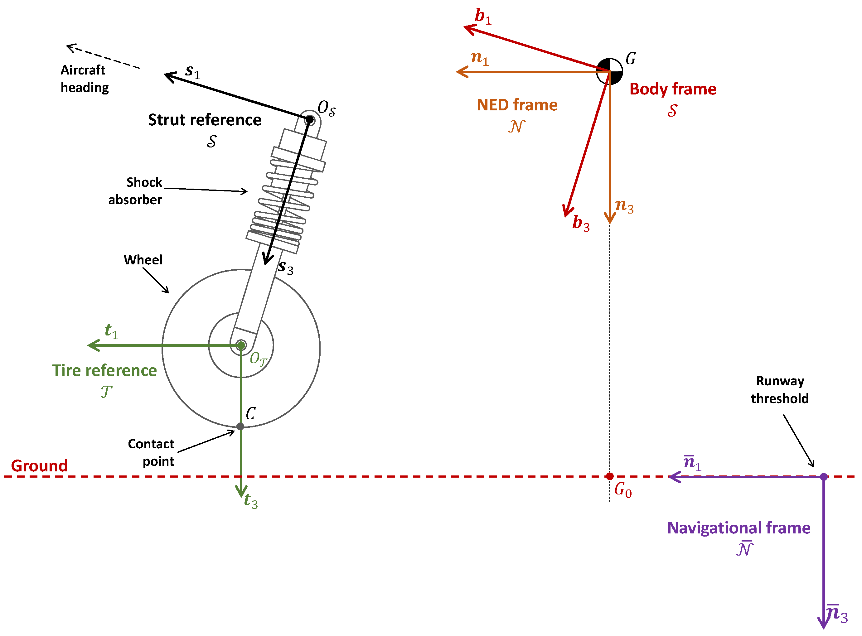
Figure 2.
Point-contact tire model.
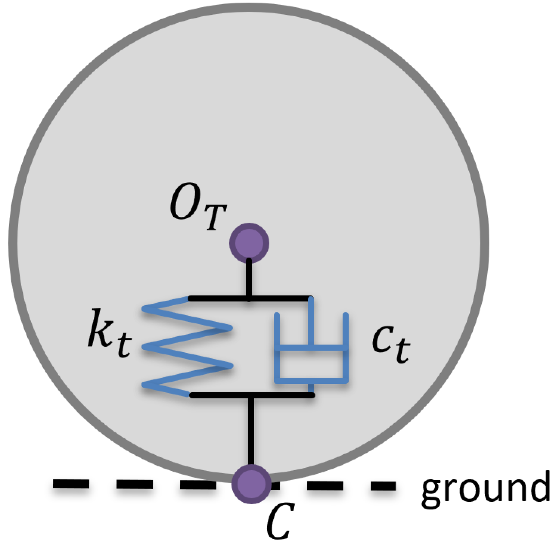
Figure 3.
Sideslipped (wings-low) crosswind approach (adapted from [32]).
Figure 3.
Sideslipped (wings-low) crosswind approach (adapted from [32]).
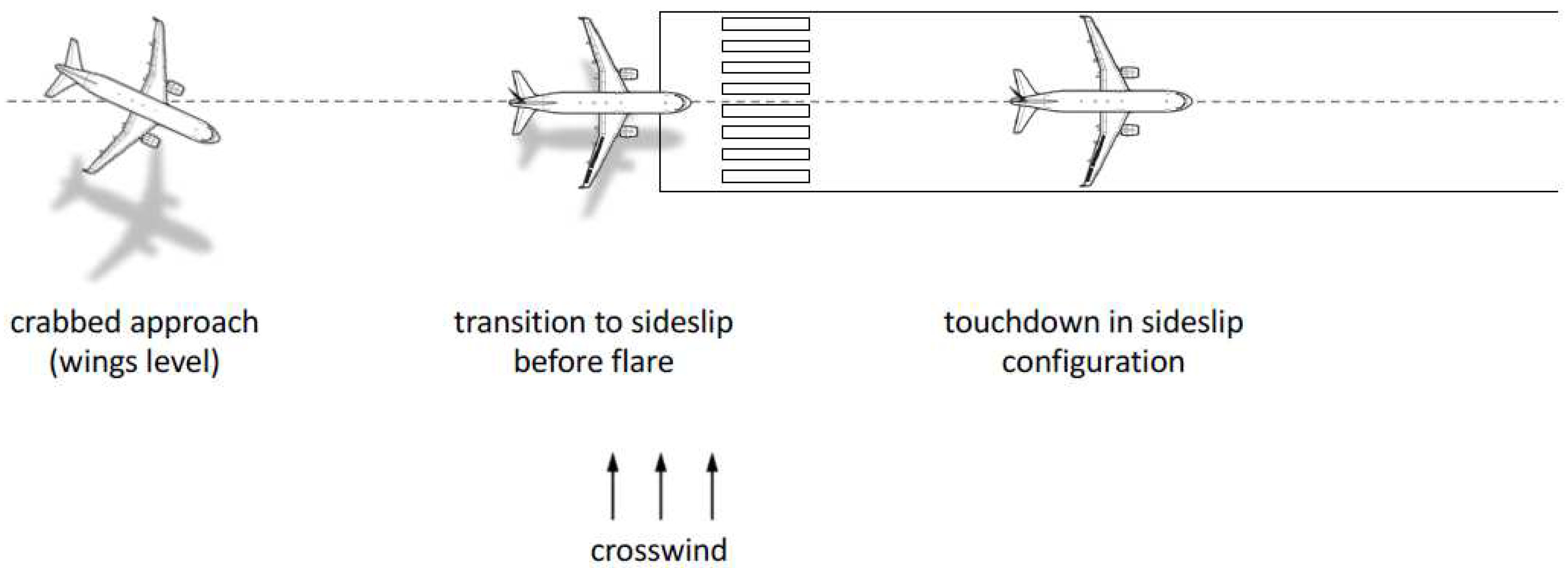
Figure 4.
Example of crosswind landing - = -0.1o, TAS = 54.44 , Wind direction/wind speed: .
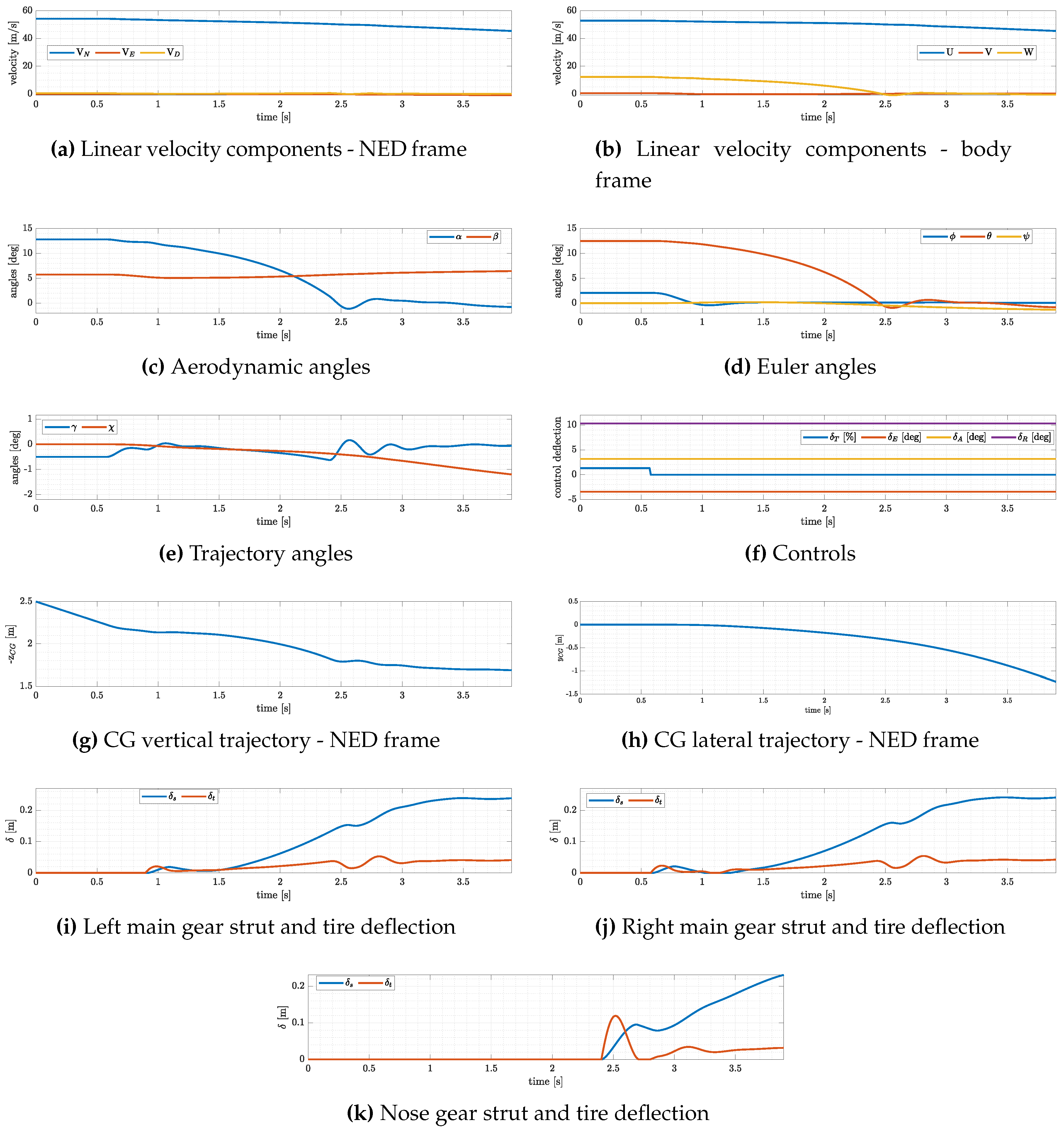
Figure 5.
Cost function mapping. Left plot: null crosswind; right plot: crosswind .
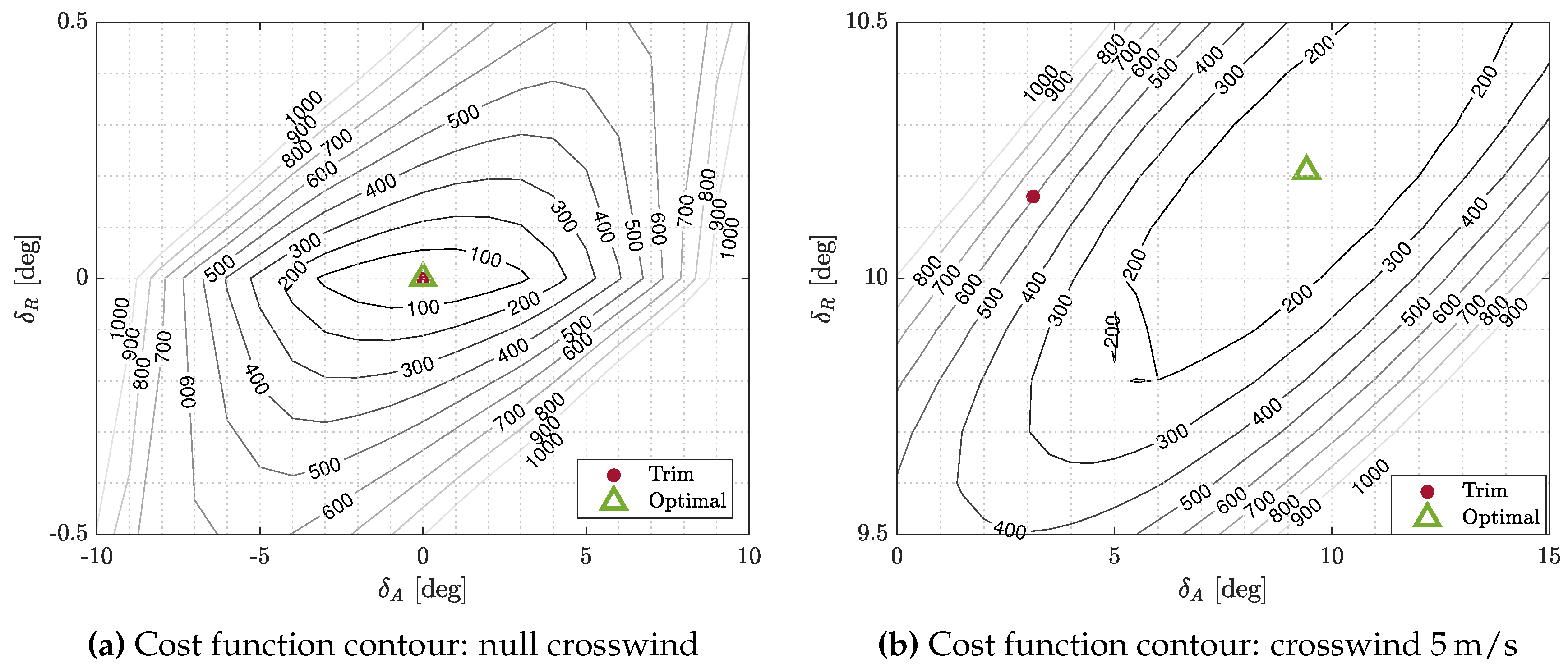
Figure 6.
Comparison between two optimal landing approaches at and . Blu dashed line (): optimization without sideslip at trim as in Table 1; red solid line (): optimization including sideslip at trim within the optimization variable as in Table 2. Top-left: contribution of the left main gear; top-right plot: contribution of the right main gear; bottom plot: overall tire wear.
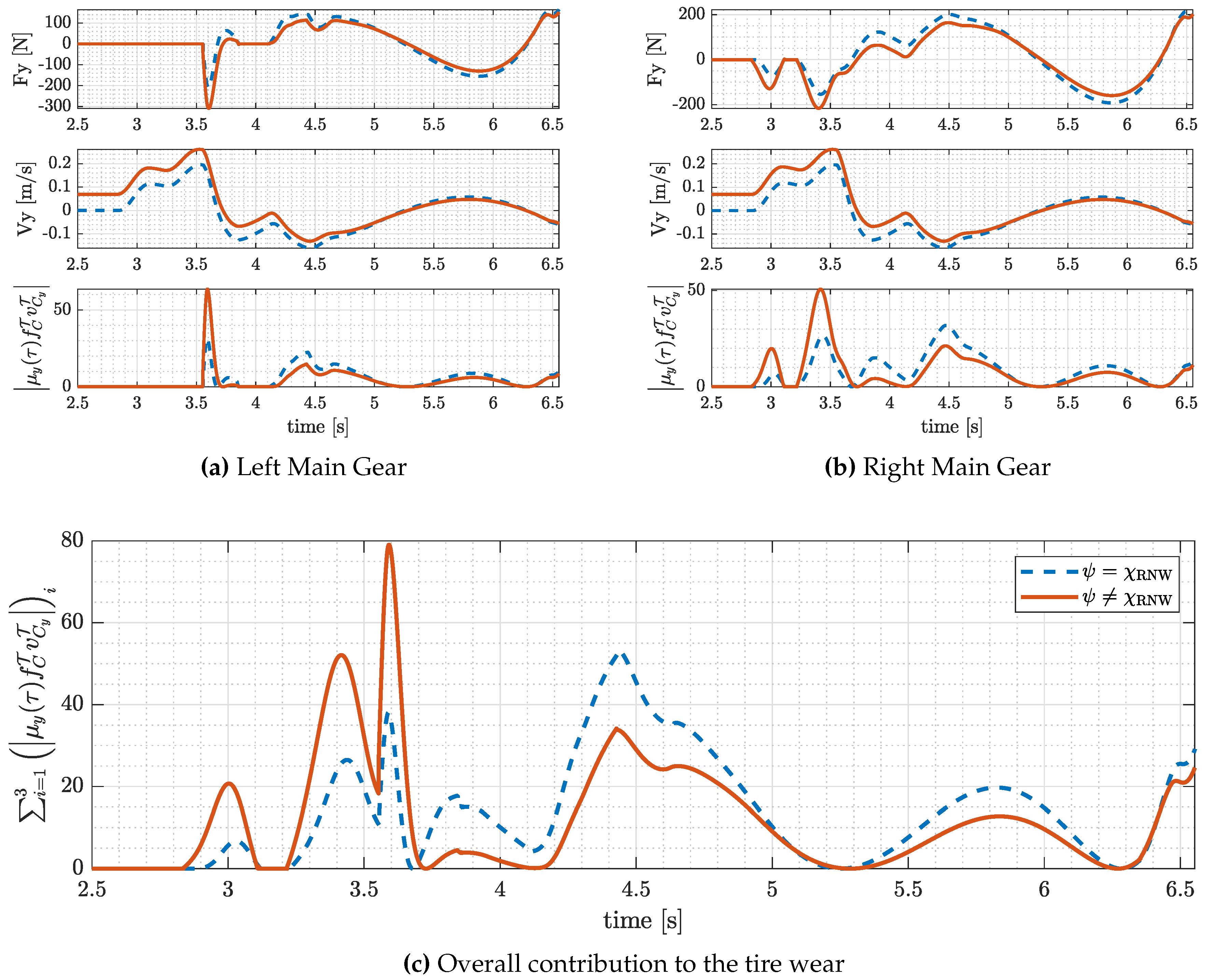
Table 1.
Optimization test conditions and results. Lateral wind speed . Variable as defined in Appendix A.
Table 1.
Optimization test conditions and results. Lateral wind speed . Variable as defined in Appendix A.
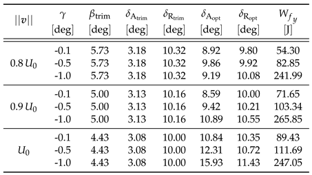
Table 2.
Optimization test conditions and results including sideslip angle within the optimization variables. Lateral wind speed . Variable as defined in Appendix A.
Table 2.
Optimization test conditions and results including sideslip angle within the optimization variables. Lateral wind speed . Variable as defined in Appendix A.
Disclaimer/Publisher’s Note: The statements, opinions and data contained in all publications are solely those of the individual author(s) and contributor(s) and not of MDPI and/or the editor(s). MDPI and/or the editor(s) disclaim responsibility for any injury to people or property resulting from any ideas, methods, instructions or products referred to in the content. |
© 2023 by the authors. Licensee MDPI, Basel, Switzerland. This article is an open access article distributed under the terms and conditions of the Creative Commons Attribution (CC BY) license (http://creativecommons.org/licenses/by/4.0/).
Copyright: This open access article is published under a Creative Commons CC BY 4.0 license, which permit the free download, distribution, and reuse, provided that the author and preprint are cited in any reuse.


