
Submitted:
26 April 2023
Posted:
27 April 2023
You are already at the latest version
Abstract
The use of logistic regression models in data analysis and machine learning has expanded in recent years and has become the primary preference of researchers in risk assessment studies across a wide range of scientific fields. From the assessment of credit risk in financial institutions to the estimation of risk factors for traffic accidents or the identification of etiological factors for chronic diseases. All logistic models are natural extensions of the simple binary model, and their interpretation is based on it. Using the data of a cross-sectional study on the risk factors of traffic collisions, the two main extended models of logistic techniques, multinomial and ordinal logistic regression, are presented in the article in detail. Emphasis is placed on the use of ordinal regression since the outcome variable of the collision data is defined as ordinal measurement reflecting a latent continuous scale.
Keywords:
vehicle crash data
; collision risk
; ordinal logistic regression
; multinomial logistic regression
; proportional odds model (POM)
; partial proportional odds model (PPOM)
1. Introduction
Often in empirical research it is necessary to estimate the risk of escalating outcomes defined through an ordinal variable. The binary logistic regression model is adequate for the case of a binomial event but is not suitable for the estimation of a multinomial outcome with internal ordering [1,2,3,4]. Usually, the analysis of this type of data i.e., a response variable with multiple outcomes and a set of predictor variables, is performed through the multinomial logistic regression model. The latter arises as an extension of the simple logistic model and its functional definition is an expansion of the properties of binary logistic regression [5,6,7].
It is known that when the response variable of a model is binary the equation (logit) of logistic regression that applies to the odds of success is
where x1, x2,…,xk are the values of a set of independent variables Χ1,Χ2,...,Χk.
In the case where the response variable is categorical with m > 2 categories, there are m-1 non-redundant logits that can be defined. One of the categories of the dependent variable is defined as the reference category (baseline category = j) and based on it, m-1 different logits are estimated with general form
or equivalent
For each of the previous logit there is a set of coefficients derived for the k independent variables of the multinomial model. Each one estimates the odds of occurrence of category i regarding the reference category j. For example, if the model's response variable has three levels, then two sets of non-zero coefficients will result comparing two categories (levels) of the variable with regard to the reference category. For the reference category, the coefficients of the corresponding logit are all zero. We can estimate all possible logits of a multinomial logistic model, by changing the reference category. Multinomial logistic regression is nearly equivalent to running a series of binary logistic regressions on the data. The main difference is that the equations are fit simultaneously rather than separately, which imposes an additional constraint, the predicted probabilities of all possible outcomes must sum to 1 [6].
The multinomial logistic regression model can be modified and be simpler when the outcome is ordinal. In this case, the ordering of the response variable is useful to be incorporated into the analysis to simplify the interpretation and to increase the power of the multinomial model. Ordinal logistic regression is a special type of multinomial regression, which can be valuable when the response variable is ordinal [6,8,9,10,11,12].
Starting again from the simple logistic regression model, having the occurrence of a binary event as the dependent variable,
we will modify it to accommodate the case where the event of interest is not a discrete single outcome (e.g., yes/no) but a set of possible outcomes, coded according to the values of an ordinal variable. Specifically, in an example of vehicle data, the event could be the number of car crashes coded as 0=no crash, 1=up to two crashes, 2=three or more. In this case, for each of the possible values of the crashes’ variable Y, we have the following odds:
For the last category of the crashes’ variable, the odds (for y ≤ 2) is equal to unity.
The prior odds (1) and (2) can be restated overall as:
or equivalent
In the general case, where the dependent variable in the model is ordered with m>2 categories, there are m-1 non-redundant logits that can be estimated linearly. In the simple case of a univariate model, with one independent variable X, the equation used is slightly modified
The previous model has a negative slope to bring its interpretation into line with the usual interpretation of the coefficients of linear models [13]. In linear models, the response variable is related to the predictors through a positive covariation formula. That is, the equation of the model, as long as the coefficients are positive, defines the response variable as covarying in the same direction as the predictor variables. In ordinal regression, if there are positive coefficients in the model, the increase in the values of a predictor variable corresponds to an increased odds of the event of interest, which is defined by Y values less than or equal to a certain value (events achieved for y ≤ j). If, therefore, we have a positive slope in the model, this would mean that the resulting logits would associate increasing values of X with decreasing values of Y. In order to have the known covariation form, as in the other linear models, so that we can infer how much the log-odds of having lower values of Y will change when X increases, we use a negative sign.
We could have a positive slope in the ordinal model, if the equation defining the logits had the form
In this case, the positive slope refers to Y values that correspond to odds for y > j. That is, a unit increase in the variable X estimates the increase of the log-odds of the complementary events of y ≤ j. Some software uses the equation with a positive sign. In such cases, the exponential transformation of b corresponds to the odds of y > j. We can reverse the exp (b) to calculate the probability of y ≤ j. [13,14].
The logits of the ordinal model are estimated by m-1 linear equations, which differ from each other only in the constant term αj. The coefficients of the independent variables are the same. This practically means that, the effect of each independent variable is the same across all logits (across all levels of the response variable). The latter is an assumption that must be checked when using ordinal regression. Because of its necessity, the ordinal regression model is also called Proportional Odds Model (POM). The constant term of each logit is called threshold and is not of particular interest when interpreting the results. It has the same interpretation as the constant term in linear regression. The coefficients of the independent variables, which are the same for all logits are referred to as location. When using the ordinal model, the assumption of the proportional odds needs to be tested inferentially as well as graphically.
The ordinal regression coefficients are estimated through the maximum likelihood method, as in the other logistic models. The method estimates the regression coefficients and tests them inferentially by means of Wald's statistic. In addition, the coefficients and the overall fit of the model can be evaluated through the likelihood ratio test. In order to interpret the coefficients in terms of odds, they must be transformed exponentially. Some software, such as SPSS calculates the regression coefficients without their exponential transformation. The user must therefore calculate for each variable Χk, the quantity and the corresponding confidence intervals. According to the model definition, each coefficient estimates the change in cumulative odds for the value j of Y (all events i ≤ j), for each unit increase of the independent variable Xk. The coefficients of the independent categorical variables are interpreted in a similar way. For each category c of an independent categorical variable Xk, the quantity defines the cumulative odds ratio (CumOR) of category c regarding the reference category.
The ordinal logistic model has greater power than the multinomial one by providing a single estimation of the odds for an ordinal variable without multiple comparisons of the individual logits [6,15,16]. We will use it against multinomial logistic regression with the help of field data concerning the effect of sleepiness, fatigue and sleep disorders on car crashes [17].
2. Materials and Methods
The study involved 1,366 drivers who were asked about incidents of falling asleep and fatigue while driving in the year of the field survey. They were also asked about possible sleep disturbances and the frequency of daytime sleepiness (Epworth scale) [18]. Study data were collected through door-to-door visits using a team of field interviewers that received appropriate training. An easy-to-use self-administered questionnaire was distributed and informed consent was requested by all subjects prior to participation. Participants were asked to complete the questionnaire at the time of the visit, while the interviewers’ role was limited to the supply of advice and possible clarifications. Anonymity was ensured by coding all personal data and confidentiality was safeguarded by restricting access to personal data to a limited authorized number of researchers. Drivers’ socio-demographic variables regarding gender, age, educational level, etc. as well as characteristics concerning the driving experience (e.g. years of driving license possession, distance driven since driving license acquisition) were included in the questionnaire. The number of crashes caused by the participants since driving license acquisition was measured using an open- ended question.
The variables of falling asleep and fatigue were defined by the following scales:
(a) Number of fall-asleep incidents while driving during the previous 12 months. They were assessed through the rate of involvement in three different situations such as near miss, fall asleep incidents and found off the road due to falling asleep. The rate of involvement was measured through a six-point scale ranging from 0 = never to 5 = very often.
(b) Fatigue while driving in the last 12 months, was measured through the rate of occurrence of 9 different risky driving situations such as, not remembering the last few kilometers, having incoherent thoughts while driving, having difficulties in keeping the head up, missing road signs, etc. The rate of occurrence was measured using a six-point scale (0 = never, 1 = 1–2 times, 2 = 3–4 times, 3 = 5–6 times, 4 = 7–8 times and 5 = 9+ times).
(c) Daytime sleepiness in the last 12 months, was examined through the 8-point Epworth scale. Some situations of Daytime Sleepiness were classified as, dozing or falling asleep (i) while sitting and reading, (ii) while watching TV, and (iii) while sitting inactive in a public place. The participants were requested to rate their chances, on a scale of 0 = never to 5 = 9+ times, of dozing or falling asleep in each of these situations in the year prior to the research. The total scale score ranged from 0-40. Higher total scores revealed greater tendency towards Daytime Sleepiness.
(d) Symptoms of sleep disorders in the last month, were measured through seven items referring to the quality of sleep. In particular, participants were asked to report the rate of dealing with seven different sleeping problems such as ‘‘Thinking while squirming in bed for long”, ‘‘Woke up in the middle of the night or early in the morning”, ‘‘Felt tired when waking up in the morning”. A four-point scale (0 = never, 1 = 1 time per week, 2 = 2–3 times per week, and 3 = 4+ times per week) was used to measure the symptoms of sleep disorder.
The scales (b) to (d) were summed up according to increased report of fatigue episodes while driving, the total score of sleepiness and the items of sleep disorders. The number of fall-asleep incidents while driving, because of its highly skewed distribution, was recoded to binary, with values, 1=at least one incident of falling asleep in the last 12 months and 2=no incident of falling asleep.
Data analysis
Data analysis was initially performed using an ordinal regression model with the number of crashes as dependent variable. The independent variables of the analysis were drivers' sex, years of license possession, drivers' age, alcohol consumption in glasses per week, number of fall-asleep incidents (as a binary variable, yes/no) and the three cumulative scales of fatigue while driving, daytime sleepiness and sleep disorders. The number of driver-attributable crashes was defined through an ordinal variable with values: 0 = no crashes, 1 = up to two crashes, 2 = three crashes or more. In order to evaluate and compare the results of the ordinal model with those of multinomial logistic regression, the study data was reanalyzed using a multinomial model with the same set of variables. All statistical analyses were performed using SPSS v.28 statistical software (IBM SPSS, Armonk, NY, USA).
3. Results
Initially, the sleep variables were displayed graphically in terms of their effect on the number of crashes, through cumulative frequencies plots. For instance, the fall-asleep (while driving) incidents variable, was presented through the cumulative plot of Figure 1. The shape of the plot shows that, at low crash rates the cumulative frequency of drivers with no incidents of falling asleep is consistently higher than those who had at least one incident. This difference in the cumulative frequencies gradually decreases, until the complete convergence of the two lines in 100% of the observations. Because drivers with incidents of falling asleep while driving report lower rates in the low crash categories and higher rates in the higher categories, we expect the regression coefficient of the falling asleep variable in the model to be positive. Similar illustrations emerge if we construct the cumulative frequencies plots of the fatigue, sleep disorders and daytime sleepiness variables. These three scale variables, in order to be represented graphically, were recoded as binary with categories values lower or higher than their median. Plots of the fatigue and sleep disorders are shown in Figure 2 and Figure 3.
Cumulative frequency plots are essential before proceeding with the analysis, at least for the variables of primary interest. It is the introductory criteria for using ordinal logistic regression, ensuring, at a descriptive level, the proportional odds assumption. The shape that should appear in the plots is similar to that shown in Figure 1, with no intersection of the two lines except at their final convergence in 100% of the observations. Apart from this descriptive procedure, it is necessary to inferentially test the parallel lines assumption (each line corresponds to a logit of the analysis) [19].
Table 1 evaluates the logistic ordinal model using the likelihood ratio statistic. The dependent variable of the model is the number of crashes while the predictor variables are drivers' sex, years of license possession, drivers' age, alcohol consumption in glasses per week, sleepiness while driving, fatigue while driving, frequency of daytime sleepiness and sleep disorders. Based on the sampling distribution of the ratio, the probability that all model coefficients are equal to 0 is p < 0.001. Table 1 also evaluates the multinomial model. The hypothesis of all coefficients being equal to 0 also rejected.
Table 2 illustrates the assessment of the proportional odds assumption through the test of parallel lines. The null hypothesis of equal slopes (location) for all logits is not rejected (p=0.363). In case the assumption of parallel lines was not satisfied, the multinomial logistic regression or other ordinal model could be used as an alternative.
Table 3 shows the coefficients of the two logits of the analysis, which differ only in terms of the values of the threshold. The regression coefficients (location) are the same in both estimates. The estimation of the coefficients of the two logits at a single value, resulted from the parallel line test. From the model’s parameters, it appears that the sleep variables had a significant effect on causing collisions. Specifically, incidents of fatigue and sleep while driving had a positive effect on increasing the likelihood of crashes while short daytime naps had a negative (protective) effect. From the exponential transformation of the model parameters, it resulted that drivers with incidents of sleepiness while driving had an approximately 73% higher risk of having at least one crash (1 or more) than drivers without incidents of sleepiness (Cum OR=1.73, 95% CI: 1.32 – 2.28, p < 0.001). Furthermore, each unit increase in the driving fatigue scale increased the odds of at least one crash by approximately 7% (Cum OR=1.07, 95% CI: 1.04 – 1.09, p < 0.001). In the opposite direction, each unit increase in the daytime sleepiness scale decreased the odds of crashes by 1-0.96 = 4% (Cum OR=0.96, 95% CI: 0.94 – 0.98, p < 0.001).
The odds obtained from the previous exponential transformations are similar to those from a multinomial logistic model. However, in ordinal regression the estimates concern the logits of the model as a whole, because the ordinal model makes the assumption that the slopes (location) are the same in all the logits of the analysis (parallel lines assumption). In order to establish the appropriateness and completeness of the ordinal model against the multinomial, in case of ordinal response variables, we reanalyzed the data with the help of a multinomial logistic model.
Table 4 presents the parameters of the multinomial logistic model for each of the analysis logit. The first part of the table refers to the logit of at most two crashes (1-2 crashes) versus none. The corresponding odds ratios were related to the years of holding a license (the risk increases as the years of driving increase) and to the values of the sleep variables. Increased frequency of fatigue incidents increased the odds of collision by approximately 5% for each unit of the fatigue cumulative scale (OR=1.05, 95% CI: 1.02-1.09, p < 0.001). The dichotomous variable defining the presence of a fall-asleep incident while driving was also related to the risk of collisions. Drivers with at least one episode of falling asleep in the last 12 months had a 77% higher odds ratio for a crash than other drivers (OR = 1.77, 95% CI: 1.29-2.45, p < 0.001). The variable of sleep disorders was also significant to the risk of collision. For each unit increase in the scale of sleep disorders, the odds of collision increased by 4% (OR=1.04, 95% CI: 1.01-1.07, p=0.019). Finally, the increased frequency of sleep incidents during the day, i.e., short-duration sleeps such as a momentary rest or nap, reduces the odds ratio of crashes by approximately 5% for every 1-point increase in the daytime sleepiness scale (OR=0.95, 95% CI: 0.93 – 0.98, p < 0.001).
The second part of the table shows the regression coefficients and the corresponding odds ratios for the logit of a higher number of crashes (≥ 3 crashes) versus none. At this point, the main variables that increased the risk of collisions were, mainly, episodes of fatigue and sleepiness while driving in the last 12 months. For each unit increase in the scale of fatigue, the odds ratio of collisions increased by 11% (OR =1.11, 95%CI: 1.06-1.15, p < 0.001). Also, drivers who had at least one episode of drowsy driving in the last year were twice as likely to crash compared to those who reported no episode (OR=2.08, 95% CI: 1.33-3.26, p < 0.001). In this second logit, sleep disorders did not seem to affect the risk of collisions, while daily, short-duration sleep seemed to be protective in the event of greater number of crashes (OR=0.97, 95% CI: 0.93-0.99, p = 0.035).
4. Discussion
Ordinal logistic regression, if the proportional odds assumption holds, estimates the cumulative odds for ordinal outcomes without assessment of the individual logits. In the example presented, the odds for the variable of collisions were estimated with a single value for each predictor variable of the ordinal model. Numerically, each regression coefficient estimates the average change in the log-odds for increasing level of collisions. And this for each unit increase of a predictor variable, as long as the other variables remain constant.
Furthermore, compared to the multiple logits estimated by multinomial regression, the coefficients of ordinal model summarize the change in collision risk in a manner that is both concise and uniform. For example, the average change along all levels of crashes, for 1-point increase in fatigue scale is, according to the ordinal model, about 7%. That is, about as much as the average change in the odds of the two logits estimated by multinomial regression: 5% for the logit of 1-2 crashes vs none and 11% for the logit of 3 and more. The same applies to the coefficients of the other predictor variables of the two models except for the variable of sleep disorders. For the scale of sleep disorders in the multinomial model, significant differences were found in the logit of 1-2 crashes (p=0.019) but not for the logit of 3 or more (p=0.712). In the ordinal model, which summarizes the average change along all levels of the collision’s variable, no significant differences emerged (p=0.138).
Ordinal and multinomial regression, in our example, yielded similar results including similar predicted probabilities for the number of collisions. Both models are reasonable choices for the case of an ordinal dependent variable. The advantage of using ordinal regression over multinomial is that it increases the power of the analysis since it incorporates the ordering of the dependent variable in the model. In this way, the estimation of a single slop/odds ratio is achieved for all categories of the ordinal variable instead of the estimation of multiple logits for smaller subsets of the data [6]. The disadvantage is that ordinal logistic regression estimates an average effect of the predictor variables across all outcome levels—so if the effects are in fact different, the model will miss this. The estimation of an average effect requires the fulfillment of the proportional odds assumption. Otherwise, the use of the ordinal model may lead to incorrect results.
Multinomial logistic model is an alternative to ordinal regression when the proportional odds assumption does not apply. However, its use requires the estimation of a larger number of parameters compared to the ordinal one, so the number of degrees of freedom used in the model-fitting process can make excessive demands on the dataset. Moreover, the interpretation of its results is clearly more complex and non-concise than that of ordinal regression [15].
An additional disadvantage of multinomial regression is that it does not take into account the ordinal nature of the response variable, and therefore its statistical power to detect associations with the explanatory variables is suboptimal, especially when these associations are linear in either a positive or negative direction [15]. In an extreme case, an explanatory variable may be linearly associated with the ordinal outcome, with small monotonic changes in odds across all outcome levels. It is possible in such a case, the individual logits of the multinomial model do not detect significant differences in odds while the overall cumulative odds of the explanatory variable being significant. Unlike multinomial regression, ordinal regression is applied to response variables with ordinal effect, since it works with the cumulative distribution for the response variable, and the parameter it fits for each association represents the general trend across the ordinal values of the response variable.
In cases of data where the response variable is ordinal and the proportional odds assumption does not apply for all predictor variables, either multinomial regression or the partial proportional odds model (PPOM) can be used [20,21,22,23]. The PPOM can model some of the predictor variables with the proportional odds assumption (provided that this is hold for them) while for the rest can introduce special parameters in the logistic equation that vary for the different compared categories. For example, if the explanatory variables Χi and Χj satisfy the proportional odds assumption, then b’s for Χi and Χj (bi and bj) are the same for all levels of the response variable. On the other hand, if the variable Χz does not meet the proportional odds assumption, then b for Χz (bzj) are free to differ for different levels (j) of the response variable [24]. The interpretation of PPOM coefficients is similar to the interpretations of multinomial and proportional odds regression coefficients.
The partial proportional odds model is a generalized case of ordinal regression and can be run in SAS software through the LOGISTIC procedure and in STATA through the GOLOGIT2 module. SPSS does not have a related procedure.
5. Conclusions
The extensive use of logistic models in data analysis requires their application in a well-argued manner depending on the measurement level of the response variable and the assumptions that must hold. The binary logistic regression is the basis of all these models, however without being able to cover the cases of response variables with multiple categories or, even more, the cases of variables with ordered categories. In these latter cases, such as the example of car crashes presented previously, it is recommended to use the ordinal logistic model, provided the proportional odds assumption holds. Otherwise, the use of multinomial or partial proportional odds regression is suggested. Partial proportional odds model is an extension of the POM in order to handle the predictor variables for which the proportionality of odds does not apply. In these models, variables that meet the assumption of proportional odds are treated with the logic of ordinal regression, while those for which it does not apply are analyzed with the logic of multinomial regression.
Author Contributions
Conceptualization-Original Draft Preparation, C.G. and J.C; Supervision, C.G.; Writing-Review and Editing, V.N., M.P., and G.T. All authors have read and agreed to the published version of the manuscript.
Funding
This study received no external funding.
Data Availability Statement
Data are available upon request.
Conflicts of Interest
The authors declare no conflict of interest.
References
- Hosmer DW, Lemeshow S, Sturdivant RX. Applied Logistic Regression. 3nd Edition John Wiley and Sons, New York 2013.
- Collett D. Modelling Binary Data. Chapman and Hall, London 1991.
- Joseph MH. Logistic Regression Models. 1st Edition Chapman and Hall/CRC, New York 2009.
- Agresti A. Categorical Data Analysis. 3rd Edition, John Wiley and Sons, Hoboken, New Jersey 2013.
- Kwak C, Clayton-Mathews A. Multinomial logistic regression. Nursing Research 2002, 51(6), 404-10. [CrossRef]
- Sainani KL. Multinomial and ordinal logistic regression. PM&R 2021, 13, 1050-1055. [CrossRef]
- Park KH, Kerr PM. Determinants of Academic Performance: A Multinomial Logit Approach. The Journal of Economic Education, 1990, 21, 101-111. [CrossRef]
- Anderson JA. Regression and Ordered Categorical Variables. Journal of the Royal Statistical Society 1984, 46, 1-30. [CrossRef]
- Anderson JA, Philips PR. Regression, Discrimination and Measurement Models for Ordered Categorical Variables. Applied Statistics 1981, 30, 22-31. [CrossRef]
- Campbell KM, Donner A. Classification Efficiency of Multinomial Logistic Regression Relative to Ordinal Logistic Regression. Journal of the American Statistical Association 1989, 84, 587-591. [CrossRef]
- Bender R, Grouven U. Ordinal logistic regression in medical research. Journal of the Royal College of Physicians of London 1997, 31, 546-551.
- French B, Shotwell MS. Regression Models for Ordinal Outcomes. JAMA 2022, 328, 772-773. [CrossRef]
- Norusis M. Advanced Statistical Procedures Companion. Prentice Hall, Upper Saddle River, NJ 2008.
- Flom P. Multinomial and ordinal logistic regression using PROC LOGISTIC. Conference: Northeast SAS Users Group, 2010.
- Warner P. Ordinal logistic regression. J Fam Plann Reprod Health Care 2008, 34, 169-170. [CrossRef]
- Koletsi D, Pandis N. Ordinal logistic regression. Am J Orthod Dentofacial Orthop 2018, 153, 157-158. [CrossRef]
- Gnardellis C, Tzamalouka G, Papadakaki M, Chliaoutakis JE. An investigation of the effect of sleepiness, drowsy driving, and lifestyle on vehicle crashes. Transportation Research Part F Traffic Psychology and Behaviour 2008, 11, 270-281. [CrossRef]
- Johns MW. A new method for measuring daytime sleepiness: the Epworth sleepiness scale. Sleep. 1991,14, 540–545. [CrossRef]
- Brant R. Assessing Proportionality in the Proportional Odds Model for Ordinal Logistic Regression. Biometrics, 1990, 46, 1171-1178. [CrossRef]
- Peterson B, Harrell FE. Partial Proportional Odds Models for Ordinal Response Variables. Journal of the Royal Statistical Society 1990, 39, 205-217. [CrossRef]
- Singh V, Dwivedi SN, Deo SVS. Ordinal logistic regression model describing factors associated with extent of nodal involvement in oral cancer patients and its prospective validation. BMC Medical Research Methodology, 2020, 20:95. [CrossRef]
- Abreu MN, Siqueira AL, Cardoso CS, Caiaffa WT. Ordinal logistic regression models: application in quality of life studies. Cad Saude Publica, 2008, 24 Suppl. 4, s581-591. [CrossRef]
- Mooradian J, Ivan JN, Ravishanker N, Hu S. Analysis of driver and passenger crash injury severity using partial proportional odds models. Accident Analysis & Prevention, 2013, 58: 53-58. [CrossRef]
- Sasidharana L, Menéndez M. Partial proportional odds model-An alternate choice for analyzing pedestrian crash injury severities. Accident Analysis & Prevention, 2014, 72, 330-340. [CrossRef]
Figure 1.
Plot of fall-asleep variable.
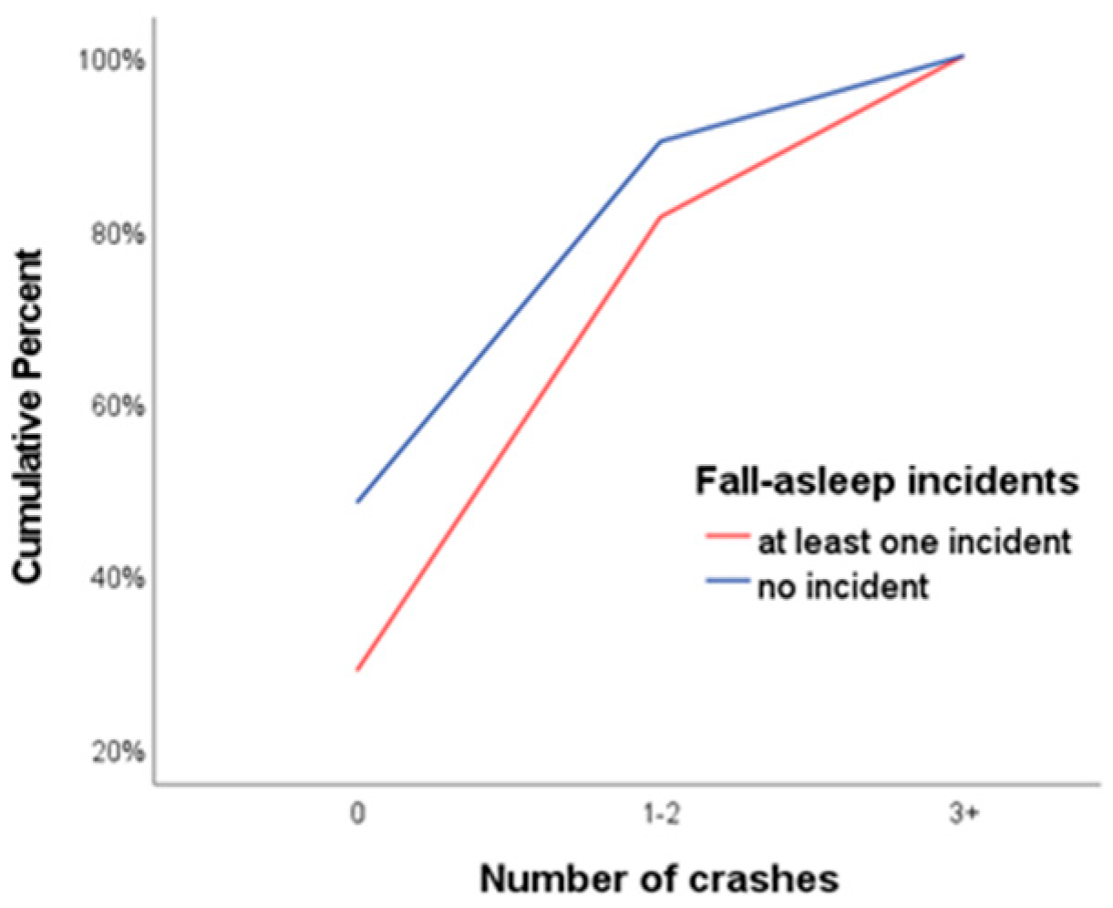
Figure 2.
Plot of fatigue variable.
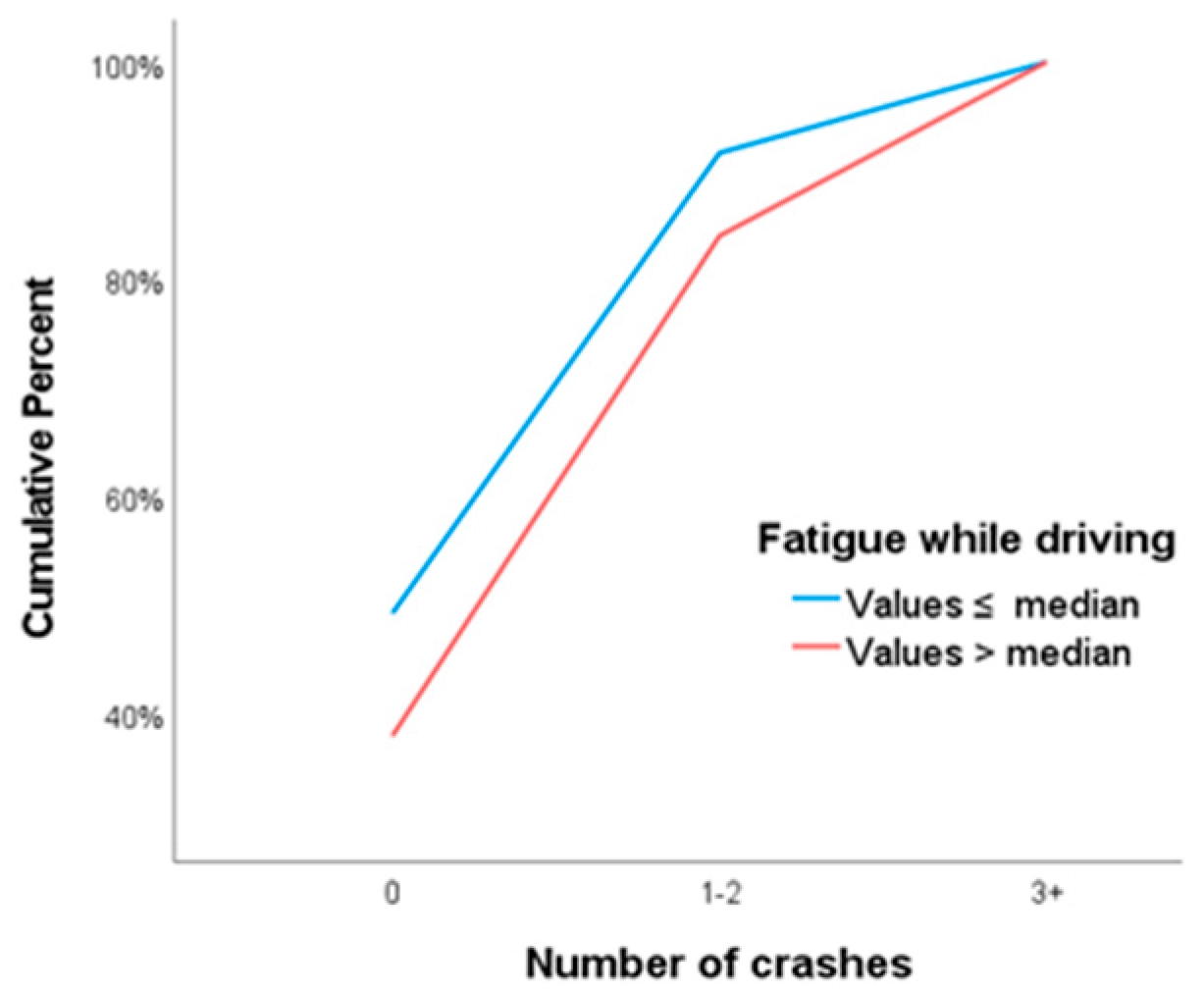
Figure 3.
Plot of sleep disorders.
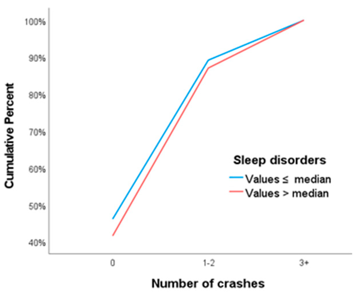

Table 1.
Ordinal and multinomial model fitting with the number of crashes as response variable.
| Model Fitting Information | ||||
| Model | -2LL | Chi-Square | df | p value |
| Ordinal Intercept Only Final model |
2615.6 2508.5 |
107.9 |
8 |
<0.001 |
| Multinomial Intercept Only Final model |
2615.6 2500.6 |
115.1 |
16 |
<0.001 |
Table 2.
Parallel lines test for the ordinal model.
| Test of Parallel lines | ||||
| -2LL | Chi-Square | df | p value | |
| Null Hypothesis General |
2508.5 2499.8 |
8.8 |
8 |
0.363 |
Table 3.
Cumulative odds ratios derived from the ordinal logistic regression with the number of crashes as response variable.
Table 3.
Cumulative odds ratios derived from the ordinal logistic regression with the number of crashes as response variable.
| Ordinal logistic model | ||||
| B | Cum OR | 95%CI | p value | |
| Threshold Crashes=0 |
0.219 |
1.24 |
0.74 - 2.09 |
0.409 |
| Crashes=1-2 | 2.608 | 13.57 | 7.88 -23.36 | <0.001 |
| Location | ||||
| Age | -0.006 | 0.99 | 0.97 -1.01 | 0.494 |
| Sex (Men vs Women) | -0.006 | 0.99 | 0.79 -1.25 | 0.958 |
| Years of license | 0.035 | 1.04 | 0.97 -1.61 | 0.004 |
| Alcohol consumption glasses/week | 0.011 | 1.01 | 0.99 -1.03 | 0.141 |
| Fatigue scale | 0.065 | 1.07 | 1.04 -1.09 | <0.001 |
| Day sleepiness | -0.038 | 0.96 | 0.94 -0.98 | <0.001 |
| Sleep disorders | 0.021 | 1.02 | 0.99 -1.05 | 0.138 |
| Fall-asleep incidents (yes vs no) | 0.548 | 1.73 | 1.32- 2.28 | <0.001 |
Table 4.
Odds ratios derived from the multinomial logistic regression with the number of crashes as response variable (0 crashes = reference category).
Table 4.
Odds ratios derived from the multinomial logistic regression with the number of crashes as response variable (0 crashes = reference category).
| Multinomial logistic model | ||||
| Number of crashes | B | OR | 95%CI | p value |
| 1-2 crashes | ||||
| Age | -0.011 | 0.99 | 0.97 -1.01 | 0.305 |
| Sex (Men vs Women) | -0.002 | 0.99 | 0.77 -1.29 | 0.988 |
| Years of license | 0.030 | 1.03 | 1.00 -1.06 | 0.025 |
| Alcohol consumption glasses/week | 0.011 | 1.01 | 0.99 -1.03 | 0.241 |
| Fatigue scale | 0.052 | 1.05 | 1.02 -1.09 | <0.001 |
| Day sleepiness | -0.048 | 0.95 | 0.93 -0.98 | <0.001 |
| Sleep disorders | 0.038 | 1.04 | 1.01 -1.07 | 0.019 |
| Fall-asleep incidents (yes vs no) | 0.573 | 1.77 | 1.29- 2.45 | <0.001 |
| 3+ crashes | ||||
| Age | -0.006 | 0.99 | 0.96 -1.03 | 0.729 |
| Sex (Men vs Women) | -0.031 | 0.97 | 0.64 -1.47 | 0.882 |
| Years of license | 0.051 | 1.05 | 1.01 -1.10 | 0.014 |
| Alcohol consumption glasses/week | 0.021 | 1.02 | 0.99 -1.05 | 0.081 |
| Fatigue scale | 0.100 | 1.11 | 1.06 -1.15 | <0.001 |
| Day sleepiness | -0.036 | 0.97 | 0.93 -0.99 | 0.035 |
| Sleep disorders | 0.009 | 1.01 | 0.96 -1.06 | 0.712 |
| Fall-asleep incidents (yes vs no) | 0.733 | 2.08 | 1.33- 3.26 | <0.001 |
Disclaimer/Publisher’s Note: The statements, opinions and data contained in all publications are solely those of the individual author(s) and contributor(s) and not of MDPI and/or the editor(s). MDPI and/or the editor(s) disclaim responsibility for any injury to people or property resulting from any ideas, methods, instructions or products referred to in the content. |
© 2023 by the authors. Licensee MDPI, Basel, Switzerland. This article is an open access article distributed under the terms and conditions of the Creative Commons Attribution (CC BY) license (http://creativecommons.org/licenses/by/4.0/).
Copyright: This open access article is published under a Creative Commons CC BY 4.0 license, which permit the free download, distribution, and reuse, provided that the author and preprint are cited in any reuse.


