
Submitted:
23 April 2023
Posted:
24 April 2023
You are already at the latest version
Abstract
Magnetic nanoparticles (MNPs) have attracted a great interest in nanomedical research. MNPs exhibit many important properties, particularly, magnetic hyperthermia for selective killing of cancer cells is one of them. In hyperthermia treatment, MNPs act as nano-heaters when they are under the influence of an alternating magnetic field (AMF). In this work, micromagnetic simulations have been used to investigate the magnetization dynamics of a single-domain nanoparticle of magnetite in an external AMF. Special attention is paid to the circumstances dealing with a dynamic phase transition (DPT). Besides, we focus on the influence of the orientation of the magnetic easy-axis of the MNP on the dynamic magnetic properties. For amplitudes of the external AMF above certain critical value, the system is not able to follow the magnetic field and it is found in a dynamically ordered phase; whereas for larger amplitudes, the state corresponds to a dynamically disordered phase and the magnetization follows the external AMF. Our results suggest that the way how the order-disorder DPT takes place, and both the metastable lifetime as well as the specific loss power (SLP), are strongly dependent on the interplay between the orientation of the magnetic easy-axis and the amplitude of the external AMF.
Keywords:
dynamic phase transition
; alternating magnetic field
; magnetic nanoparticle
; hyperthermia
; specific loss power
1. Introduction
It is well-established that nanoparticles with sizes ranging between 1 and 100 nm, exhibit different and appealing characteristics compared with their micro and macro counterparts. In recent years, magnetic nanoparticles (MNPs) have been used in areas of nanotechnology, in particular for biomedical applications [1,2] where precise delivery of anticancer drugs and selective killing of cancer cells is desirable. Magnetic hyperthermia treatment [3] is based on the use of nanoparticles dispersed in a magnetic fluid. When MNPs are under the presence of an external AMF, they are able to heat a specific area of the body causing cells death in tumor tissue [6]. During such process, two relaxation mechanisms for MNPs are known, namely, the Néel [4] and Brown [5] modes. In the former, magnetic moments rotate inside the nanoparticle due to the action of the external AMF. In contrast, in Brown relaxation, magnetic moments are locked to the magnetic easy-axis of the MNP and the AMF causes a mechanical rotation of the particle as a whole. The heat released to the medium is either caused by the friction between the surface of MNPs and the surrounding magnetic-fluid, or by the power dissipated through the hysteresis losses [7]. The heating efficiency of a MNP under an external AMF is expressed in the physical quantity called specific loss power (SLP) [8,9].
The dynamic response of a MNP in an external time-dependent magnetic field of amplitude and period P, is not instantaneous and it exhibits a delay in time. Time delay of the magnetization gives rise to the appearance of two possible regimes [10,11,12]: a dynamically ordered phase (DOP) and a dynamically disordered one (DDP), which depend on the relationship between P, and the metastable lifetime [13,14]. In the DOP (see Figure 1a), magnetization is not able to follow the magnetic field, giving rise to a high value of the average magnetization. In DDP (see Figure 1b), magnetization follows the magnetic field even though with a dependent delay, and it gets to be reversed resulting in a well-defined hysteresis loop. In this case, the metastable lifetime, which is the elapsed time to go from the saturation state and pass through zero magnetization, can be computed.
The universal aspects that allow a dynamic phase transition have been studied in some works [10,11,12,13,14]. B. K. Chakrabarti and M. Acharyya [12] showed that magnetic response in time by an external field depends on the competing time scales, i.e. the time period of oscillation of the external perturbation and the typical relaxation time. When the time period of oscillation is comparable with the effective relaxation time, symmetric hysteresis loops around the origin are obtained. A breaking of the symmetry of the hysteresis appears when the driving frequency of the field increases. This phase transition depends on the field amplitude and temperature. On the other hand, G. Korniss et. al. [11] studied through Monte Carlo simulations the two-dimensional kinetic Ising model with a square-wave oscillating external field of period P. Their results showed that the system undergoes a dynamic phase transition when the half-period of the field is comparable to the metastable lifetime , which in turn depends on temperature T and the field amplitude . Several metastable states were also studied by P. A. Rikvold et. al. [14] for an impurity-free kinetic Ising model with nearest neighbor interactions and local dynamics under a magnetic field, in the framework of droplet theory and Monte Carlo simulation. They demonstrated that metastable lifetimes exhibited magnetic field and system-size dependences. Additionally, W. D. Baez and T. Datta [13], established for a two-dimensional ferromagnetic kinetic Ising model with oscillating field and next-nearest neighbor interactions, that metastable lifetimes are determined by the lattice size, amplitude and frequency of the external field, temperature and additional interactions present in the system.
Micromagnetic models [15], based on the solution of the Landau-Lifshitz-Gilbert equation [16,17,18], have also allowed a theoretical description of micro and nanoscale magnetization processes above the exchange length. Micromagnetism integrates classical and quantum mechanical effects, where the spin operators of the Heisenberg model are replaced by classical vectors and also accounts for exchange interaction. The main assumptions of the model are: the distribution of the magnetic moments is considered discrete throughout the volume of the magnetic system by means a set of discretization cells and at the same time it is approximated by a density vector , which is continuous and differentiable with respect to both space and time t, and it can be written in terms of a unit vector field where is the saturation value of constant norm.
Despite all the studies devoted to systems exhibiting dynamic phase transitions, little effort has been paid to the role played by the spatial orientation of the easy-axis of a single nanoparticle relative to the direction and sense of the external applied oscillatory field. It must be stressed that different orientations of the magnetic easy-axis must be interpreted as different ensamble microstates occurring during Brown rotation, so by fixing the magnetic easy-axis in each microstate considered, we can drive our attention to the Néel relaxation at each Brown rotation step. Thus, the purpose of the present work is to calculate the metastable lifetimes for different amplitudes and orientations of the magnetic easy-axis as well as the interplay between these two parameters. To do so, micromagnetic simulations were performed using the Ubermag [19] package based on the Object Oriented Micromagnetic Framework (OOMF) [20].
The remainder of the paper is organized as follows. In Section 2 we present an overview of the micromagnetic background of a MNP with a given easy-axis of magnetization, its geometrical and physical aspects and computational details. Numerical results are presented in Section 3 where a proposal of dynamic phase diagram is presented, and in Section 4 we make a summary and a brief conclusion of the main results.
2. Theoretical model and Computational details
2.1. Micromagnetic energy
According to the micromagnetic theory, the energy density is composed by a series of contributions according to the properties of the magnetic material. In our micromagnetic system, consisting of a single-domain magnetic nanoparticle of magnetite, contributions to the energy density are exchange, demagnetization, Zeeman and magnetocrystalline anisotropy [21]:
where A is the stiffness constant accounting for an effective ferromagnetic interaction, is the demagnetizing field caused by magnetostatic interaction, JAm is the permeability of free space, is the magnetic field, K is the anisotropy constant and denotes the magnetic easy-axis unitary direction. In this work, the magnetic field is a sinusoidal wave applied along the -direction of the form with , amplitude , frequency f and initial displacement . The competition between the different micromagnetic energy contributions on minimization, determines the equilibrium distribution of magnetization [22]. At each point or discretization cell of the magnetic sample, an effective field is calculated by means of:
with
being the energy of the system over the entire volume V of the sample.
2.2. Landau– Lifshitz–Gilbert (LLG) equation
The time evolution of the magnetization of a magnetic nanoparticle, with radius R and saturation magnetization , is ruled by the Landau-Lifshitz equation with Gilbert damping, which reads as follows [16,17,18],
where denotes the dimensionless damping parameter and mAs is the gyromagnetic ratio. LLG equation is strictly valid only at absolute zero temperature and the normalized magnetization vector is . The system transfers energy and angular momentum from the movement of the magnetic moments to other degrees of freedom through the parameter[23]. The first term of LLG equation is associated with the gyromagnetic ratio that promotes a uniform precession of the magnetization around the effective field. The second term is a phenomenological damping parameter that accounts for the energy loss of the system before reaching the equilibrium state.
2.3. Metastable lifetime and Specific Loss Power (SLP)
Ferromagnetic systems attached to a periodically oscillating magnetic field can exhibit order-disorder DPT. A significant aspect in DPT is the metastable lifetime. To study this DPT behavior, first the system must be fully magnetized with all the magnetic moments aligned along the direction of the maximum external magnetic field. Once the field is allowed to change in time, we analyze the conditions under which the magnetization becomes reversed and it passes through the zero value of magnetization. The elapsed time between these two magnetic states corresponds to the metastable lifetime and it is schematically shown in Figure 2. This is a measure of the time it takes for the system to escape from the metastable saturation state in the free-energy landscape.
A complete decay of the metastable phase occurs only in a dynamically disordered phase, as shown in Figure 1b. In this phase, the metastable lifetime is comparable with the period of the external magnetic field, the magnetization follows the magnetic field and its average over one period is close to zero. Consequently, the hysteresis loop is symmetric. The area enclosed by the hysteresis loop is the irreversible work dissipated in form of heat, which is quantified by the SLP energy. This heat is given by the following relationship [24,25]:
where is is the mass density of the particle. The integration is done over one period of the oscillating magnetic field. The thermal energy quantified by SLP is an important magnitude for magnetic hyperthermia studies[3]. SLP depends on several parameters, such as and f of the external field, composition and system size, shape and magnetic state of the MNP [8].
2.4. Computational model
The simulation and the dynamic response of the magnetization of our micromagnetic system is carried out by means of the Ubermag micromagnetic software package [19,20]. The discrete representation of the magnetization distribution is obtained through the finite-difference method as is schematically represented in Figure 3a, where we have considered a magnetic nanoparticle with pseudo-spherical geometry and a crystal structure corresponding to magnetite . The physical properties used in our simulation for magnetite are shown in Table 1.
A discretization cubic cell of 2 nm edge was employed. This linear dimension is much smaller than the exchange length () as required, which in the case of magnetite is given in Table 1. A typical value of for a bulk ferrimagnetic material like magnetite was employed [28]. The frequency of the AMF was MHz, which is within the range of the radio-frequency currently used in magnetic hyperthermia [29]. Additionally, the initial displacement considered was .
In this work, initially the system is prepared in a fully positively magnetized state along the -direction and different orientations of the magnetic easy-axis of anisotropy are considered. In Cartesian coordinates, we have , where the azimuthal angle was fixed at , and the different values of the polar angle were ranged between and .
3. Results and Discussion
The magnetization in the micromagnetic model is calculated by solving the LLG equation at zero temperature. First, we calculate the component of magnetization for amplitudes of mT and mT, as is shown in Figure 4a–c and Figure 4c–e respectively. Simulations were performed for , and . First, note that for an amplitude of the external AMF of mT, and for each orientation of the easy-axis, the system is found in a DOP. In contrast, a DDP is evidenced for mT. Hence, the results shown in Figure 4 demonstrate that both DOP and DDP depend on the of AMF and the easy-axis orientation. A sharp reversal of magnetization takes place for values small, i.e. .
Now that it is known the dependence of DOP and DDP with the amplitude of the external AMF, we can calculate the critical amplitudes for which the DPT of the type DOP-DDP occurs for a wide range of values of the polar angle as shown in Figure 5. To achieve this dynamic magnetic phase diagram, it was necessary to carry out systematically several simulations like those shown in Figure 4, in order to determine the critical amplitudes of the AMF for which the magnetization was not able to be switched. As can be observed in this figure, the lower region corresponds to the DOP whereas the upper region indicates the DDP. Thus, the DPT is strongly dependent on both the amplitude and the easy-axis orientation of the particle, and both quantities follow a non-linear relationship. Moreover, as the easy-axis is oriented nearly-parallel to the magnetic field direction, DPT takes place at higher values of amplitude. In contrast, for an orientation nearly-perpendicular of DPT occurs at lower amplitude values. Thus, a nearly perpendicular orientation of makes the magnetic system less rigid, giving rise to a DPT at small magnetic fields. This fact constitutes a way of tuning the magnetically hard or soft character of the system.
As larger amplitudes of the external AMF are considered, the magnetization quickly escapes from its metastable state and slowly decreases as is oriented nearly-perpendicular to the external AMF direction. In contrast, the small the amplitude, more time is required to escape from the metastable state, and quickly decreases with the increase of . Thus, we conclude that the metastable lifetime not only depends on the amplitude of the external AMF at a given frequency, but also on the easy-axis orientation. Several numerical results for different orientations of were obtained as is shown in Figure 6.
In addition, we also obtained the dynamic hysteresis loops for different easy-axis orientations of at a given field amplitude. The respective results are shown in Figure 7 for mT. Hence, as already unveiled, it is clear that the angle of the easy-axis strongly affects magnetization reversal. As long as the easy-axis is oriented nearly perpendicular to the external AMF main direction, coercivity is significantly reduced. This presumably implies that as the external field is applied in a direction away from that of the easy-axis, it is easier to "pull" the magnetization out of the easy direction of anisotropy through different paths in phase space. This fact is also the responsible for the crossing of branches observed in the descending and ascending branches of the hysteresis loops at the switching fields, which is more noticeable for large values of . This peculiar and surprisingly behavior of the crossing of hysteresis branches has been already demonstrated to occur in similar systems [30,31]. The crossing of the ascending and descending branches of the magnetization is observable when the applied external AMF is considerably far of the easy-axis, and this fact is associated with the energy minimum around the metastable state. Mathews et al. in [30] demonstrated that such scenario can be occur for a Stoner–Wohlfarth particle with a unique anisotropy. Hence, we have been able to show that the crossing of branches is significantly affected by the orientation of the particle.
On the other hand, the micromagnetic energy contributions for each orientation of the easy-axis are shown in Figure 8. Figure 8a–c show the exchange energy for , and , respectively. Figure 8d–f stand for the demagnetization energy, Figure 9a–c for the anisotropy energy and Figure 9d–f for Zeeman energy, and for the same angles. We observe that the main micromagnetic energy contribution is given by the Zeeman energy, whereas the exchange energy contribution is the smallest one.
For the case of , a zoom of the anisotropy and Zeeman energies is shown for clarity in Figure 9. Some jumps at , and are observed for both the ascending and descending field branches, which is consistent with a sort of transition zone. In particular, a significant increase in the value of the anisotropy energy is observed for , which implies that the magnetic moments are not aligned with the easy-axis of the MNP. At the same value of , a minimum in the Zeeman energy is observed, which implies an alignment of the magnetic moments with the field direction. In contrast, for , the opposite scenario takes place. This means, that during the transition zone, magnetic moments become magnetically frustrated, as a consequence of the competition between these two energies.
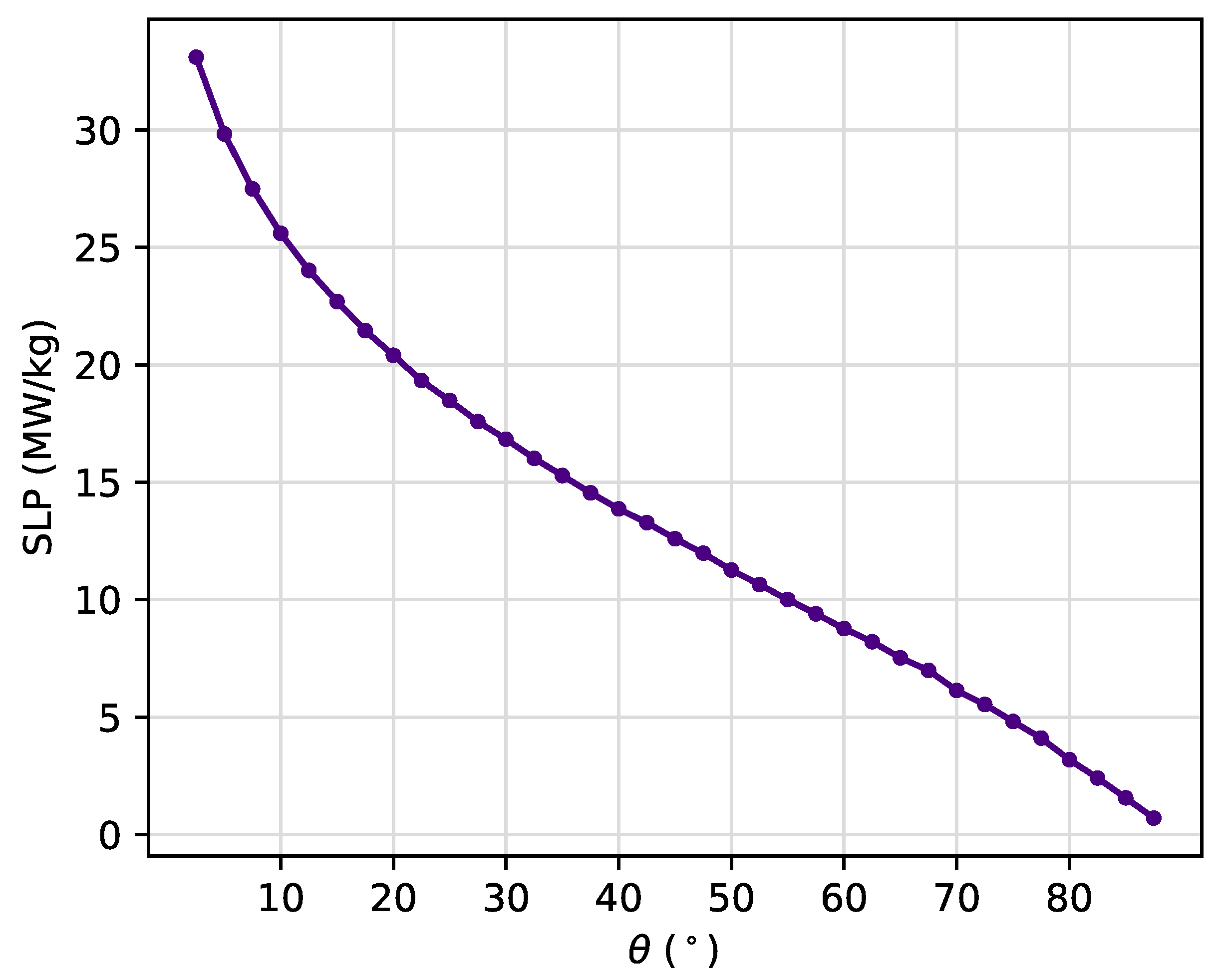
Finally, all of the above results lead to ask about the amount of heat that can be dissipated in terms of the specific loss power, which is proportional to the hysteresis loop area. Such quantity was computed using Equation 5, and the respective angular dependence is shown in Figure 10. The SLP is maximized when the easy-axis of the MNP is oriented nearly parallel to the magnetic field direction, that is, for small angle values there is a greater efficiency in the amount of heat released to the environment. This is a novel result, because in the literature it is known that the specific loss power depends on parameters such as the size of the particles, the frequency and amplitude of the external AMF [8,9], but to the best of our knowledge, no studies on this specific regard have been addressed up to now. This result may shed lights on new ways to maximize the SLP for hyperthermia purposes.
4. Conclusions
In this study, we have presented numerical calculations of the micromagnetic properties and dynamic critical behavior of the magnetization for a single-domain MNP of magnetite under the influence of an oscillating magnetic field. Exchange, demagnetization, anisotropy and Zeeman energies were considered and the time evolution of the magnetization was obtained by solving the LLG equation at zero temperature. The numerical simulation was performed by means of the micromagnetic simulator Ubermag package based on the Object Oriented Micromagnetic Framework (OOMMF). We studied the effect of the orientation of the easy-axis of the MNP upon the critical values of the amplitude of the external AMF dealing with a dynamic phase transition. Thus, results were summarized in a proposal of a dynamic magnetic phase diagram. In addition, we calculated the time it takes for the magnetization to achieve the first-passage through the zero magnetization value from a saturated state, called the metastable lifetime, for different angles between the easy-axis and the direction of the external applied field. For a fixed amplitude mT, we obtained the hysteresis loops and calculated the specific loss power to know the amount of heat that can be potentially released to the medium. Our results show that the dynamic phase transition, the metastable lifetime and the specific loss power, strongly depend on the amplitude of the external field, and the orientation of the particle. Furthermore, our results show that the crossing of hysteresis branches are affected also by such orientation. Finally, SLP results may shed lights on new ways to maximize this quantity for hyperthermia purposes by tuning the orientation of the particles in the system.
Author Contributions
Conceptualization, J.R. and N.R.; methodology, N.R.; software, N.R.; validation, J.R. and N.R.; formal analysis, N.R.; investigation, J.R. and N.R; writing—original draft preparation, N.R.; writing—review and editing, J.R.; supervision, J.R.; project administration, J.R.; funding acquisition, J.R. All authors have read and agreed to the published version of the manuscript.
Funding
This research was funded by Universidad de Antioquia through the CODI-Projects with grant number 2020-34211, 2022-51311, 2022-51312 and 2022-51330.
Acknowledgments
Financial support was provided by the CODI-UdeA Projects 2020-34211, 2022-51311, 2022-51312 and 2022-51330. One of the authors (J.R.), acknowledges to the University of Antioquia for the exclusive dedication program.
Conflicts of Interest
The authors declare no conflict of interest.
Abbreviations
The following abbreviations are used in this manuscript:
| MNP | Magnetic nanoparticles |
| AMF | Alternating magnetic field |
| DPT | Dynamic phase transition |
| SLP | Specific loss power |
| DOP | Dynamically ordered phase |
| DDP | Dynamically disordered phase |
References
- Friedrich, P.; Cicha, I.; Alexiou, C. Iron oxide nanoparticles in regenerative medicine and tissue engineering. J. Nanomater. 2021, 11, 2337. [Google Scholar] [CrossRef] [PubMed]
- Maffei, M. E. Magnetic fields and cancer: epidemiology, cellular biology, and theranostics. Int. J. Mol. Sci 2022, 23, 1339. [Google Scholar] [CrossRef] [PubMed]
- Conde, I.; Baldomir, D.; Martinez, C.; Chubykalo, O.; del Puerto Morales, M.; Salas, G.; Cabrera, D.; Camarero, J.; Teran, F. J.; Serantes, D. A single picture explains diversity of hyperthermia response of magnetic nanoparticles. J. Phys. Chem. C 2015, 119, 15698–15706. [Google Scholar] [CrossRef]
- Néel, L. Théorie du traînage magnétique des ferromagnétiques en grains fins avec application aux terres cuites. Ann. géophys 1949, 5, 99–136. [Google Scholar]
- Brown, W. F. Thermal fluctuations of a single-domain particle. Phys. Rev. 1963, 130, 1677–1686. [Google Scholar] [CrossRef]
- Narayanaswamy, V.; Jagal, J.; Khurshid, H.; Al-Omari, I. A.; Haider, M.; Kamzin, A. S.; Obaidat, I. M.; Issa, B. Hyperthermia of magnetically soft-soft core-shell ferrite nanoparticles. Int. J. Mol. Sci 2022, 23, 14825. [Google Scholar] [CrossRef]
- Vallejo, G.; Whear, O.; Roca, A. G.; Hussain, S.; Timmis, J.; Patel, V.; O’grady, K. Mechanisms of hyperthermia in magnetic nanoparticles. J. Phys. D: Appl. Phys. 2013, 46, 312001. [Google Scholar] [CrossRef]
- Barrera, G.; Coisson, M.; Celegato, F.; Martino, L.; Tiwari, P.; Verma, R.; Shashank N., K.; Mazaleyrat, F.; Tiberto, P. Specific loss power of Co/Li/Zn-mixed ferrite powders for magnetic hyperthermia. Sensors 2020, 20, 2151. [Google Scholar] [CrossRef]
- Phong, P. T.; Nguyen, L. H.; Phong, L. T. H.; Nam, P. H.; Manh, D. H.; Lee, I. J.; Phuc, N. X. Study of specific loss power of magnetic fluids with various viscosities. J. Magn. Magn. Mater. 2017, 428, 36–42. [Google Scholar] [CrossRef]
- Park, H.; Pleimling, M. Dynamic phase transition in the three-dimensional kinetic Ising model in an oscillating field. Phys. Rev. E 2013, 87, 032145. [Google Scholar] [CrossRef]
- Korniss, G.; White, C. J.; Rikvold, P. A.; Novotny, M. A. -Dynamic phase transition, universality, and finite-size scaling in the two-dimensional kinetic Ising model in an oscillating field. Phys. Rev. E 2000, 63, 016120. [Google Scholar] [CrossRef] [PubMed]
- Chakrabarti, B. K.; Acharyya, M. Dynamic transitions and hysteresis. Rev. Mod. Phys. 1999, 71, 847–859. [Google Scholar] [CrossRef]
- Baez, W. D.; Datta, T. Effect of next-nearest neighbor interactions on the dynamic order parameter of the Kinetic Ising model in an oscillating field. Physics Procedia 2010, 4, 15–19. [Google Scholar] [CrossRef]
- Rikvold, P. A.; Tomita, H. , Miyashita, S.; Sides, S. W. Metastable lifetimes in a kinetic Ising model: dependence on field and system size. Phys. Rev. E 1994, 49, 5080–5090. [Google Scholar] [CrossRef] [PubMed]
- Abert, C. Micromagnetics and spintronics: models and numerical methods. Eur. Phys. J. B 2019, 92, 1–45. [Google Scholar] [CrossRef]
- Landau, L.; Lifshitz, E. On the theory of the dispersion of magnetic permeability in ferromagnetic bodies. Phys. Z. Sowjet. 1935, 8, 153–164. [Google Scholar]
- Gilbert, T.L. A phenomenological theory of damping in ferromagnetic materials. IEEE Trans. Magn. 2004, 40, 3443–3449. [Google Scholar] [CrossRef]
- Lakshmanan, M. The fascinating world of the Landau–Lifshitz–Gilbert equation: An overview. Philos. Trans. R. Soc. A Math. Phys. Eng. Sci 2011, 369, 1280–1300. [Google Scholar] [CrossRef]
- Beg, M.; Lang, M.; Fangohr, H. Ubermag: Toward More Effective Micromagnetic Workflows. IEEE Trans. Magn. 2022, 58, 1–5. [Google Scholar] [CrossRef]
- Beg, M.; Pepper, Ryan A. ;Fangohr, H. User interfaces for computational science: A domain specific language for OOMMF embedded in Python. AIP Adv. 2017, 7, 056025. [Google Scholar] [CrossRef]
- Lopez-Diaz, L.; Aurelio, D.; Torres, L.; Martinez, E.; Hernandez-Lopez, M. A.; Gomez, J.; Alejos, O.; Carpentieri, M.; Finocchio, G.; Consolo, G. J. Micromagnetic simulations using graphics processing units Phys. D: Appl. Phys. 2012, 45, 323001. [Google Scholar]
- Bertotti, G. ; Mayergoyz, Isaak D. The Science of Hysteresis. Volume II: Physical Modelling, Micromagnetics, and Magnetization Dynamics, 2005. [Google Scholar]
- Hahn, M. B. Temperature in micromagnetism: cell size and scaling effects of the stochastic Landau–Lifshitz equation. J. Phys. Commun. 2019, 3, 075009. [Google Scholar] [CrossRef]
- Kobayashi, S.; Yamaminami, T.; Sakakura, H.; Takeda, M.; Yamada, T.; Sakuma, H.; Trisnanto, S. B.; Ota, S.; Takemura, Y. Magnetization Characteristics of Oriented Single-Crystalline NiFe-Cu Nanocubes Precipitated in a Cu-Rich Matrix. Molecules 2020, 25, 3282. [Google Scholar] [CrossRef] [PubMed]
- Maniotis, N.; Nazlidis, A.; Myrovali, E.; Makridis, A.; Angelakeris, M.; Samaras, T. Estimating the effective anisotropy of ferromagnetic nanoparticles through magnetic and calorimetric simulations. J. Appl. Phys. 2019, 125, 103903. [Google Scholar] [CrossRef]
- Coey, J. M. Magnetism and magnetic materials. Cambridge university press; Cambridge University Press; 2010; pp. 374–438.
- Dubowik, J.; Gościańska, I. Micromagnetic approach to exchange bias. Acta Phys. Pol. A 2015, 127, 147–152. [Google Scholar] [CrossRef]
- Osaci, M. Influence of Damping Constant on Models of Magnetic Hyperthermia. Acta Phys. Pol. A 2021, 139, 51–55. [Google Scholar] [CrossRef]
- Thanh, T. K. Magnetic nanoparticles: from fabrication to clinical applications, 1st Edition.; CRC Press; 2012; pp. 449–477.
- Mathews, S. A.; Musi, C.; Charipar, N. Transverse susceptibility of nickel thin films with uniaxial anisotropy. Sci. Rep. 2021, 11, 3155. [Google Scholar] [CrossRef]
- Mathews, S. A.; Ehrlich, A. C.; Charipar, N. A. Hysteresis branch crossing and the Stoner–Wohlfarth model. Sci. Rep. 2020, 10, 15141. [Google Scholar] [CrossRef]
Figure 1.
Time-dependent magnetization (blue solid lines) of a magnetite nanoparticle of radius nm under an external AMF (gray dashed lines) with amplitude (a) mT and (b) mT. The first two periods are shown for each case, where the sample initially is fully ordered magnetized. The resulting response of the system can be divided into two regimes, (a) a DOP one, and (b) a DDP one. The inset shows the magnetization as a function of external AMF for each phase. The parameters are frequency MHz, which is within range of the radio-frequency [26], and angle between the magnetic easy-axis of the MNP and the external AMF.
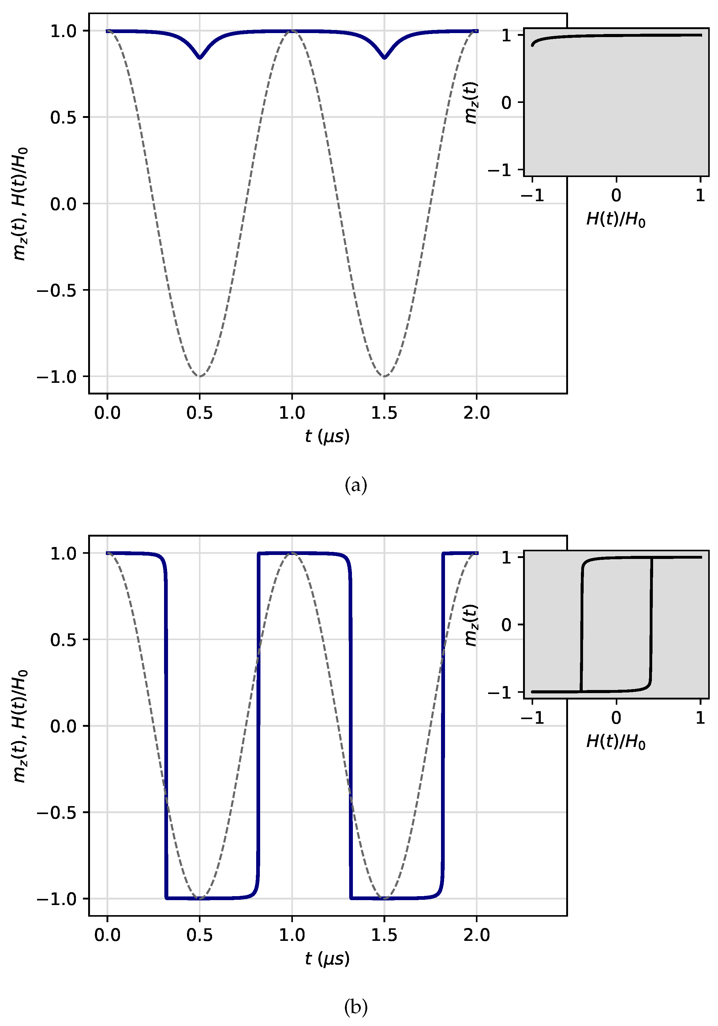
Figure 2.
Determination of the metastable lifetime corresponding to the first-passage time through zero magnetization from saturation state. The initial configuration corresponds to a fully saturated state along the main direction of the AMF. The parameters are Hz, mT and and orientation of the magnetic easy-axis relative to the field direction. The metastable lifetime in this case is s.
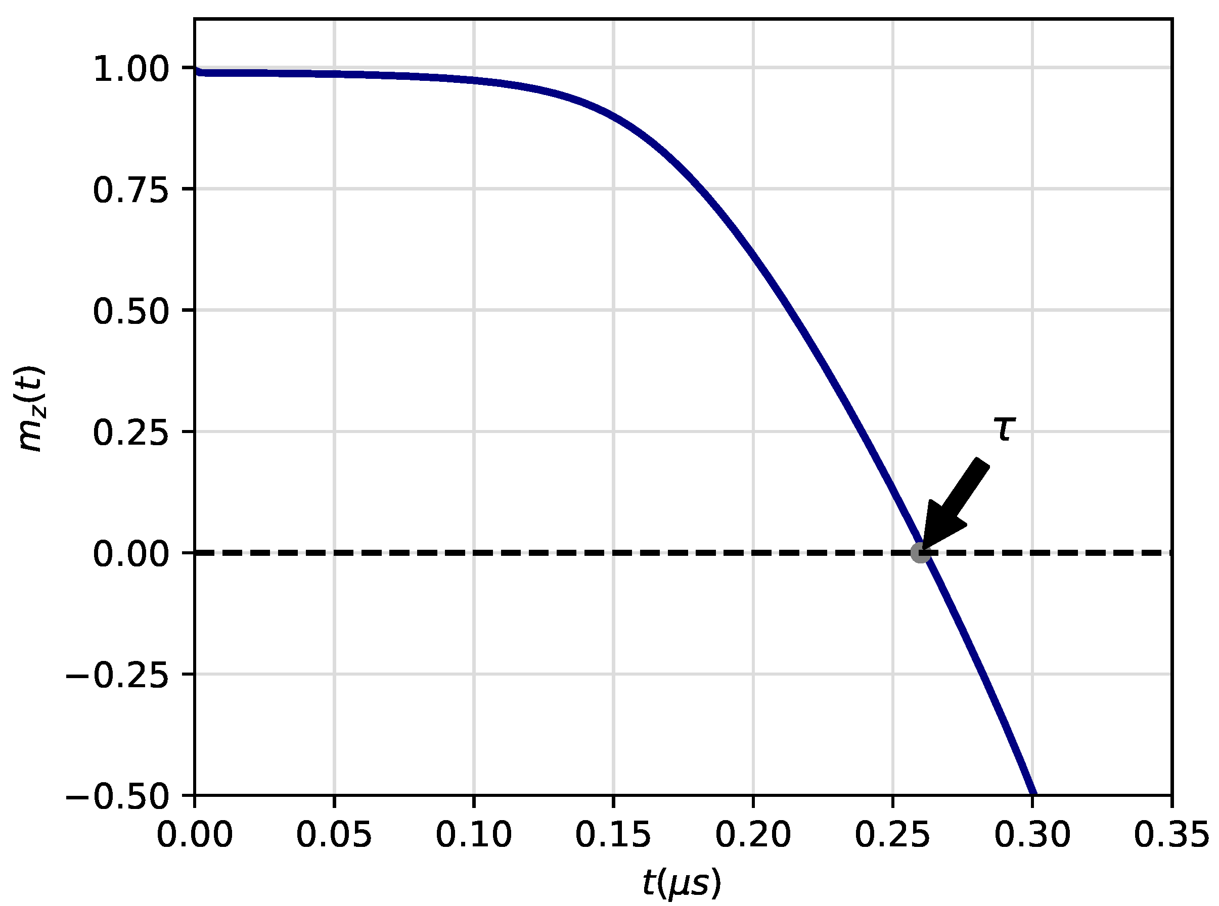
Figure 3.
(a) Finite-difference mesh used in our simulation. (b) Coordinates for the magnetic easy-axis orientation of the MNP. Where is the angle between the main direction of the external AMF and the magnetic easy-axis orientation.
Figure 3.
(a) Finite-difference mesh used in our simulation. (b) Coordinates for the magnetic easy-axis orientation of the MNP. Where is the angle between the main direction of the external AMF and the magnetic easy-axis orientation.
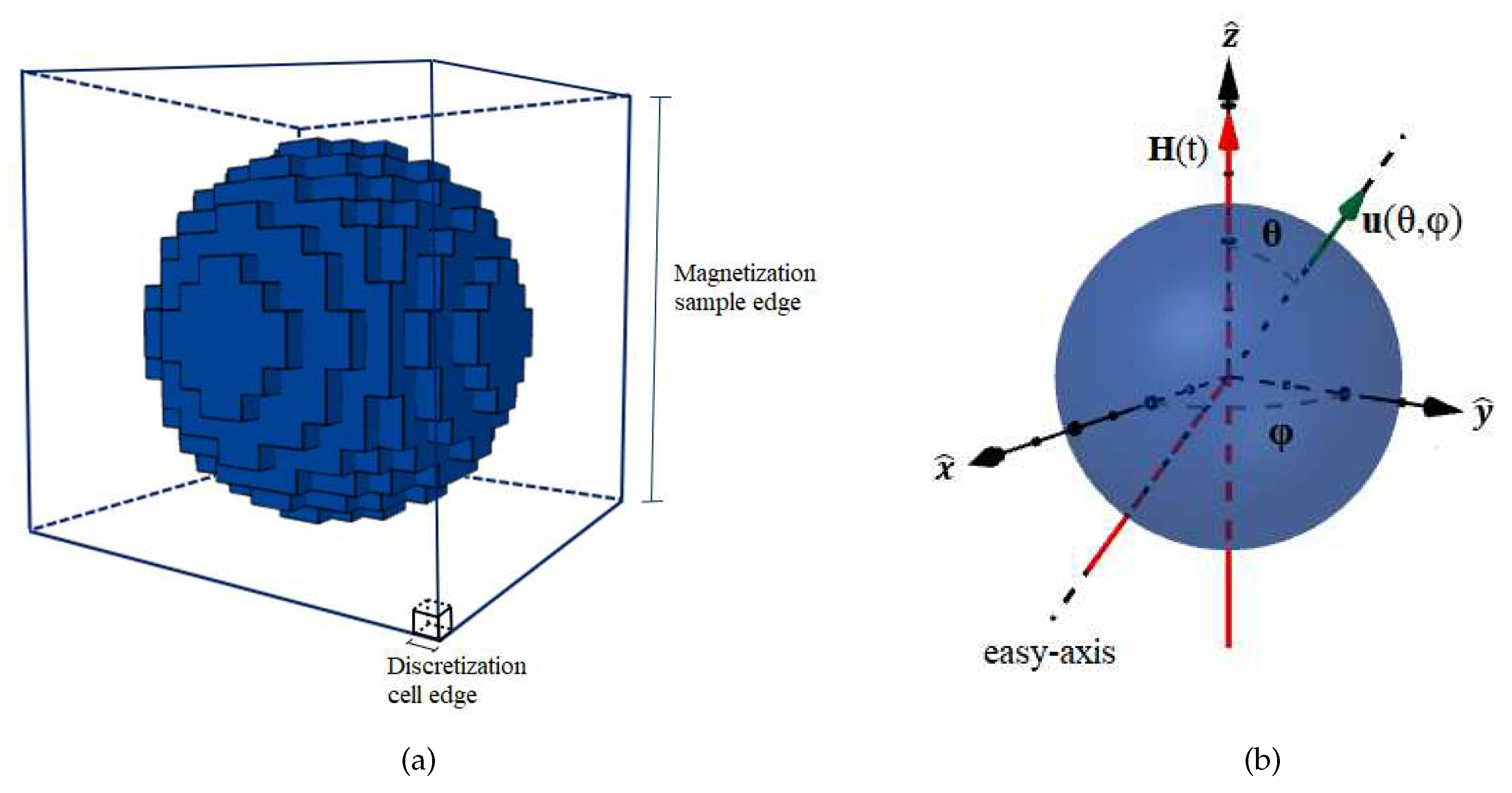
Figure 4.
Time dependence of the -component of magnetization and the external AMF. Polar angles for the easy-axis orientation are: (a) , (b) and (c) , for an amplitude of mT. Polar angles for the easy-axis orientation are: (d) , (e) and (f) , for an amplitude of mT. Figures (a)-(c) show a typical dynamic ordered phase (DOP) whereas figures (d)-(e) show a typical dynamic disordered phase (DDP).
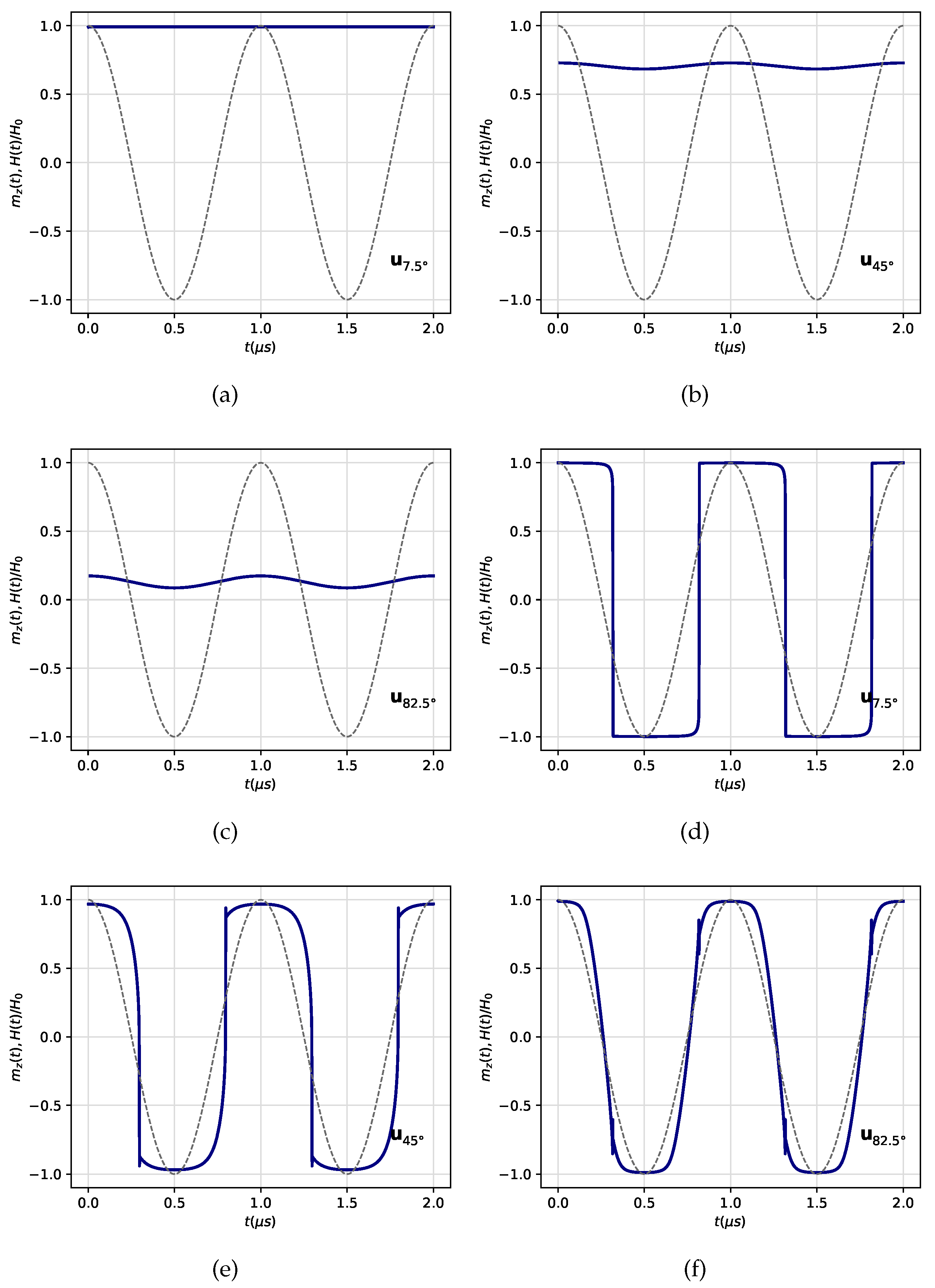
Figure 5.
Dynamic phase diagram between the DOP and the DDP. The coloured regions represent the DOP (pink) and DDP (violet) phases. Error bars are determined by the step of the AMF, namely mT.
Figure 5.
Dynamic phase diagram between the DOP and the DDP. The coloured regions represent the DOP (pink) and DDP (violet) phases. Error bars are determined by the step of the AMF, namely mT.
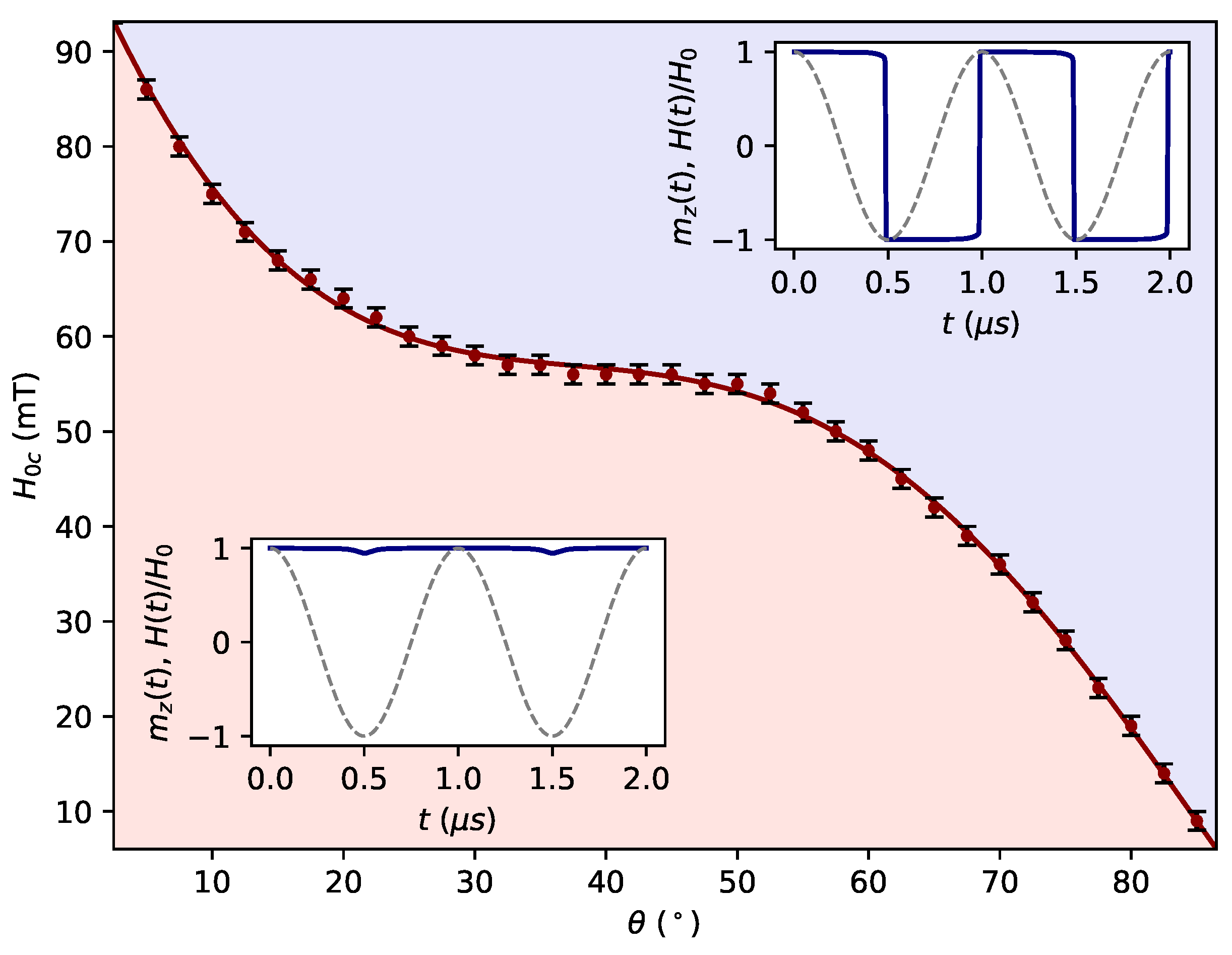
Figure 6.
Dependence of the metastable lifetime with the polar angle for mT.
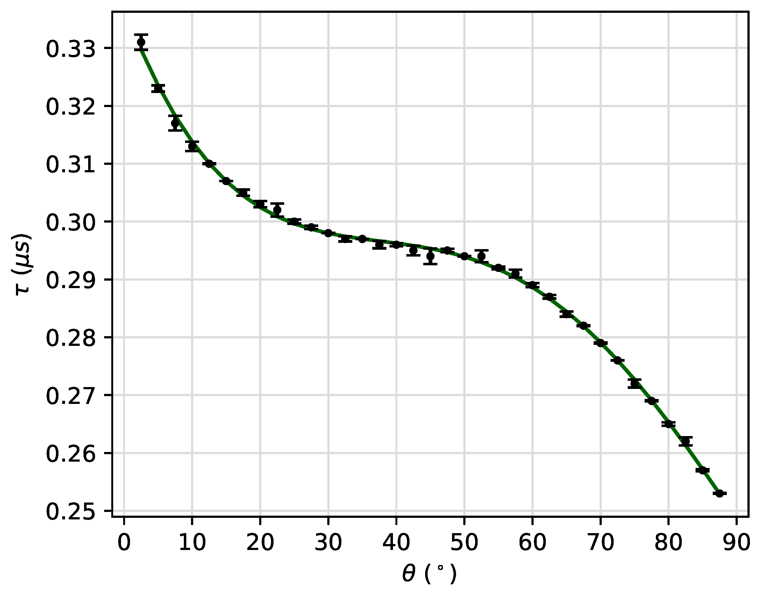
Figure 7.
Hysteresis loops for a field amplitude mT and for three different angles of the applied feld with respect to the easy-axis orientations of the MNP, namely , and . The ascending curves (from negative to positive saturation) are shown in orange, while the descending curves (from positive to negative saturation) are shown in black. For and , crossing of branches is evident.
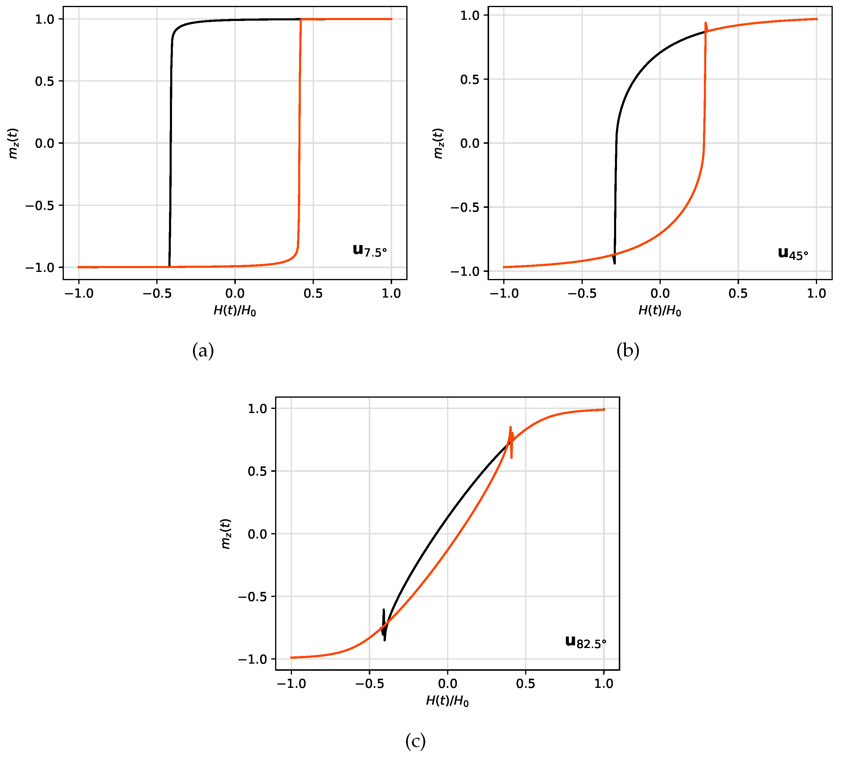
Figure 8.
Micromagnetic energy contributions as a function of the reduced applied field for different easy-axis orientations , and . (a-c) Exchange energy. (d-f) Demagnetization energy. (g-i) Anisotropy energy. (j-l) Zeeman energy. Orange lines stand for the ascending curves, while the descending curves are shown in black lines.
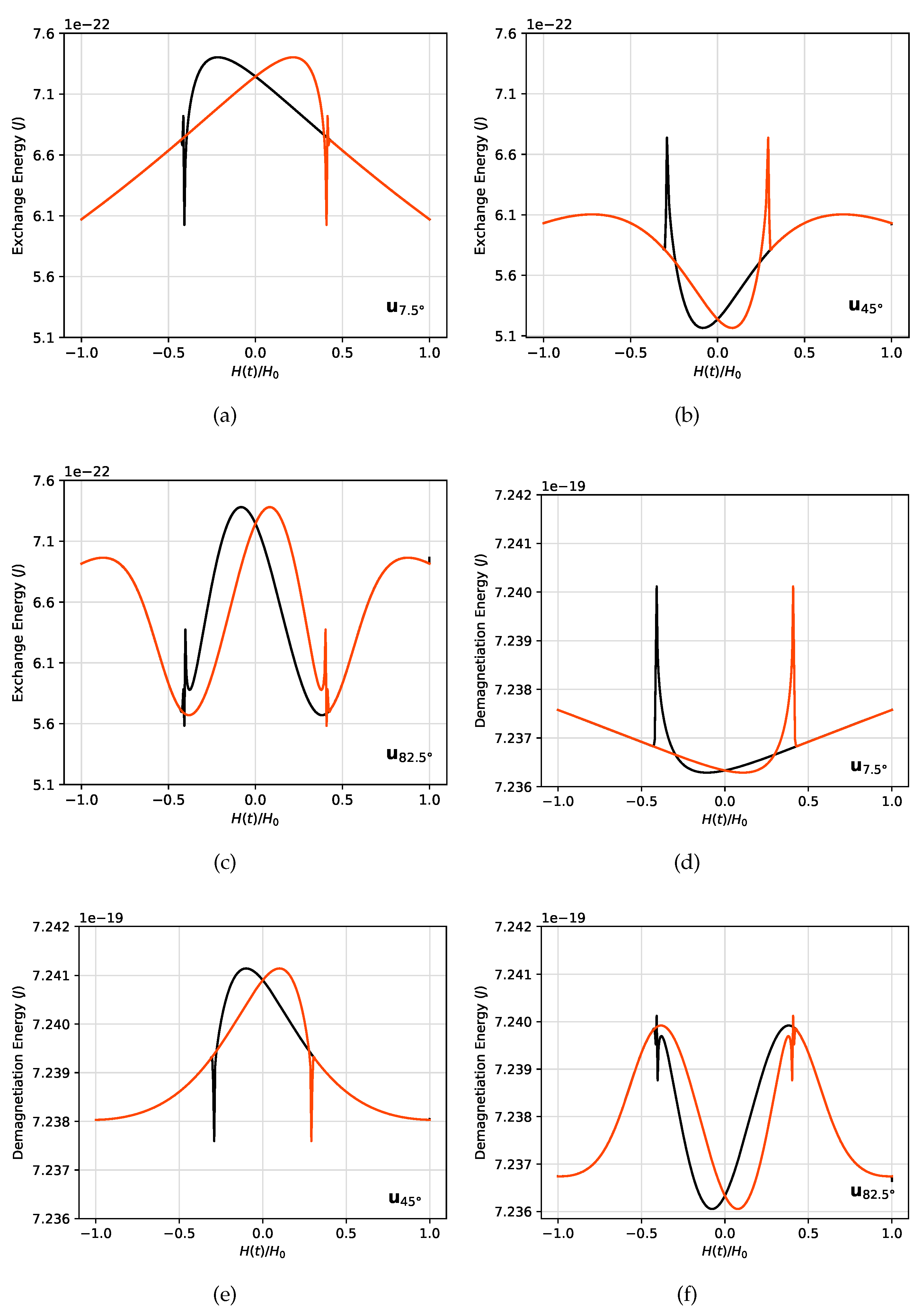
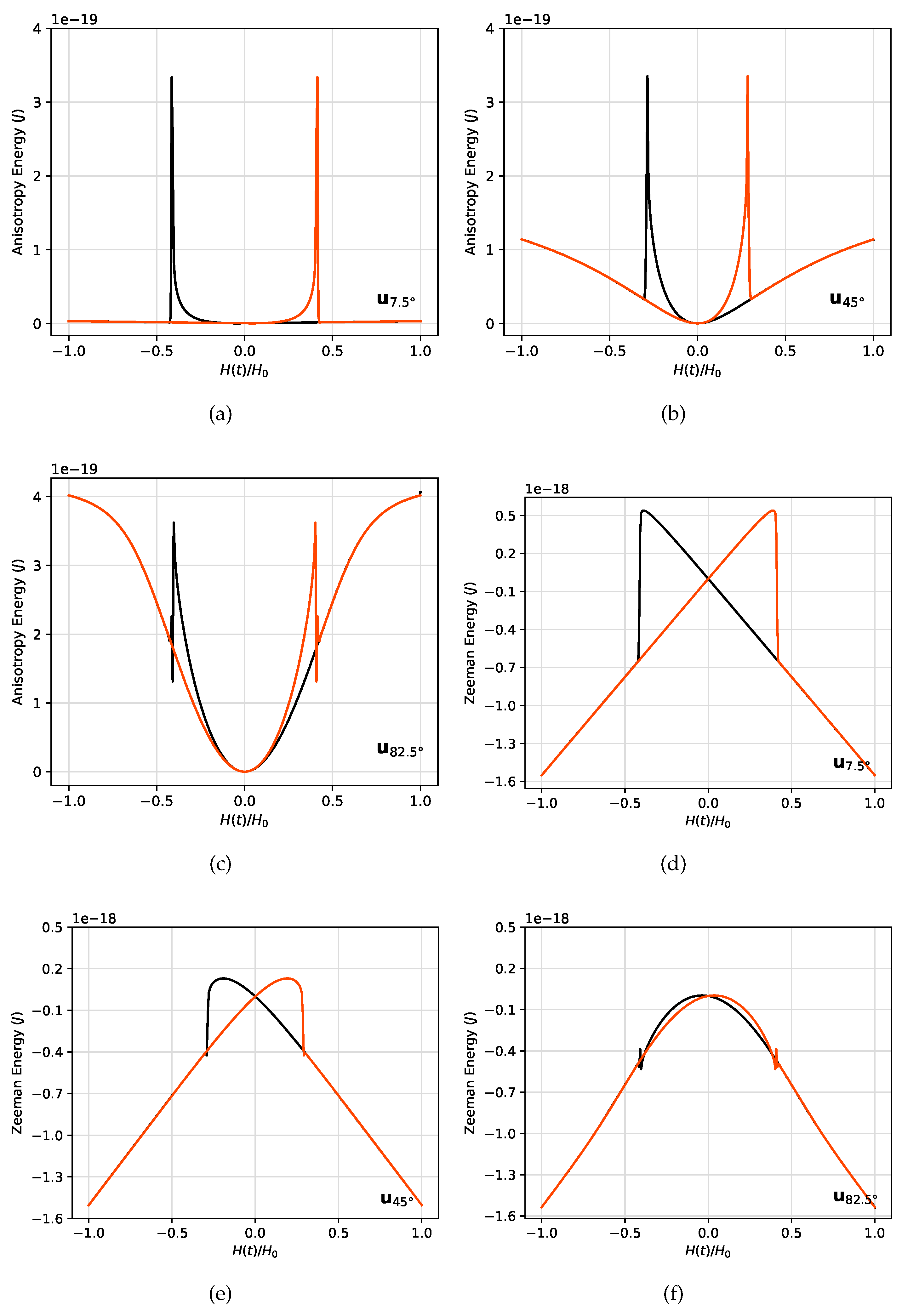
Figure 9.
Zoom of the (a-b) anisotropy and (c-d) Zeeman energies as a function of for . The ascending field branch is depicted in orange whereas the descending field branch is shown in black. At (red dashed line), (blue dashed line) and (green dashed line), energy contributions exhibit some jumps.
Figure 9.
Zoom of the (a-b) anisotropy and (c-d) Zeeman energies as a function of for . The ascending field branch is depicted in orange whereas the descending field branch is shown in black. At (red dashed line), (blue dashed line) and (green dashed line), energy contributions exhibit some jumps.
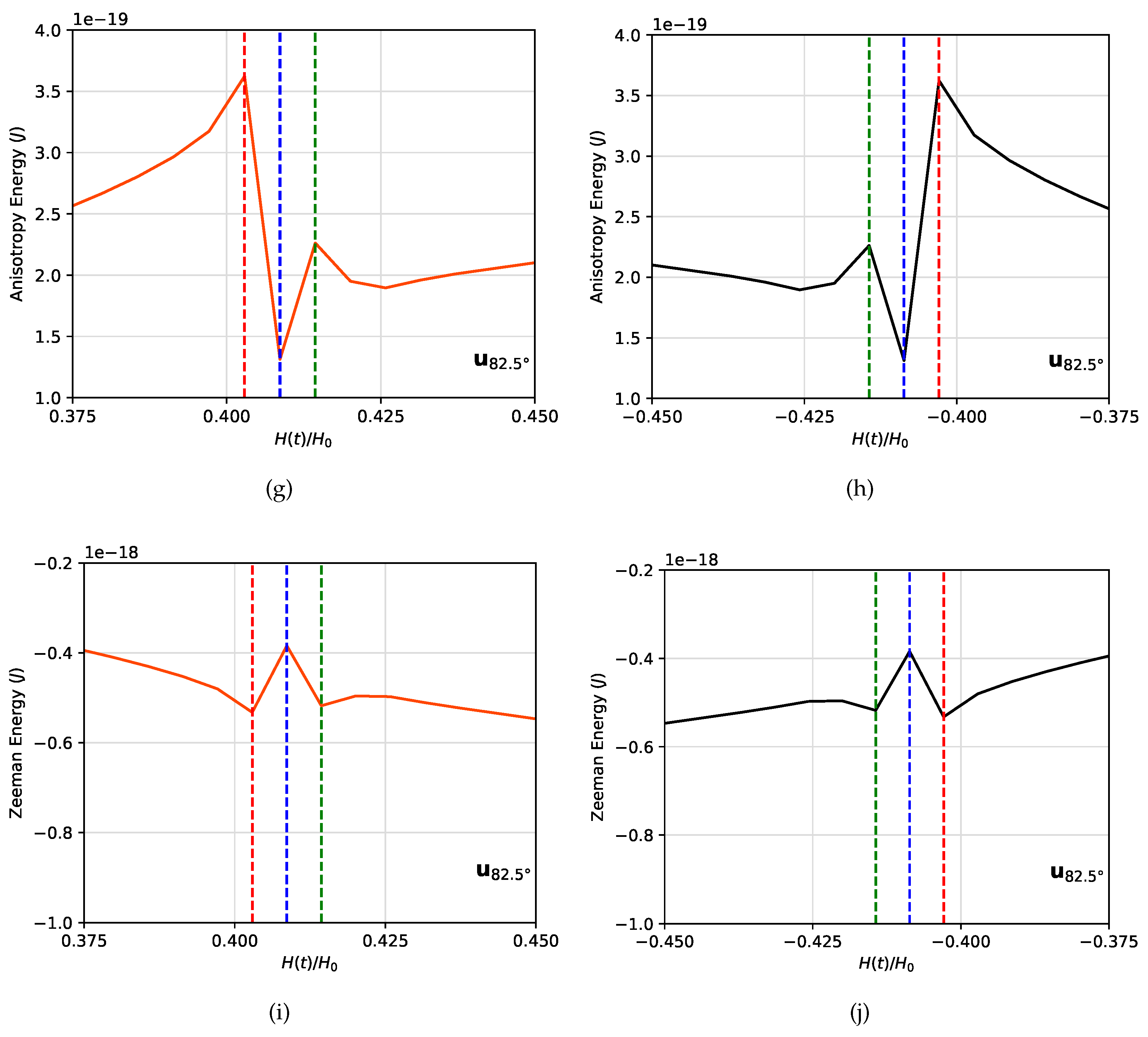
Figure 10.
Variation of the SLP as a function of the angle of easy-axis orientation for an amplitude mT of the external AMF.
Figure 10.
Variation of the SLP as a function of the angle of easy-axis orientation for an amplitude mT of the external AMF.

Disclaimer/Publisher’s Note: The statements, opinions and data contained in all publications are solely those of the individual author(s) and contributor(s) and not of MDPI and/or the editor(s). MDPI and/or the editor(s) disclaim responsibility for any injury to people or property resulting from any ideas, methods, instructions or products referred to in the content. |
© 2023 by the authors. Licensee MDPI, Basel, Switzerland. This article is an open access article distributed under the terms and conditions of the Creative Commons Attribution (CC BY) license (http://creativecommons.org/licenses/by/4.0/).
Copyright: This open access article is published under a Creative Commons CC BY 4.0 license, which permit the free download, distribution, and reuse, provided that the author and preprint are cited in any reuse.


