Submitted:
20 April 2023
Posted:
20 April 2023
You are already at the latest version
Abstract
To realize the diagnosis of compound faults in gearboxes at different speeds, an "end-to-end" intelligent diagnosis method based on a deep neural network is proposed, named efficiency channel attention-capsule network (ECA-CN). First, the process uses a deep convolutional neural network to extract fault features from the collected raw vibration signals, then embeds the efficient channel attention module to filter important fault features, then uses the capsule network to vectorize the feature space information, and finally calculates the correlation between different levels of capsules by the dynamic routing algorithm to achieve accurate gearbox compound fault diagnosis. The effectiveness of the proposed ECA-CN fault diagnosis method was verified by the composite fault dataset of the 2009 PHM Challenge gearbox, with an average accuracy of 99.63% and a standard deviation of 0.22%. In the comparison experiments with the traditional fault diagnosis method, the average accuracy of the ECA-CN method was improved by 4.62%, and the standard deviation was reduced by 0.58%. The experimental results show that ECA-CN has a more competitive diagnostic performance.
Keywords:
gearbox
; compound fault
; attention mechanism
; capsule network
1. Introduction
Gearboxes are one of the most widely used speed and power transfer elements in rotating machinery and play a vital role in manufacturing. Gearboxes contain gears, rolling bearings, drive shafts, and other components, which usually operate under harsh operating conditions with different speeds and loads and are prone to failures. And gearbox failure may lead to unexpected downtime, causing substantial economic losses and significant casualties. Therefore, it is essential to study gearbox fault diagnosis to ensure the efficient operation of mechanical systems [1].
Generally speaking, gears and bearings are the two components in gearboxes that are most prone to failure. Common failures include broken teeth, tooth surface wear, bearing fatigue spalling, and running wear [2]. And the loss of one component often causes the failure of another element in contact with it, triggering a compound failure. In the practical application of gearboxes, the features of solid faults easily cover the information of weak fault features due to the different damage mechanisms and loss degrees of individual defects embedded in the vibration signals [3]. Together with the complex transmission path of the movement, the vibration effects generated by different faults will interact, making the coupling and modulation phenomenon between the signals more severe and the mark features challenging to extract.
Traditional composite fault diagnosis methods usually use signal processing techniques such as wavelet transform analysis [4], resonance demodulation [5], and empirical modal decomposition [6,7] for feature extraction, and then shallow machine learning models such as BP neural networks [8] and support vector machines [9] for fault classification. Although the traditional methods have achieved fruitful results, the following drawbacks still exist in the era of big data [10]: 1) the process of feature extraction and selection using signal processing techniques is complex, requires manual operations, and relies mainly on engineering experience; 2) manual feature extraction reduces the complexity of the input data and causes rich fault state information to be lost in the original data; 3) the traditional signal feature extraction techniques make it difficult to separate the coupled features of compound faults.
Deep learning has been widely used in fault diagnosis, driven by artificial intelligence technology in recent years. Compared with traditional diagnosis methods, deep learning-based fault diagnosis methods are free from the reliance on expert knowledge and signal pre-processing methods, can directly excavate the composite fault features hidden in the original vibration signal, and have obvious advantages in the face of massive data. The convolutional neural network (CNN) is the most widely used among them. This is due to its features, such as local connectivity, weight sharing, and pooling operations, that can effectively reduce the number of training parameters, have strong robustness, and are easy to train and optimize. Yao et al. [11] proposed a CNN-based composite fault diagnosis method that converts bearing vibration signals into grayscale maps as training samples for the network, which can effectively identify bearing hybrid faults in urban rail trains. Zhang et al. [12] considered a deep convolutional generative adversarial network model under insufficient diagnostic samples and effectively improved the composite fault diagnosis by generating additional composite fault data samples. Sun et al. [13] combined an improved particle swarm-optimized variational modal decomposition with CNN to achieve mixed fault diagnosis of planetary gearboxes. Although the above methods achieved good results, each channel contains different information learned by the convolutional kernel for the features extracted by CNN. The traditional CNN gives the same weight to each track, ignoring the importance of the elements contained in different channels for the fault diagnosis task.
The attention mechanism considers the weight effect, i.e., the mapping relationship between input and output, which can enhance the key features and weaken the redundant components [14,15]. Therefore, introducing the attention mechanism into the diagnostic model can improve the effectiveness and reliability of the method. Li et al. [16] designed a fusion strategy based on the channel attention mechanism to obtain more fault-related information when fusing multi-sensor data features. Xie et al. [17] constructed an improved CNN incorporating the channel attention mechanism for fault diagnosis of diesel engine systems. The model mentioned above, considering feature weights, achieves good results, but scalar neurons reduce specific parameters such as location and scale in the feature mapping of their subject network CNN. Therefore, the fully connected layer requires a large amount of data to estimate the parameters of the features, and the demand for memory, computation, and data volume is enormous [18]. On the other hand, the pooling layer of the CNN gives the model a prior probability that is not affected b the translation but loses specific spatial information. In other words, CNNs obtain invariance rather than covariance [19].
In 2017, Sabour et al. [19] proposed a capsule neural network, which uses vectors to describe the object representation, where each set of neurons forms a capsule, and the capsule layer outputs vectors, with the vector length indicating the probability of the object presentation; the vector direction means the instantiation parameter. In mechanical fault diagnosis applications, multidimensional capsules can retain specific feature parameters at different rotational speeds. In addition, the capsule's distance represents the features' dispersion, so the capsule network's classification quality is better than traditional neural networks. Zhang et al. [20] combined wavelet transform and capsule network for bearing fault diagnosis in high-speed trains. Ke et al. [21] proposed an improved capsule network for the problem of insignificant composite fault features in modular multilevel converters.
The studies mentioned above only diagnose compound faults occurring in a single component, while in actual production, compound faults are usually coupled by multiple component faults in the transmission system. Therefore, an efficient channel attention capsule network is proposed for the problem of multi-component composite fault diagnosis in gearbox drive systems at different speeds. The method uses a one-dimensional convolutional neural network to extract composite fault features, introduces an efficient channel attention module to assign weights to the channel features, and performs composite fault classification by the capsule network. The main contributions of this paper are as follows: 1) ECA-CN discards the pooling layer in traditional CNN and introduces a capsule network instead, using a dynamic routing algorithm instead of pooling operation to ensure that the core features are not lost; 2) the activation function of ECA-CN is selected using GELU instead of the commonly used ReLU to accelerate the network convergence and effectively improve the robustness of the model; 3) the method does not require a time-consuming manual feature extraction process, and can achieve end-to-end gearbox composite fault diagnosis at different speeds.
2. Related Theory
2.1. One-dimensional convolution
In fault diagnosis, since the fault data is a one-dimensional vibrating signal, feature extraction is mainly performed using one-dimensional convolution. The role of the convolution layer is to convolve the local receptive domain of the input signal with the convolution kernel. Each convolution kernel extracts the local features of the input signal's local receiver domain under the activation function's action to construct the output feature vector. The output feature vector of each layer is the result of the convolution of multiple input features. The computational equation is as follows:
where: is the input signal of the th layer, is the weight matrix of the th convolution kernel of the th layer, is the bias, which is the eigenvalue extracted from the th convolution kernel of the th layer; denotes the activation function, and denotes the th element of the output eigenvector of the th layer.
The activation function enables the network to obtain nonlinear representation capability, enhance the feature representation of the model, map the initially linear and indistinguishable multidimensional features to another space, and make the features learned by the network more distinguishable. In recent years, rectified linear unit (ReLU) has been widely used as the activation function of the fault diagnosis model to accelerate the convergence of the model, and its calculation formula is as follows:
This paper uses the Gaussian error linear unit (GELU) [22], calculated as follows:
where: denotes the activation value input of the current neuron and denotes the cumulative distribution function of the Gaussian normal distribution . The differences between GELU and ReLU are shown in Figure 1. GELU not only solves the problem that ReLU is not controllable at the origin but also avoids the problem that the gradient disappears when the input is negative and improves the model expression capability of the model. In addition, it incorporates regularization, which allows stochastic regularization based on the probability that the current input is greater than the rest of the information, weighting the inputs according to their levels, which can maintain the uncertainty of the inputs and establish the dependence on the input values [23].
2.2. Capsule network
The core idea of a capsule network (CN) is to transform each neuron of a traditional neural network from scalar to vector and use a vector as the input and output of the network to reduce the loss of feature information and improve the feature extraction ability of the model. The mode length of the vector represents the probability of a particular health state of the gearbox occurring. The direction of the vector then means the information on the gearbox’s health state. The capsule network mainly consists of an initial capsule layer and a digital capsule layer, and the specific structure is shown in Figure 2.
The operation process of the capsule network is as follows:
Step 1: The initial capsule vector is multiplied with the weight matrix to obtain the predicted capsule , which can be expressed as (6):
Step 2: The prediction capsule is weighted and summed with the coupling coefficient to obtain the routing capsule , where the coupling coefficient is obtained through the intermediate variable , and the initial values are all 0:
Step 3: Compress the routing capsule using the Squash activation function, which can preserve the spatial information of the feature vector, i.e., keep the direction of the capsule vector unchanged, while compressing the modal length of the capsule to 0~1, to obtain the digital pill :
Step 4: Optimize the digital capsule by iteratively updating the parameters in the digital capsule layer using a dynamic routing algorithm. The correlation between the two is first calculated by predicting the inner product of the capsule and the digital capsule . The intermediate variable is optimized by:
Then is updated according to Eq (7). If the correlation between two capsules is high, the value of their coupling coefficient will increase, and vice versa will decrease. Subsequently, the dynamic routing is iterated through the formula, optimizing , . A total of iterations are taken in this paper as [19]. Finally, the optimal numerical capsule is obtained, whose direction indicates a particular health state of the gearbox, and the mode length indicates the probability of occurrence of this state :
2.3. Marginal loss function
In this paper, marginal loss (margin loss) is used as the loss function, which can effectively expand the difference between classes and reduce the difference within classes, and the calculation formula is as follows:
where: is the fault class, denotes the marginal loss of class fault, and denotes the probability value of the final output of the model. is the indicator function, means class fault exists, and means class fault does not exist. , are the upper and lower bounds, respectively. , in this paper, i.e., the loss value is 0 for or when the loss value is 0. is a scaling factor to adjust the ratio of these two items, and the matter taken here is 0.5.
3. Fault diagnosis method based on efficient channel attention capsule network
3.1. Efficient channel attention module
Efficient channel attention (ECA) [24] is a lightweight, plug-and-play attention module with good generalization capability to improve the performance of CNN architectures. The ECA module is processed as shown in Figure 3, given an input feature map , of size , where is the number of channels and is the width. Figure. 3 The schematic diagram of the efficient channel attention module.
Step 1: Aggregate the spatial information using global average pooling (GAP) to obtain the spatial information description vector :
Step 2: The is deformed and processed by one-dimensional convolution to achieve local cross-channel information interaction, and then the channel attention weight is obtained by the Sigmoid activation function. Where the size of the convolution kernel is adaptively selected according to the number of channels in the input feature map, calculated as follows:
where both are constants, and . indicates that the nearest odd number is taken.
Step 3: Multiply the deformation with to get the feature map corrected by channel attention.
3.2. Efficient channel attention capsule network
The architecture of the efficient channel attention capsule network constructed in this paper is shown in Figure 4, which mainly includes the input layer, convolutional layer, ECA module, initial capsule layer, digital capsule layer, and classification layer. The network processing process is as follows:
1) The vibration signal sample is input from the input layer, and the fault feature is finally obtained using one-dimensional convolutional step-by-step feature extraction. It is worth noting that the method uses wide convolutional kernels in convolutional layer 1, which can extract global features and reduce the effect of noise. And the kernel size of the subsequent convolutional layers is chosen as narrow convolutional kernels that become progressively smaller as the network level deepens, which can fully exploit the local features.
2) The ECA module assigns weights to the features of different channels in and obtains the attention-corrected feature map . Channel attention can enhance critical fault information, suppress useless information, and solve the feature redundancy problem.
3) In the initial capsule layer, five groups of convolution are performed on , which features can be further extracted. After convolution, the scalar values in the feature matrix are spliced to construct 320 initial capsules with a capsule dimension of 5. For the initial capsules, the spatial relationship is represented by each corresponding capsule because of the large number of pills. Since the initial and digital tablets are weighted mapping relationships, the number of digital capsules decreases, but the fault information embedded in each capsule increases. In the digital capsule layer, the dynamic routing algorithm is used to calculate the correlation between the initial capsule and the digital capsule, update the weights, complete the conversion between the pills to realize the accurate categorization of fault information, and finally generate six digital tablets with a capsule dimension of 10.
4) Calculate the two-parametric number of digital capsules to obtain the probability of different gearbox health states as in equation (11).
In this paper, compared with the traditional CNN fault diagnosis method, firstly, GELU is used as the activation function to introduce a nonlinear transformation to the network while adding random regularization, which makes the network converge faster and more robust. Secondly, the efficient channel attention module is introduced, which can assign weights to different fault information learned by the network, highlighting the fault information that plays a vital role in the diagnosis decision and suppressing the useless and harmful information, effectively solving the feature redundancy problem. Finally, the traditional pooling layer is discarded in favor of a capsule network using a dynamic routing algorithm. It thoroughly explores the fault features and maximally preserves their spatial information through vector neurons to obtain better fault diagnosis performance than the traditional CNN.
3.3. Fault diagnosis process
In this paper, CNN, ECA, and CN are combined to build a deep learning network that can be used for compound fault diagnosis of gearboxes under different speed conditions, and its diagnosis process is shown in Figure 5. The specific diagnosis steps are as follows:
1) Collect the vibration data of the gearbox at different rotational speeds using acceleration sensors.
2) Overlap sampling of vibration data is performed to obtain the training set. The leave-out method randomly divides the training set into a new training set and a validation set. To prevent the information leakage of the test set, the vibration data are routinely window sampled to obtain the test set.
3) Construct the ECA-CN model and initialize the parameters.
4) Train the model using the training set, select the optimal model based on the validation set, and save the model parameters.
5) Evaluate the final model using the test set and derive the diagnosis results.
4. Fault diagnosis method based on efficient channel attention capsule netw
4.1. Experimental Data Introduction
To verify the effectiveness and superiority of the method in this paper, the gearbox dataset from the 2009 PHM Challenge [25] is used as the experiment’s fault data. This dataset is divided into two groups: spur gears and helical gears, and the helical gear data is selected in this paper. The sketch of the gearbox structure is shown in Figure 6, which contains six bearings and three drive shafts, i.e., input, intermediate, and output shafts, where the gears on the output and input shafts have 16 and 40 teeth, respectively. The teeth of the two bags on the intermediate shaft are 48 and 24, respectively.
The vibration data were collected under the low load of the gearbox at 30Hz, 40Hz, and 50Hz, respectively, with a sampling frequency of 66.7Hz and a sampling time of 4s, and the time domain diagram of the collected signals is shown in Figure 7. In this experiment, the sampling window length is 2048, the overlapping sampling moving step is 500, 1500 samples are overlapped for each working condition, 600 samples are routinely sampled, all models and labels are detailed as shown in Table 1, and the six health states of the gearbox are described as shown in Table 2. The samples obtained from overlap sampling are randomly assigned into a training set and validation set, of which 8000 models are in the training set, 1000 samples in the validation set, and 1000 samples are randomly selected from the samples obtained from conventional sampling as the test set.
4.2. Ablation experiments
To verify the effectiveness of ECA-CN, it was compared with ECA-CN (ReLU) and a capsule network without ECA, i.e., CN (GELU). The parameter settings for this experiment are shown in Table 3.
Figure 8 shows the three models' training set loss and accuracy curves. Comparing ECA-CN with ECA-CN(ReLU), it can be seen that the loss curve and accuracy curve of the method in this paper converge faster. This is because GELU avoids the problem of gradient disappearance when the input is negative, and the expressiveness of the model is improved. GELU also has an adaptive Dropout function to enhance the robustness of the model. Compared with CN(GELU), it is evident that the method in this paper, which uses the ECA module, converges faster. The main reason is that the ECA module can assign weights to different channel features, which can focus the attention of the network on the critical fault information and give less weight to other news, thus improving the learning efficiency of the neural network, i.e., speeding up the convergence of the network.
Figure 9 shows the test set confusion matrix of the three models; Case1~Case6 denote the six gearbox health states respectively, the horizontal axis indicates the predicted working condition category, and the vertical axis denotes the actual working condition category. The diagonal orange area represents the prediction accuracy of each condition, and the remaining green space indicates the misclassification rate. The method’s accuracy in this paper is better than ECA-CN(ReLU) and CN(GELU) on each working condition, and the accuracy of the test set is 99.71%, 99.29%, and 98.51%, respectively, which proves that the method is feasible.
To further illustrate the method’s effectiveness in this paper, the t-distributed stochastic neighbor embedding (t-SNE) algorithm is used to map the feature maps output from each layer of ECA-CN to two-dimensional space for feature visualization, as shown in Figure 10. Observing the original vibration data and the t-SNE maps of the four convolutional layers, we can find that the feature clustering effect of the network layers becomes more and more evident as the network level becomes more profound, which indicates that the combined use of large convolutional kernels and small convolutional kernels is effective. It is worth noting that the clustering effect of the feature maps corrected by ECA is better than that of the feature maps of the fourth convolutional layer, which further verifies the effectiveness of the combination of ECA and CN. Finally, both the initial capsule and digital capsule layers achieve good fault feature clustering, further validating the proposed method's effectiveness for compound fault diagnosis of gearboxes under variable speed.
4.3. Comparison experiments
To verify the superiority of ECA-CN over convolutional neural networks and shallow machine learning models, it was compared with CNN [26], fully connected neural network (FNN) [26], support vector machine (SVM) [26], random forest (RF) [26], and wavelet transform-multi-label convolutional neural network (WT-MLCNNN) [27]. To avoid specificity and chance, ten parallel experiments were conducted with the experimental parameters set as shown in Table 3, and the obtained results are shown in Table 4.
The comparison results are shown in Figure 11, where the CNN and RF using frequency data as input achieved 99.33% and 97.24% accuracy, respectively. Similarly, the FNN and SVM using manually extracted frequency features as information gained 91.62% and 92.83% accuracy, respectively. Although all these shallow models achieve good diagnostic accuracy, they cannot achieve end-to-end fault diagnosis. In contrast, the method in this paper uses raw vibration data as input, and the average accuracy is 99.63% with a standard deviation of only 0.22%, which indicates that ECA-CN can effectively extract the composite fault characteristics of gearboxes at different speeds and can accurately achieve end-to-end fault diagnosis. Compared with WT-MLCNN, which also uses raw vibration data as input, its accuracy is only 94.02% with a standard deviation of 0.75%; the method in this paper shows a more competitive performance.
5. Conclusion
This paper proposes an intelligent diagnosis model with an efficient channel attention capsule network for compound fault diagnosis of gearboxes at different speeds, which can realize "end-to-end" intellectual fault diagnosis from raw vibration data to fault identification. The method uses a deep convolutional neural network to extract fault features, introduce s ECA module for feature filtering, and use a capsule network to retain the spatial information of features, which can achieve accurate fault diagnosis. The effectiveness and superiority of the method are verified using the 2009 PHM Challenge gearbox dataset: 1) the ECA-CN model uses GELU as the activation function, and the experimental results show that the ECA-CN (GELU) converges faster and is more robust than the ECA-CN (ReLU); 2) the ECA-CN model introduces the ECA module, and the experimental results show that the CN has an accuracy of 99.70%, while the accuracy of CN without the attention module is 98.68%, indicating that the ECA module can effectively improve the fault diagnosis accuracy of the model; 3) Compared with the shallow machine learning model and the traditional CNN model, the average accuracy of ECA-CN is improved by 4.62%, and the standard deviation is reduced by 0.58%, showing a more competitive fault diagnosis performance, which can achieve compound fault diagnosis of gearboxes at different rotational speeds.
Author Contributions
Conceptualization, X.Z., H.J. and Q.X.; methodology, X.Z. and Q.X.; software, Q.X.; validation, X.Z. and Q.X.; formal analysis, H.J. and J.L; investigation, X.Z.; resources, X.Z.; data curation, Q.X.; writing—original draft preparation, X.Z.; writing—review and editing, X.Z., Q.X., H.J. and J.L. All authors have read and agreed to the published version of the manuscript.
Funding
This research was funded by National Natural Science Foundation of China, grant number 51865054.
Data Availability Statement
There is no data sharing in this article.
Conflicts of Interest
The authors declare no conflict of interest.
References
- Zhao Z, Wu J, Li T, et al. Challenges and opportunities of AI-enabled monitoring, diagnosis & prognosis: A review[J]. Chinese Journal of Mechanical Engineering 2021, 34(1), 1–29.
- Chen Xuefeng, Guo Yanjie, Xu Caibin, et al. A review of wind power equipment fault diagnosis and health monitoring research[J]. China Mechanical Engineering 2020, 31(2), 15.
- Dingcheng, Zhang, Dejie, et al. Energy operator demodulating of optimal resonance components for the compound faults diagnosis of gearboxes[J]. Measurement Science and Technology 2015, 26(11), 115003-115003.
- Yuan, J. Separation and Extraction of Electromechanical Equipment Compound Faults Using Lifting Multiwavelets[J]. Journal of Mechanical Engineering 2010, 46(1). [Google Scholar] [CrossRef]
- Wang Huibin, Hep Changfeng, Meng Jiadong, Chen Guangyi, Wu Lixiao. A composite fault diagnosis method for rolling bearings incorporating Autogram's resonance demodulation and 1.5-dimensional spectrum[J/OL]. Journal of Vibration Engineering:1-11[2022-09-03].
- Wang ZJ, Wang JY, Zhang JP, et al. Complex fault diagnosis of gearboxes based on improved MOMEDA[J]. Vibration. Testing and Diagnosis 2018, 38(1), 6.
- Li L, H. An improved \\{EEMD\\ with multiwavelet packet for rotating machinery multi-fault diagnosis[J]. Mechanical Systems and Signal Processing 2013. [Google Scholar]
- Pi Jun, Liu Peng, Ma Sheng, et al. Fault diagnosis of aerospace bearings based on MGA-BP network[J]. Vibration. Test and Diagnosis 2020, 40(2), 9.
- Zhou, K., Wu, K., Sun, Y., et al. Fault diagnosis of refrigeration equipment based on data mining and information fusion[J]. Vibration. Testing and Diagnosis 2021.
- Wang H, Li S, Song L, et al. A novel convolutional neural network based fault recognition method via image fusion of multi-vibration-signals[J]. Computers in Industry 2019, 105, 182–190. [CrossRef]
- Yao Dechen, Liu Hengchang, Yang Jianwei, Li Xi, Cui Xiaofei. Research on compound fault diagnosis of urban rail train bearings based on deep learning[J]. Journal of Railway 2021, 43(06), 37–44.
- Zhang Y, Zhang Z, Shao F, et al. Composite Fault Diagnosis Based on Deep Convolutional Generative Adversarial Network[C]// 2020 Asia-Pacific International Symposium on Advanced Reliability and Maintenance Modeling (APARM). 2020.
- Sun G D, Wang Y R, Sun C F, et al. Intelligent Detection of a Planetary Gearbox Composite Fault Based on Adaptive Separation and Deep Learning[J]. Sensors 2019, 19(23), 5222. [CrossRef] [PubMed]
- Yang Z B, Zhang J P, Zhao Z B, et al. Interpreting network knowledge with attention mechanism for bearing fault diagnosis[J]. Applied Soft Computing 2020, 97, 106829. [CrossRef]
- Woo S, Park J, Lee J Y, et al. Cbam: Convolutional block attention module[C]//Proceedings of the European conference on computer vision (ECCV). 2018: 3-19.
- Li X, Wan S, Liu S, et al. Bearing fault diagnosis method based on attention mechanism and multilayer fusion network[J]. ISA transactions 2021.
- Xie Y, Niu T, Shao S, et al. Attention-based Convolutional Neural Networks for Diesel Fuel System Fault Diagnosis[C]// 2020 International Conference on Sensing, Measurement & Data Analytics in the Era of Artificial Intelligence (ICSMD). 2020.
- Tianyou Chen, Wang Z, Yang X, et al. A deep capsule neural network with stochastic delta rule for bearing fault diagnosis on raw vibration signals[J]. Measurement 2019.
- Sabour S, Frosst N, Hinton G E. Dynamic Routing Between Capsules[J]. 2017.
- Zhang Y, Jiang Y, Yang Y, et al. Unknown Compound Faults Diagnosis of High-Speed Train Based on Capsule Network[C]// 2019 IEEE 14th International Conference on Intelligent Systems and Knowledge Engineering (ISKE). IEEE, 2019.
- Ke L, Liu Y, Yang Y. Compound Fault Diagnosis Method of Modular Multilevel Converter Based on Improved Capsule Network[J]. IEEE Access 2022, 10, 41201–41214. [CrossRef]
- Hendricks D, Gimpel K. Gaussian Error Linear Units (GELUs)[J]. 2016.
- Cao X, Xu X, Duan Y, et al. Health Status Recognition of Rotating Machinery Based on Deep Residual Shrinkage Network under Time-varying Conditions[J]. IEEE Sensors Journal 2022.
- Wang Q, Wu B, Zhu P, et al. ECA-Net: Efficient Channel Attention for Deep Convolutional Neural Networks[C]// 2020 IEEE/CVF Conference on Computer Vision and Pattern Recognition (CVPR). IEEE, 2020.
- Phm data challenge 2009. Available from: <https://www.phmsociety.org/competition/PHM/09>.
- Jing L, Zhao M, Li P, et al. A convolutional neural network based feature learning and fault diagnosis method for the condition monitoring of gearbox[J]. Measurement 2017, 111, 1–10. [CrossRef]
- Liang P, Deng C, Wu J, et al. Compound Fault Diagnosis of Gearboxes via Multi-label Convolutional Neural Network and Wavelet Transform[J]. Computers in Industry 2019, 113(2), 103132. [CrossRef]
Figure 1.
The function image of ReLU and GELU.
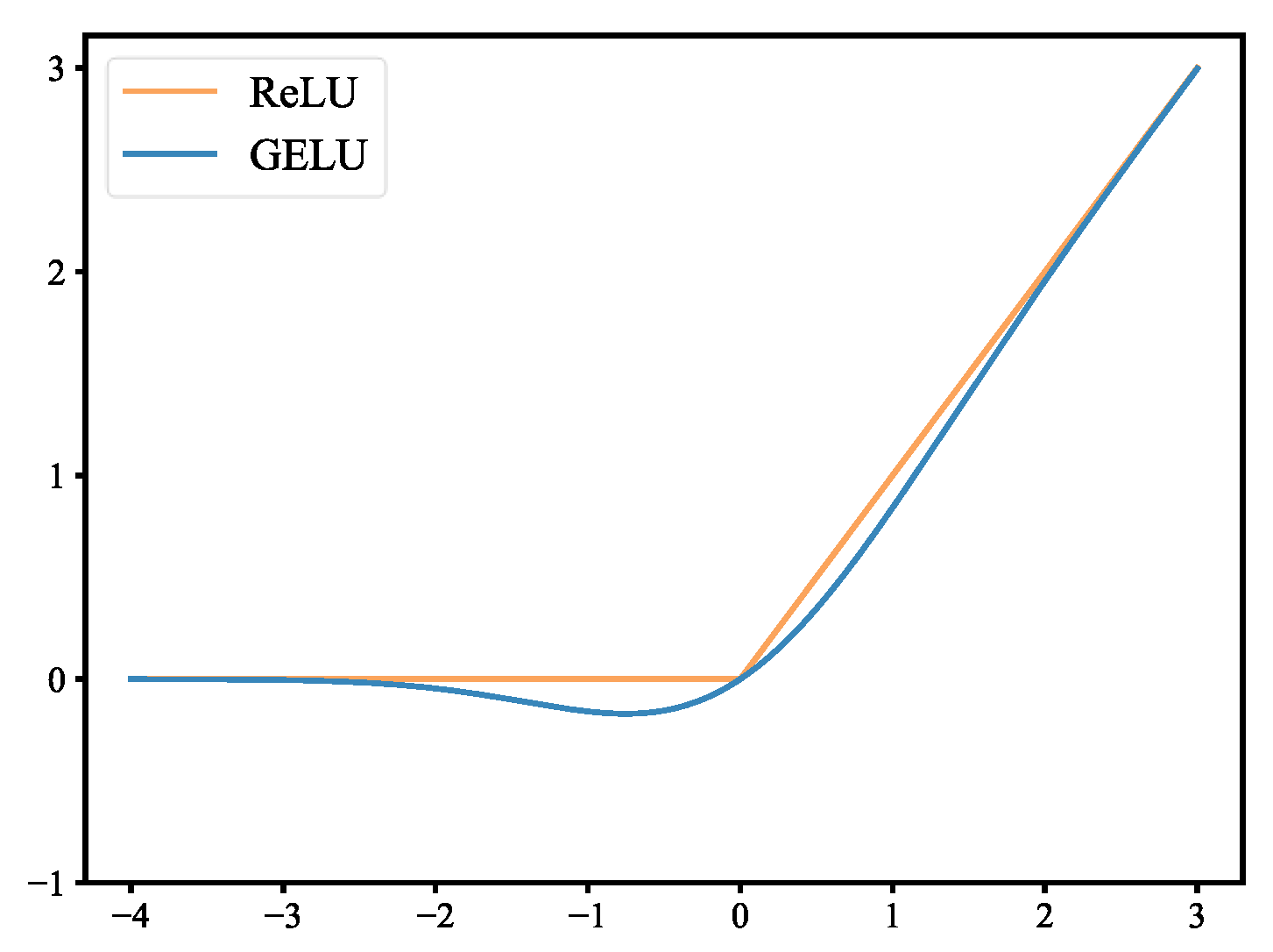
Figure 2.
The structure of the capsule network.
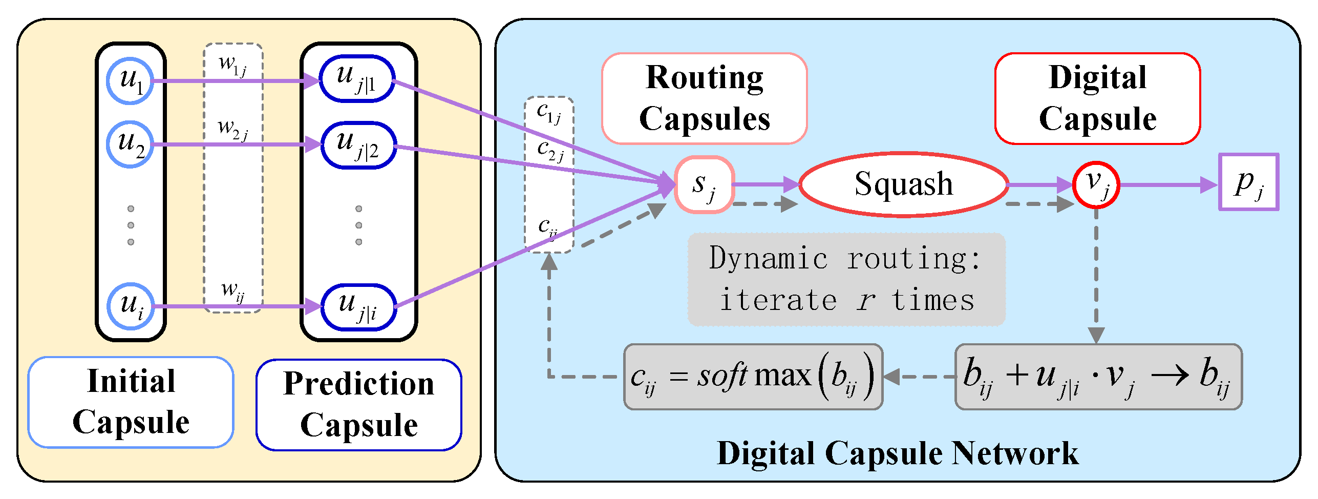
Figure 3.
The schematic diagram of the efficient channel attention module.
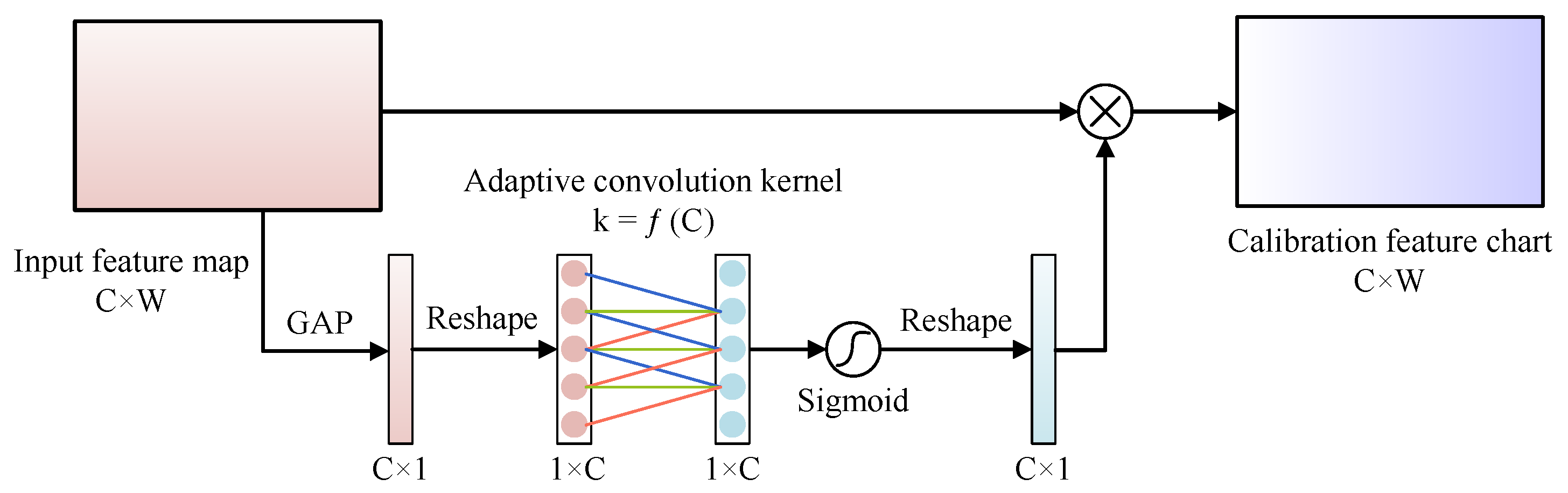
Figure 4.
The architecture diagram of the efficient channel attention capsule network.
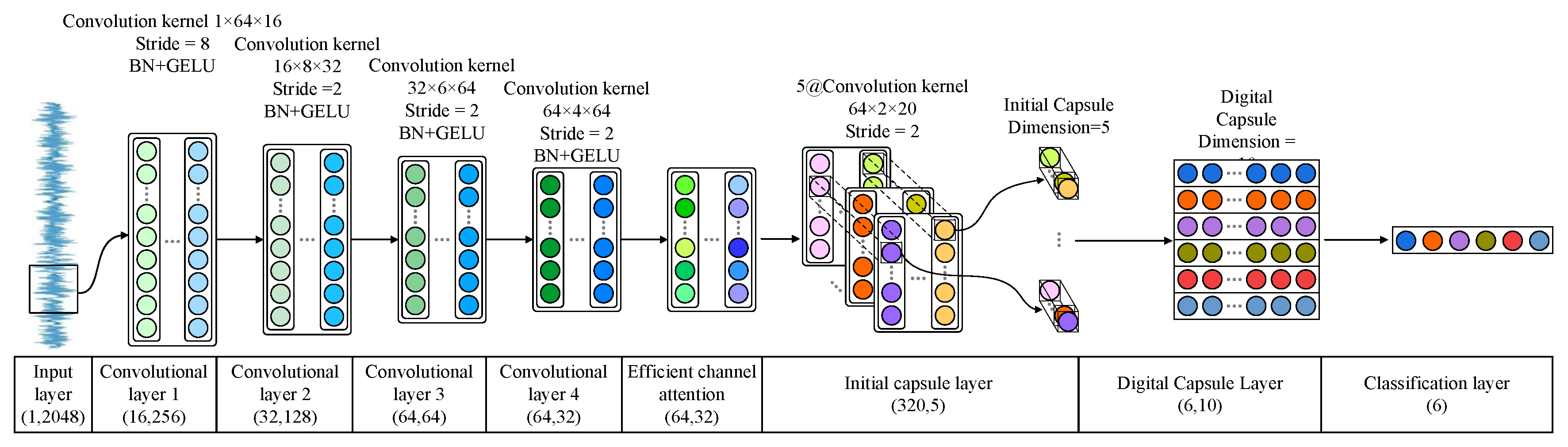
Figure 5.
The fault diagnosis process of ECA-CN.
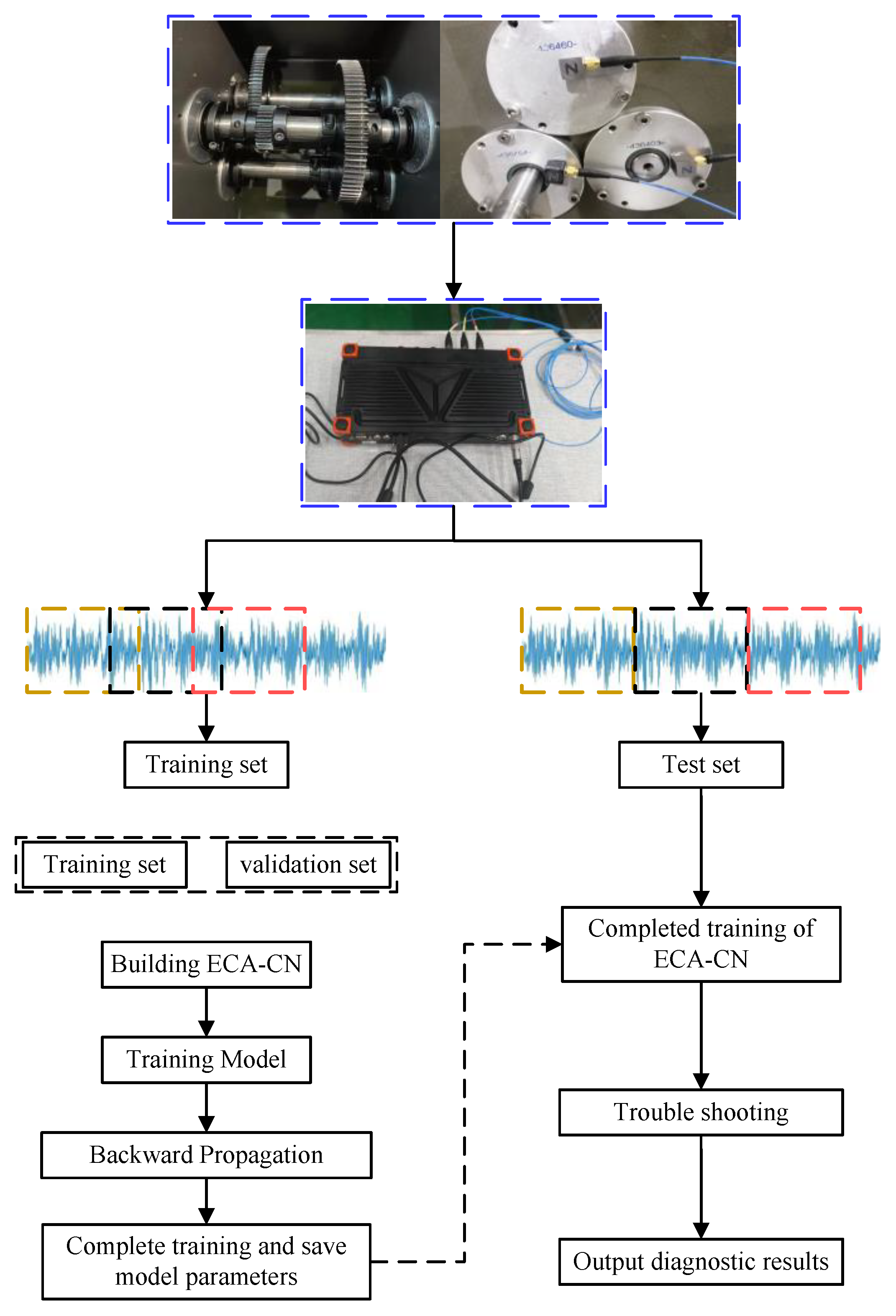
Figure 6.
The structural sketch of the gearbox.
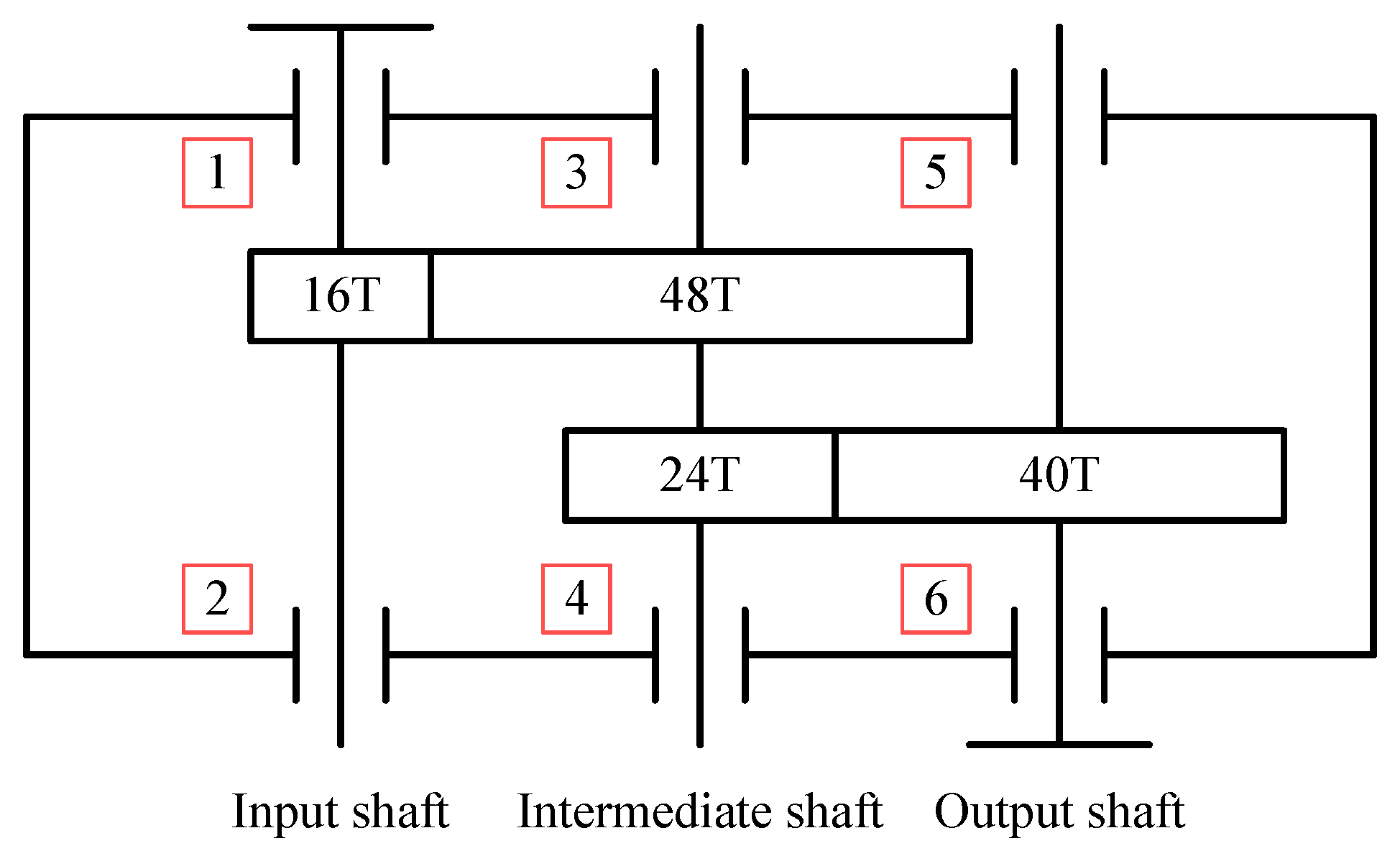
Figure 7.
The time domain diagram of vibration data.
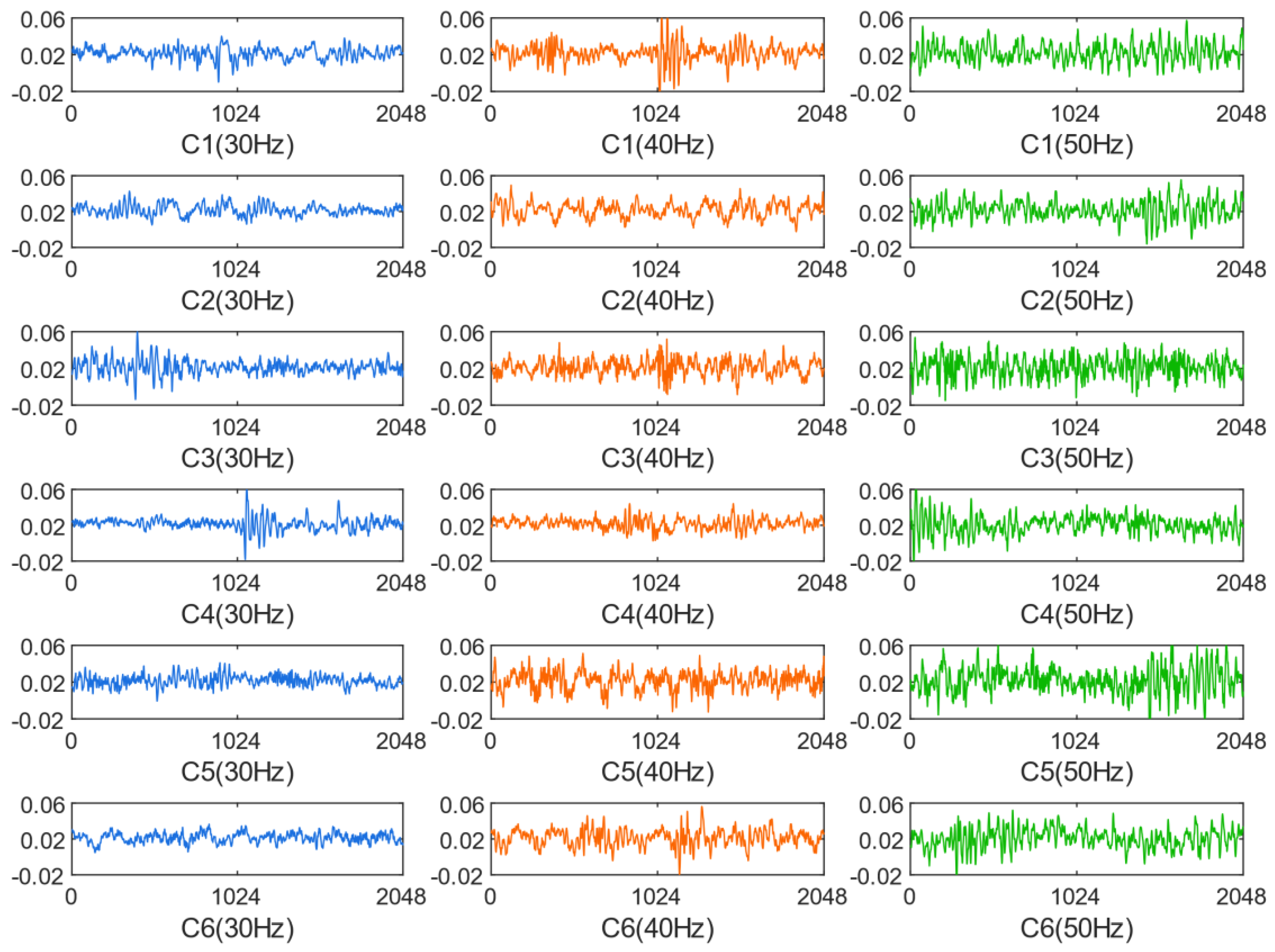
Figure 8.
Loss curve and accuracy curve. (a): Loss function curve; (b) Accuracy Curve.
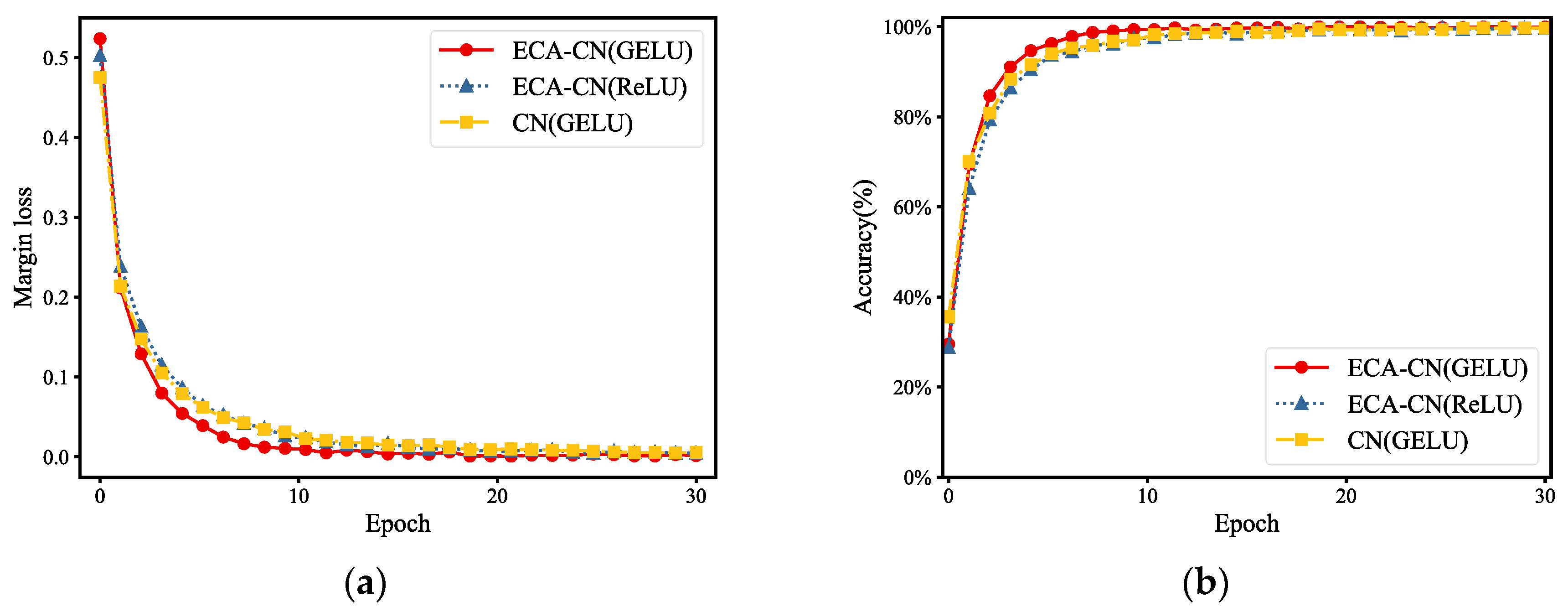
Figure 9.
The confusion matrix of the testing set. (a): ECA-CN (GELU) Test Set Confusion Matrix; (b) ECA-CN (ReLU) test set confusion matrix; (c): CN(GELU) test set confusion matrix.
Figure 9.
The confusion matrix of the testing set. (a): ECA-CN (GELU) Test Set Confusion Matrix; (b) ECA-CN (ReLU) test set confusion matrix; (c): CN(GELU) test set confusion matrix.
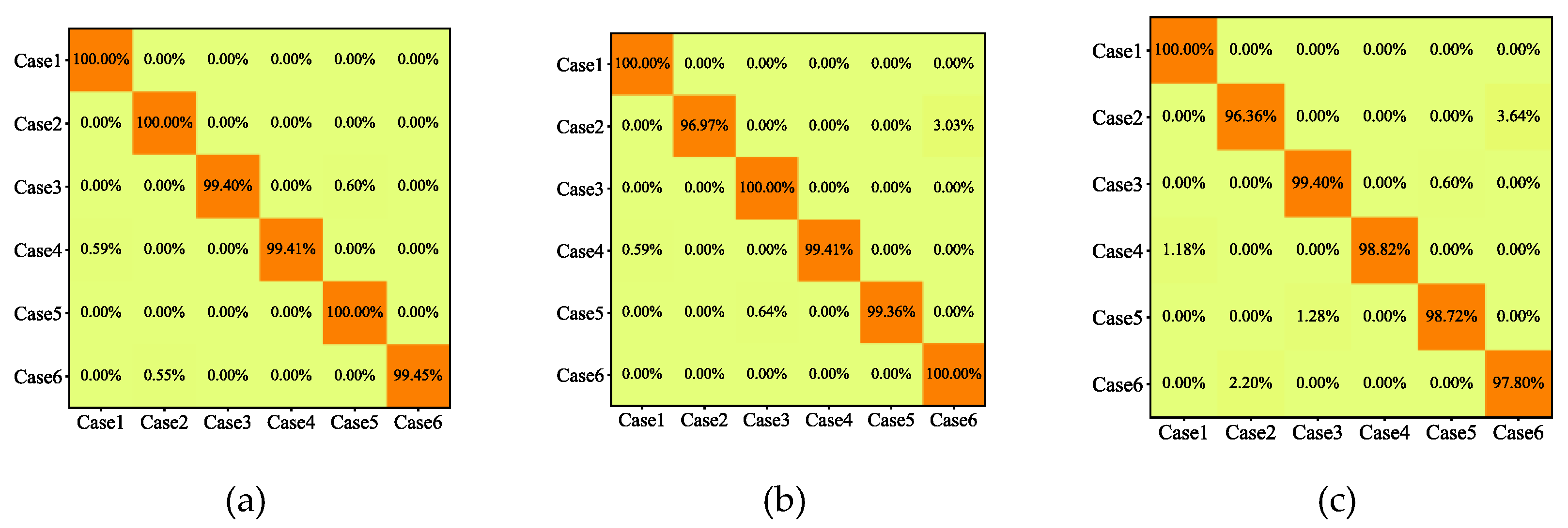
Figure 10.
t-SNE visualization of feature maps for each layer of the network. (a)Input layer; (b) First convolution layer; (c) Second convolution layer; (d) Third convolution layer; (e) Fourth convolution layer; (f) ECA Module; (g) Initial capsule layer; (h) Digital Capsule Layer.
Figure 10.
t-SNE visualization of feature maps for each layer of the network. (a)Input layer; (b) First convolution layer; (c) Second convolution layer; (d) Third convolution layer; (e) Fourth convolution layer; (f) ECA Module; (g) Initial capsule layer; (h) Digital Capsule Layer.
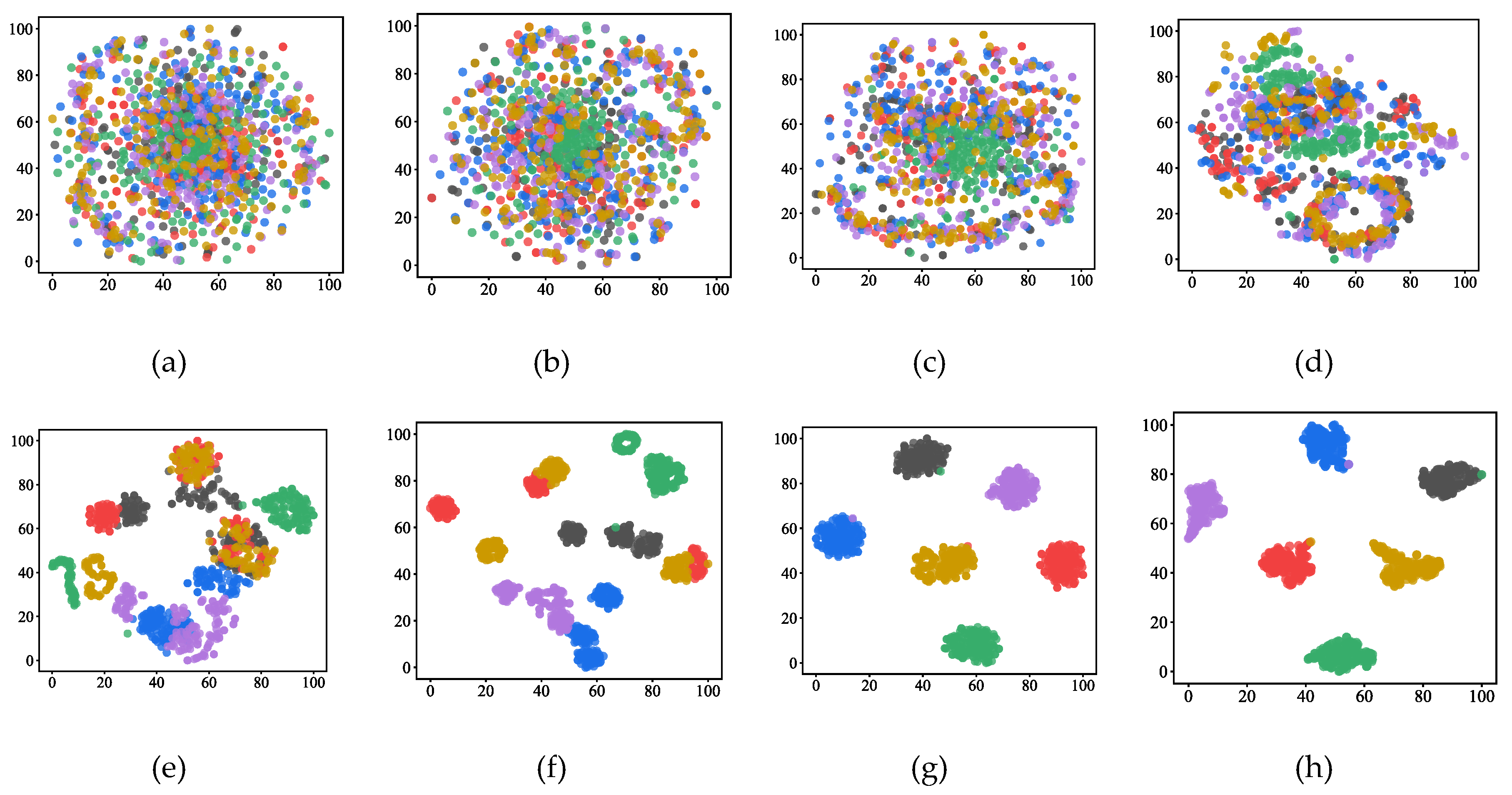
Figure 11.
Accuracy and standard deviation of each model.
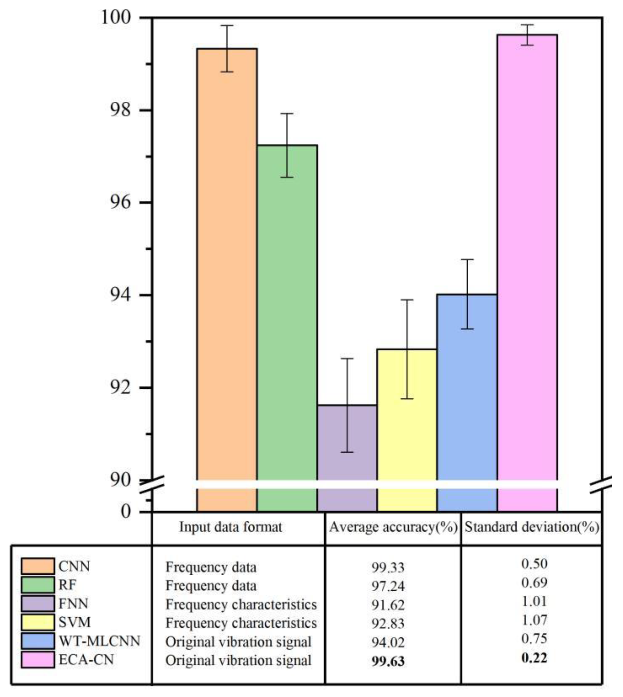

Table 1.
The description of samples and labels.
| Health Status. | Sample Length | Overlap Sampling | Conventional Sampling | One-hot label vector |
| 1 | 2048 | 1500 | 600 | [1,0,0,0,0,0] |
| 2 | 2048 | 1500 | 600 | [0,1,0,0,0,0] |
| 3 | 2048 | 1500 | 600 | [0,0,1,0,0,0] |
| 4 | 2048 | 1500 | 600 | [0,0,0,1,0,0] |
| 5 | 2048 | 1500 | 600 | [0,0,0,0,1,0] |
| 6 | 2048 | 1500 | 600 | [0,0,0,0,0,1] |
| 合计 | \ | 9000 | 3600 | \ |
Table 2.
The description of the gearbox’s health condition.
| Serial number |
Health Status |
Gear | Bearings | Shaft | |||||||||||
| 16T | 48T | 24T | 40T | 1 | 2 | 3 | 4 | 5 | 6 | Input | Output | ||||
| C1 | 1 | N | N | N | N | N | N | N | N | N | N | N | N | ||
| C2 | 2 | N | N | M | N | N | N | N | N | N | N | N | N | ||
| C3 | 3 | N | N | B | N | N | C | N | I | N | N | A | N | ||
| C4 | 4 | N | N | N | N | N | C | N | R | N | N | S | N | ||
| C5 | 5 | N | N | B | N | N | N | N | I | N | N | N | N | ||
| C6 | 6 | N | N | N | N | N | N | N | N | N | N | A | N | ||
M: missing tooth; B: broken teeth; C: composite fault; I: inner ring failure; R: rolling element fault; A: axis bending; S: shaft imbalance.
Table 3.
The experimental parameter setting.
| Parameter items | Parameter Setting |
| Loss function | Margin Loss |
| Sample Lot Size | 64 |
| Training rounds | 30 |
| Optimization algorithm | Adam |
| Learning Rate | 0.001 |
| Learning rate decay factor | 0.0001 |
Table 4.
The results of 10 parallel experiments of ECA-CN(%).
| Health Status | 1 | 2 | 3 | 4 | 5 | 6 | 7 | 8 | 9 | 10 | Average Accuracy Rate | Standard deviation |
| 1 | 100 | 100 | 100 | 100 | 100 | 99.37 | 100 | 100 | 100 | 100 | 99.93 | 0.19 |
| 2 | 99.39 | 99.39 | 100 | 98.18 | 100 | 98.79 | 99.39 | 100 | 99.39 | 100 | 99.45 | 0.57 |
| 3 | 99.40 | 100 | 100 | 98.21 | 100 | 100 | 100 | 100 | 97.62 | 100 | 99.52 | 0.83 |
| 4 | 100 | 100 | 99.41 | 99.41 | 99.41 | 99.41 | 99.41 | 100 | 99.41 | 99.41 | 99.58 | 0.27 |
| 5 | 100 | 100 | 99.36 | 99.36 | 100 | 99.36 | 99.36 | 100 | 100 | 99.36 | 99.68 | 0.32 |
| 6 | 100 | 99.45 | 98.90 | 100 | 99.45 | 100 | 100 | 99.45 | 99.45 | 100 | 99.67 | 0.36 |
| Test set | 99.79 | 99.80 | 99.61 | 99.19 | 99.81 | 99.48 | 99.69 | 99.90 | 99.31 | 99.79 | 99.63 | 0.22 |
Disclaimer/Publisher’s Note: The statements, opinions and data contained in all publications are solely those of the individual author(s) and contributor(s) and not of MDPI and/or the editor(s). MDPI and/or the editor(s) disclaim responsibility for any injury to people or property resulting from any ideas, methods, instructions or products referred to in the content. |
© 2023 by the authors. Licensee MDPI, Basel, Switzerland. This article is an open access article distributed under the terms and conditions of the Creative Commons Attribution (CC BY) license (http://creativecommons.org/licenses/by/4.0/).
Copyright: This open access article is published under a Creative Commons CC BY 4.0 license, which permit the free download, distribution, and reuse, provided that the author and preprint are cited in any reuse.


