
Submitted:
13 April 2023
Posted:
13 April 2023
You are already at the latest version
Abstract
The link of fracture analysis of large ships is an essential part of the structural safety of ships. However, the finite element analysis of large structure according to the traditional method not only has high requirements on the computer, but also the influence of the mesh encryption at special locations makes further requirements on the accuracy of the ship. In this paper, based on the extended finite element method (XFEM) and the multi-point constraint method (MPC), the dynamic crack expansion process of the rectangular plate containing cracks under the multi-scale model is comparatively studied by using ABAQUS simulation software Finally, the applicability of the method is verified by applying the multi-scale model of ship nodes. The results show that the computational effort of the multi-scale model is significantly reduced with the same accuracy and allowable error, which proves the accuracy and efficiency of the method.
Keywords:
Extend the finite element
; multi-point constraint
; ship crack
1. Introduction
The fracture problem [1] is something that will be inevitably encountered in production practice, and in the ship structure, the impact of cracks on structural damage is more involved in the huge economic interests of the nation, and the scale of the ship [2] has been gradually rising in recent years, and the corresponding maintenance cost for the ship is rising year-on-year, and the fracture problem of large scale ships is becoming more and more serious.
In the study of crack extension, the most representative numerical methods are: Finite Element Method [3,4,5,6], boundary element method [7,8] etc. However, these methods have certain problems in solving large scale ship fracture problems, for example, the traditional finite element must consider the defects inside the object when dividing the mesh, making the cell boundary consistent with the geometric boundary, which inevitably forms a local mesh encryption, and the rest This inevitably results in a non-uniform mesh distribution of the regional coefficients, which greatly increases the computational cost, and therefore it is difficult to balance the computational cost and the computational scale when solving the local fracture problem of some large ships. For the drawbacks of finite element treatment of discontinuous interface problems such as cracks, the extended finite element method [9,10,11] is a more optimal solution. In XFEM, the discontinuous crack surface and the computational mesh are independent of each other, and the division of cells does not depend on the geometric interface of the crack, and the mesh should not be re-divided after the crack is extended, so that the discontinuous mechanics problem [12] can be analyzed conveniently.
However, large scale problems also need to be considered together, and in order to meet the requirements of both computational efficiency and computational accuracy, it is necessary to split the large components and ensure the effective connection of interfaces between different scales, and the interface connection methods are transition unit method and multi-point constraint equation method, of which the transition unit method requires the establishment of different transition units for different units and different connection types, which leads to this type of The transition unit method has more types of transition units, and it is difficult for the finite element software to cover all of them, and the calculation accuracy at the interface is not high, but also prone to shear self-locking and other phenomena. In contrast, the multi-point constraint method can realize various assembly contact and motion constraints. It can also realize the connection between discontinuous and uncoordinated meshes of degrees of freedom, the connection between different cell types and other purposes, which provides a theoretical basis for the study of large scale ship fracture problems.
In this paper, the nodal model of a large scale ship is simplified based on the extended finite element theory (XFEM) and combined with the multi-point constraint theory [13,14,15] (MPC), and the cracks in the nodes of the ship are investigated using ABAQUS software, and the applicability of the method is verified using the stress intensity factor [16].
Simulation Procedure
2.1. Extended Finite Element Fundamental Theory
In conventional FEM, cracks or any other discontinuities are defined as an intrinsic part of the finite element mesh and are modeled by aligning the cell boundaries with the crack geometry. Therefore, as the crack tip advances, the mesh must be redefined to ensure alignment. In the XFEM method, the crack is mesh-independent, so the crack can propagate through the cell without remeshing. This significantly reduces computational resources. the XFEM method is based on three main factors: the non-smooth solution property, the unit decomposition, and the enrichment function. Non-smooth solution properties are properties that undergo rapid changes in the domain. These properties are associated with discontinuities, such as cracks, grain boundaries, holes, inclusions, etc. In practical applications, these discontinuities can be observed frequently and are usually divided into two categories: weak discontinuities (locations where the field quantities change direction) and strong discontinuities. The current research focuses on strong discontinuities. In XFEM, the traditional finite element approximation is improved by introducing discontinuities in the problem using an extrinsic PU method. In the last two decades, XFEM has been widely used to model crack growth [17]. Cracks in the XFEM mesh are defined by enriching the elements with additional degrees of freedom. The shape function in the finite element follows the PU property. This property states that the sum of the shape functions [18] of a particular element remains uniform at all locations within the specified element.
The step function [19] is chosen as the expansion of the displacement function for the crack surface discontinuity, and the step function is equal to 1 on one side of the crack and -1 on the other side of the crack, for the additional degrees of freedom of the unit nodes penetrated by the crack.
In the extended finite element, the finite element approximation of the unknown field [20] consists of two parts:
Where r and is the position parameter defined in the crack tip polar coordinate system, using this function base to construct the crack tip expansion shape function [21] can not only express the discontinuity of the displacement behind the crack, but also accurately capture the crack tip displacement field
The extended finite element method provides a more accurate description of complex unknown fields (e.g., intermittent displacement fields in the case of cracks) by adding expansion terms to the standard field approximation. In the extended finite element, the enrichment function [22] is added to provide a specific description of the displacement field, thus enabling the crack and mesh to exist independently in the form of
where S, is the set of nodes, is the set of fully penetrated unit nodes, is the set of split-tip unit nodes, and is the shape function of the corresponding node. The enrichment of nodes near the cracks is shown in Figure 1.
The third part is the finite element solution of the crack tip part,, reacting to the main singularities of the crack tip and various possible displacement states, where is the additional degrees of freedom of the crack tip unit, as a linear combination of the following function bases:
To simulate crack extension in Abaqus [23] using XFEM, damage sprouting and evolution [24] were considered. In this study, the maximum principal stress criterion [25] was used for damage sprouting. Damage will start when the principal stress exceeds the maximum principal stress value specified as part of the material property. For damage evolution, Abaqus used the scalar damage parameter [26] D to predict damage to the metal matrix due to nucleation, growth and agglomeration of micropores. It increases monotonically with plastic deformation and ranges from 0 for undamaged samples to 1 at complete failure. The damage stress (σ) using the damage factor is defined as :
where is the equivalent force in the undamaged model that takes into account the plastic behavior prior to necking. The damage evolution can be defined using the displacement at failure (the difference between the displacement at failure and the displacement at the onset of damage) or the fracture energy [27] (the area of the curve under the load versus displacement curve). In the current study, the displacement at failure was used as a parameter to define the damage evolution. The damage variables were calculated using the following equation :
2.2. Determination of stress intensity factor
The stress intensity factor [28,29] is an important physical quantity used in linear elastic fracture mechanics to reflect the strength of the stress field near the crack tip, which represents the strength of the stress field and is influenced by the geometry of the crack and the crack body and the external loading conditions. The stress intensity factor controls the magnitude of the stress, displacement, and strain fields at the crack tip, but the expressions differ slightly for the specific circumstances of each crack.
For the description of the change in the total energy of the system due to pre-existing crack formation, the description of the total energy release provided by the interaction integral [30,31] is more reasonable than the description of the energy release rate, and therefore it is more advantageous to use the interaction method to find the stress intensity factor.
The interaction method is derived from the J-integral [32], which is based on the principle that the cracked body not only bears the real load, but also bears the hypothetical auxiliary load, and the two act together on the cracked body, and in elastodynamics we can learn that the composite field formed by the superposition of the real field and the auxiliary field satisfies the superposition principle, and the addition between them will form a new J-integral composite field. The real field and the auxiliary field are brought into the J-integral to get their interaction integral terms, and after separating the J-integral caused by each of the composite field, the remaining real field and the auxiliary field corresponding to the interaction integral term is the interaction integral. The form is
The interaction integral can be solved by the given auxiliary field function and the real field function given by the extended finite element method, and the relationship between the J-integral and the stress intensity factor, which interacts with the stress intensity factor according to the superposition principle, is
By integrating the stress displacement function obtained from the extended finite element approach with the stress displacement function of the auxiliary field and the interaction integral, we have now successfully solved the stress intensity factor.
2.1.3. Multi-point constraints
In order to connect the critical parts of fine units and non-critical parts of macroscopic units at the same time, the parallel consistent multi-scale method can solve this problem, and this modeling method can take into account the influence of node fine damage on the overall force during the overall analysis, so it is more reasonable than the traditional single-scale modeling. However, this multi-scale modeling method requires high modeling accuracy at the interface coupling of units at different scales, and if the force transfer between units at the coupling is not reasonable, the simulation results of the critical parts obtained are meaningless, so the reasonable selection of the connection method between different interfaces becomes the key to the accuracy of multi-scale modeling.
The multi-point constraint method is used here, and since the most essential connection between different scale models at the interface should be the displacement relationship between the nodes at the interface, the constraint equation can be found by coupling the displacement of macroscopic and fine unit nodes at the interface connection. Combined with the finite element analysis software ABAQUS, the macroscopic and fine cell coupling can be realized by multi-point constraint equations, whose unified form can be written as
where is the displacement vector at the interface connection of macroscopic cells; is the displacement vector at the interface connection of fine cells, and is the coefficient matrix of the interface connection constraint equation.
In the specific derivation process of the constraint equation, certain simplifications and assumptions make the advantages and disadvantages of the two methods complement each other, among which the tangential equation in the constraint equation of the displacement coordination method has limitations, and the constraint equation of the work-equivalent method in the direction of the bending moment has certain limitations, but the displacement constraint equation of both in other directions is still accurate, so the modified constraint equation can be obtained from the multi-scale connection schematic in Figure 2 as
The specific expressions for the modified (n+2) constraint equations at the beam-solid unit coupling interface can be obtained from the computational model of the beam-solid unit connection in Figure 2 as
MPC method is a multi-scale multi-point constraint connection method in FEA software, which is available in ABAQUS and ANSYS, among which the MPC method in ABAQUS can be used in the CAE interface and input file in the pre-processing stage, and is suitable for both implicit and display analysis. The MPC method does not require the user to input the constraint equations manually, but only needs to select the multi-scale interface to connect the nodes, and ABAQUS will automatically generate the displacement constraint equations according to the node positions and component dimensions. When the member enters the plastic phase, the MPC method will automatically update the equation expressions according to the changes of the building dimensions and node positions, so the MPC method is a timely correction method of the displacement coordination method. type MPC, etc. For complex constraints, the JDOF (degree of freedom matrix) can be set to realize the connection relationship between different nodes' degrees of freedom.MPC method is more used in engineering due to its convenience and speed of modeling.
Static cracking behavior study
3.1. Different cracks
Among the various factors affecting the mechanical properties of multi-scale models, the presence and extension of cracks or crack-like defects play a significant and important role. Fracture behavior often starts with local cracks and is associated with cracks or crack-like defects in the material and structure. In order to properly use fracture mechanics to solve practical problems, it is necessary to judge whether the combination of MPC method and XFEM method has reasonableness and applicability under multi-scale model, and the accurate solution of various cracks becomes necessary. In this section, the reliability and applicability of the method are demonstrated by comparing the comparative analysis of multi-scale model and fine model based on XFEM with the corresponding numerical and accurate solutions of stress intensity factor.
The example employs a member with dimensions of 40 mm in length and 20 mm in width. The multi-point constraint model is swapped out for a beam unit in the center, and Abaqus handles the numerical simulation. The precision of the analysis is not much impacted by the distortion of the mesh, and the findings are also more accurate. In order to simplify the beam cell, the B21 unit is employed. Q235 steel was selected as the material, and its parameters are given in Figure 3. The initial location of the crack is placed at the lower quarter of the model, the length is 5mm, the maximum principal stress of the model is 84.4Mpa, the damage evolution model is Energy evolution, mixed mode behavior for the power law, power exponent of 1, fracture energy of 42,200 J, and the yield stress and yield strain point at the fold line is chosen as 235Mpa, 0.001m, the modulus of elasticity is taken as 2.06e11Pa, Poisson's ratio is 0.3.
The geometry of the specimen seen in Figure 3 was used to model the tensile specimen for the arithmetic example. The material utilized for the simulation was represented as a rectangular plate with the four types of cracks—unilateral horizontal, bilateral horizontal co-linear, central horizontal, and central oblique—placed as indicated in Figure 4, Figure 5, Figure 6 and Figure 7.The class is divided into two main categories: a fine model (left part of the figure) and a multiscale model (right part of the figure). In the elastic region, the material model is defined by the Young's modulus (E) and Poisson's ratio, with E calculated from the slope of the stress-strain curve; in the plastic region, stress and plastic strain data are used; and for the damage criteria, fracture strain, strain rate, and fracture are used. The fine model made use of a structural mesh composed of C3D8R cells. To create the multi-eating model, B21 beam cells were employed. In order to anticipate the tensile behavior under various circumstances, the elasto-plastic technique was applied.
3.1.1. Single-sided horizontal cracks subject to tensioning force
As shown in the Figure 4 for single-sided horizontal cracked rectangular plate, the fine model boundary length of the rectangular plate containing cracks is L × b, the multi-scale model boundary length is L/2 × b, the location of the crack are in the left edge, L/4 from the bottom, the initial crack length is “a”, using the above material properties of Q235 steel, the critical tensile strength is στ, the upper and lower boundaries of the applied tensile force is σ, the value of each parameter is taken in the following Table 2.
3.1.2. Bilateral co-linear cracks
As shown in the Figure 5 for bilateral co-linear cracked rectangular plate, the fine model boundary length of the rectangular plate containing cracks is L × b, the multi-scale model boundary length is L/2 × b, the location of the cracks on the left and right edges, L/4 from the bottom, the initial crack length is “a”, using the above material properties of Q235 steel, the critical tensile strength is στ, the upper and lower boundaries of the applied tensile force is σ, the value of each parameter is taken in the following Table 3.
3.1.3. Center horizontal crack
As shown in the Figure 6 for the center horizontal cracked rectangular plate, the rectangular plate containing cracks fine model boundary length is L × b, multi-scale model boundary length is L/2 × b, the location of the crack at the center of the lower side of the rectangular plate, L/4 from the bottom, the initial crack length is a, using the above material properties of Q235 steel, critical tensile strength is στ, the upper and lower boundaries of the applied tensile force is σ, the value of each parameter is taken as shown in the Table 4 below
3.1.4. Center oblique cracks
As shown in the Figure 7, the fine model boundary length of the rectangular plate containing cracks is L×b, the boundary length of the multi-scale model is L/2×b, the location of the crack is at the center of the lower side of the rectangular plate, at L/4 from the bottom, at an angle β with the horizontal plane, the initial crack length is “a”. Using the material properties of Q235 steel mentioned above, the critical tensile strength is στ, the applied tensile force at the upper and lower boundaries is σ, and the values of the parameters are shown in the following Table 5.
3.2. Different loads
The one-way tensile load calculation example shown above was created using multi-scale modeling and fine modeling techniques in order to more accurately reflect reality. The specific modeling scenario is shown in Figure 8, where the member is 40 mm x 20 mm and the multi-scale connection interface is at 20 mm. The figure depicts the material specifications and the substance is Q235 steel.The modulus of elasticity is set at 2.06e11Pa to account for the strengthening of the material, and the force state of the multiscale model is examined under the three circumstances of tension at the beam end, shear at the beam end, and bending at the beam end. The computational model uses fixed incremental steps in order to prevent mistakes brought on by the instability of the incremental stages, and the load conditions are implemented in the following four scenarios:
Case I: application of shear load in the length direction with a magnitude of and increasing from zero;
Case II: application of bending moment in the length and width directions, both of size and increasing from zero;
Case III: the axial load in the height direction is applied, with a magnitude of and increasing from zero;
Case 4: bending moment in both the length and width directions, of size , shear load in the length direction, of size , and axial load in the height direction outward, of size , and increasing from zero;
The multi-scale model is constrained by the multi-point constraint MPC method at the connection between the solid unit and the beam unit, which is shown in the lower part of the figure. There are four working conditions, and each working condition is analyzed by two model comparisons, namely the fine model and the multi-scale model, respectively.
3.2. Analysis of connection nodes in the mid-transverse section of a ship
This chapter creates a constant profile model of the ship, divides it into a fine model and a multi-scale model, simulates and analyzes its force performance under the actual action of loading, investigates the dependability of the nodes under this action, and compares and contrasts the accuracy and efficiency of the calculations between the two. In Figure 9, the modeling is displayed.
The node is made of straight-sided plates without any bent plate members, where the upper straight-sided plate parameter is 61800 and the lower straight-sided plate parameter is 61800, where the upper straight-sided plate is the outer plate of the hull, below which four flat bars are used as outer plate reinforcement bars to increase its strength with parameter 61800, which can be replaced by I-beams, T-beams, angles, etc. The remaining part of the node is the elbow plate, which is also a non-bending elbow plate with parameter 61800, and the upper elbow plate is connected to another irregular elbow plate with a crack of length 10mm, which is simulated by the extended finite element method.
Using solid units , the node model Young's modulus is 2.06 pa, Poisson's ratio is 0.3, maximum principal stress is 84.4 Mpa, type of damage evolution is based on power law energy damage criterion, mixed mode behavior for the power law, power is 1, choose linear softening, forward fracture energy, and first and second tangential fracture energies are 42200 N/m.The minimum and maximum incremental steps are chosen to ensure consistency of the analysis step as 0.01. MPC multi-point restraint is used at the bottom center of the node in place of the original solid unit because this Abaqus simulation is small deformation yielding and does not introduce geometric nonlinearity. While loading the load, the ship's baseline's outboard water pressure dominates, with the top left side of the node. The outboard water pressure at the ship's baseline serves as the foundation for loading, and hydrostatic pressure is applied at the node's upper left end and downward pressure is applied at the node's right end. crucial for controlling the hourglass.
Results
4.1. Single load different cracking results
4.1.1. Single-sided horizontal cracks subject to tensioning force
According to the stress intensity factor manual, the exact solution of the model is
Of which,
The numerical and exact solutions of the stress intensity factors for the two models with and without MPC are given in the table, from which it can be seen that the absolute and relative errors of the fine model and the multiscale model are almost equal under the two models, so it can be known that the MPC method can connect the beam unit and the solid unit well and realize the construction of the multiscale model, and is equally accurate in the presence of cracks.

Table 2.
One-sided crack stress intensity factor solution with error.
| Models | Numerical solutions | Precise Solution | Absolute error | Relative Error |
|---|---|---|---|---|
| Fine Model | 35.3326 | 35.2131 | 0.1195 | 0.3382% |
| Multi-scale Model | 35.4652 | 35.2131 | 0.2521 | 0.7108% |
4.1.2. Bilateral co-linear crack
The exact solution for the horizontal crack at this point is
The following table gives the stress intensity factors for the two models
Table 2.
Bilateral crack stress intensity factor solution with error
| Models | Numerical solutions | Precise Solution | Absolute error | Relative Error |
|---|---|---|---|---|
| Fine Model | 15.3452 | 15.3031 | 0.0421 | 0.2744% |
| Multi-scale Model | 15.3132 | 15.3031 | 0.0101 | 0.0660% |
4.1.3. Center horizontal crack
The exact solution for the horizontal crack at this point is
where the expression of the parameter F is
The following table gives the stress intensity factors for the two models
Table 2.
Central crack stress intensity factor solution with error.
| Models | Numerical solutions | Precise Solution | Absolute error | Relative Error |
|---|---|---|---|---|
| Fine Model | 21.3552 | 21.2548 | 0.1004 | 0.4701% |
| Multi-scale Model | 21.3532 | 21.2548 | 0.0984 | 0.4608% |
4.1.4. Center oblique cracks
The exact solution for the central oblique crack here is
where is the angle between the crack and the horizontal axis, the stress intensity factor when taken as 45° is shown in the table below.
Table 2.
Central oblique crack stress intensity factor solution with error.
| Models | Numerical solutions | Precise Solutions | Absolute error | Relative Error |
|---|---|---|---|---|
| Fine Model (KI) | 25.1652 | 25.0213 | 0.1439 | 0.5718% |
| Multi-scale Model (KI) | 25.2611 | 25.0213 | 0.2398 | 0.9493% |
| Fine Model (kII) | 13.2921 | 13.2453 | 0.0468 | 0.3521% |
| Multi-scale Model (kII) | 13.3132 | 13.2453 | 0.0679 | 0.5100% |
The mesh division described above is based on XFEM division, as seen in Figure 10, Figure 11, Figure 12 and Figure 13. It is obvious that the mesh does not need to be rebuilt throughout the calculation process, nor does it need to be divided into separate calculations for the stress singularity region. Instead, the crack can exist outside of the mesh, along the cell boundaries of the mesh, or even in the mesh's center, making it simple for the crack to penetrate the entire rectangular plate.When the entire figure is viewed horizontally, the crack does not repeatedly divide into meshes around the crack in the process of penetrating the rectangular plate. Instead, the model's crack is at the cell's boundary and can still expand smoothly until it penetrates, demonstrating the superiority of XFEM, which not only makes calculation volume and operation simpler but also ensures its accuracy. According to longitudinal observation, the stress distribution around the crack of the rectangular plate is remarkably similar both at the time of crack initiation and after full penetration. The multi-scale model's beam cell simulation also shows that the stress distribution is identical to that of the fine model.
Figure 14 illustrates the error comparison between the numerical solutions of the two models for various crack cases and the exact solutions of the stress intensity factor. As can be seen, the multiscale model created by the MPC method and extended finite elements numerical solution is more accurate than the theoretical solution.
4.2. Single-sided cracking results for different loads
The selected grid cell type is C3D8R, the number of cells of the multi-scale model is 410, the model is a combination of beam and solid, in addition to half of the number of solid cells itself, there are 10 more cells of the beam, the number of nodes is 704, and the selected grid cell type is 800 in order to exclude the different results caused by different grids. The type is C3D8R as well.The maximum stress value and its position for the fine model and the multiscale model for each working condition are the same when the load is increased from 0 to the corresponding applied load, as shown in Figure 15's MISES stress cloud and equivalent force cloud.
Table 2.
Percentage improvement of each working condition model with stress error.
| Load conditions | Fine-model calculation time | Multi-scale model calculation time | Improvement percentage | Maximum stress error |
|---|---|---|---|---|
| Shear | 20.1 | 18.5 | 7.96% | 0.04% |
| Axial force | 18.2 | 17.6 | 3.30% | 0.35% |
| Bending moment | 20.9 | 19.3 | 7.66% | 1.17% |
| Comprehensive | 22.4 | 21.6 | 3.57% | 1.63% |
When t
The multi-scale model can accurately represent the member's stress distribution when the axial force, shear force, and bending moment operate independently. The stress transmission is not halted at the interface of the multi-scale coupling, and there is a high degree of agreement between the findings of the multi-scale model and the fine model of the plate element. Moreover, the change trend of the two models is essentially the same. When the member's end experiences both axial and shear forces while in its elastic and plastic phases. The vertex displacement curve and the key node stress curve of the multi-scale model closely match the equivalent curves of the fine model, which can be used to depict the deformation properties of the component and the changes in stress of the key elements. The stress intensity factor will somewhat decrease when the example is subjected to the bending moment load of the axial force. Table 1 displays the calculation time and maximum stress error for each of the two models' operational conditions. The two models' combined maximum stress error is less than 1.63%. In terms of analysis time, the multi-scale model can reduce that time by around 3%–8% when compared to the fine model.
As shown in Figure 16, the stress values of the two models at the node are listed with the connection cell at the half-height node connection as an example, in order to further confirm the trend of stress value change. In order to make a more perceptible observation of the trend of stress change, the multi-scale model is delayed calculation processing, the delay time being 20s. It is clear from the figure that the trend of stress value change is confirmed ,and the subsequent trend of the stress value change is consistent, which may indicate the wisdom of employing the multi-scale model rather of the fine model.
The two calculation models for the shear condition in the example were meshed with interface mesh sizes of 1/2, 1/3, 1/5, and 1/10 of the interface side length, with the rest of the parameters held constant, in order to eliminate the impact of different mesh densities on the numerical solution of the stress intensity factor. The mesh independence of the model was then confirmed as follows:
Figure 17 depicts the stress cloud diagram used to verify the grid's independence. By comparing the upper and lower models horizontally, it is possible to see that while the calculated stress intensity factor in the middle of the plate will gradually decrease during grid encryption, its deformation will essentially remain the same.Table 1 displays the stress intensity factor for four different grid divisions; based on the data, it can be seen that as the grid is refined, the stress intensity factor at the crack site tends to decrease. This is because the grid is encrypted, which reduces the small error caused by the grid and crack overlap.
4.3. Analysis of nodes connected in mid-transverse section of the ship
Figure 18 compares the stress cloud diagrams for the beam-solid model with the solid model, and the two have broadly similar stress distributions upon loading under each operating state. The model's decreased memory need and computational expense are significant advantages in real-world engineering applications. Without significantly raising the processing cost, it can detect nodal forces and fulfill the needs of precise analysis of important nodes.
Table 2.
Comparative analysis of node models.
| Category | Number of units | K(Mpa*m1/2) | time |
|---|---|---|---|
| Solid model | 10754 | 2163.3956 | 42s |
| Beam-solid model | 9966 | 2139.5629 | 33s |
Discussion
- (1)
- Through the aforementioned calculation example and ship node model, it can be seen that the beam-solid unit with cracks multi-scale model using extended finite element simulation and multi-point constraint method can reasonably respond to the stress-strain changes under various loads on the member, and the error range of stress and strain values is within 6% compared to the fine model, and it can be considered that the beam unit. This condensed approach can more clearly demonstrate the importance of axial shear load in comparison to moment load.When axial tensile load is applied to the case, the simplified model's minimum strain point abruptly shifts to the beam unit, which is distinct from the When z-direction load is applied to the case, the error can be controlled to within 1.63%, indicating that the method has a good matching effect when dealing with type I cracks.
- (2)
- The extended finite element method is combined with the multi-point constraint (MPC) method, which establishes the constraint equation at the intersection of two types of cells in order to realize the node degree of freedom coupling. This method introduces the jump function and the crack tip progressive displacement field to respond to the presence of cracks, and its discontinuous crack surface and the calculation grid are independent of one another, and the division of cells d The discontinuous mechanics problem may therefore be easily analyzed while simultaneously achieving the goal of reducing the computing volume.
References
- Liang, Y. J. . (2021). A reduced-input cohesive zone model with regularized extended finite element method for fatigue analysis of laminated composites in abaqus. Composite Structures. [CrossRef]
- Dogrul, A. , Song, S. , & Demirel, Y. K. . (2020). Scale effect on ship resistance components and form factor. Ocean Engineering, 209, 107428. [CrossRef]
- Chen, H. , Xiong, B. , Yang, Y. , Han, Y. , & Cheng, Z. . (2022). 3d marine controlled-source electromagnetic modeling using an edge-based finite element method with a block krylov iterative solver. [CrossRef]
- Agarwal, N. , & Bhutani, G. . (2022). Les modelling of multiphase turbulent flows in bubble columns using an adaptive-mesh finite element method. Chemical Engineering Research & Design: Transactions of the Institution of Chemical Engineers(180-), 180. [CrossRef]
- Wu, S. W. , Jiang, C. , Liu, G. R. , Wan, D. T. , & Jiang, C. . (2022). An n-sided polygonal selective smoothed finite element method for nearly incompressible visco-hyperelastic soft materials. Applied Mathematical Modelling, 107, 398-428. [CrossRef]
- Bajpai, S. , Goswami, D. , & Ray, K. . (2022). A priori error estimates of a discontinuous galerkin finite element method for the kelvin-voigt viscoelastic fluid motion equations.
- Borges, J. , & Karam, V. J. . (2021). Elastic-viscoplastic analysis of plate bending with reissner's theory by the boundary element method. Engineering Analysis with Boundary Elements, 132(11), 146-158.
- Barcelos, H. , Loeffler, C. F. , & Lara, L. . (2021). The direct interpolation boundary element method and the domain superposition technique applied to piecewise helmholtz's problems with internal heterogeneity. Engineering Analysis with Boundary Elements, 131, 41-50.
- Bergara, A.Dorado, J., IMartin-Meizose, A.Martinez-Esnaola, J. M. (2021). Fatigue crack propagation at aeronautic engine vane guides using the extended finite element method (xfem). Mechanics of Advanced Materials and Structures, 28(1a12). [CrossRef]
- Campos, B. C. , Barros, F. B. , & Penna, S. S. . (2022). Numerical integration in g/xfem analysis of 2-d fracture mechanics problems for physically nonlinear material and cohesive crack propagation. Engineering computations: International journal for computer-aided engineering and software(3), 39. [CrossRef]
- Gairola, S. , & Jayaganthan, R. . (2021). Xfem simulation of tensile and fracture behavior of ultrafine-grained al 6061 alloy. Metals, 11(11), 1761-. [CrossRef]
- Negi, A. , & Kumar, S. . (2022). A continuous–discontinuous localizing gradient damage framework for failure analysis of quasi-brittle materials. Computer Methods in Applied Mechanics and Engineering, 390, 114434-. [CrossRef]
- Wang, Y. , Yin, C. , Li, L. , Zha, W. , Pu, X. , & Wang, Y. , et al. (2020). Modeling and optimization of dynamic performances of large-scale lead screws whirl milling with multi-point variable constraints. Journal of Materials Processing Technology, 276, 116392-. [CrossRef]
- Kvasnica, M. , Rauova, I. , & Fikar, M. . (2022). Simplification of explicit mpc feedback laws via separation functions. [CrossRef]
- Pogaar, M. , Epon, G. , & Boltear, M. . (2021). Weakening of the multi-point constraints in modal substructuring using singular value decomposition. Mechanical Systems and Signal Processing.
- Sistaninia, M. , & Kolednik, O. . (2022). A novel approach for determining the stress intensity factor for cracks in multilayered cantilevers. Engineering Fracture Mechanics, 266, 108386-. [CrossRef]
- L Rodríguez-Tembleque, Vargas, J. , E García-Macías, Buroni, F. C. , & A Sáez. (2022). Xfem crack growth virtual monitoring in self-sensing cnt reinforced polymer nanocomposite plates using ansys. Composite Structures, 284, 115137-. [CrossRef]
- Jung, Y. , Han, W. S. , Vautrin, A. , & Kim, S. J. . (2011). RTM process simulation by using XFEM and level set method. International Conference on Composite Materials.
- Kaveh, A. , Vaez, S. , Hosseini, P. , & Fathi, H. . (2021). Crack detection with xfem in plate structures using mdm operator. Iran University of Science & Technology, Volume 11(Issue 2), 231-248.
- Ivi, S. , Sikirica, A. , & Crnkovi, B. . (2021). Constrained multi-agent ergodic area surveying control based on finite element approximation of the potential field.
- Zi, G. , & Belytschko, T. . (2010). New crack-tip elements for xfem and applications to cohesive cracks. International Journal for Numerical Methods in Engineering, 57(15), 2221-2240. [CrossRef]
- Wu, J. Y. , & Li, F. B. . (2015). An improved stable xfem (is-xfem) with a novel enrichment function for the computational modeling of cohesive cracks. Computer Methods in Applied Mechanics & Engineering, 295(OCT.1), 77-107. [CrossRef]
- Kim, Y. B. . (2019). The mesh density effect on stress intensity factor calculation using abaqus xfem. Journal of Mechanical Science and Technology, 33(10).
- Higuchi, R. . (2016). Progressive Damage and Failure Analysis of Composite Laminates Using XFEM/CZM Coupled Approach.
- Das, SumantaHoffarth, CanioRen, BoSpencer, BenjaminSant, GauravRajan, Subramaniam D.Neithalath, Narayanan. (2019). Simulating the fracture of notched mortar beams through extended finite-element method and peridynamics. Journal of Engineering Mechanics, 145(7).
- Zhu, J. , & Ren, X. . (2022). Failure modeling of concrete: a peri-dynamical approach with bond-based correspondence to bi-scalar damage model. Engineering Fracture Mechanics(268-), 268. [CrossRef]
- Santos, A. C. , & Archbold, P. . (2022). Experimental investigation on the fracture energy and mechanical behaviour of hemp and flax fibre frc compared to polypropylene frc. Construction Technologies and Architecture, 1.
- Khaj, M. V. , & Stasyuk, B. . (2022). Study of the dependence of the stress intensity factor at the tip of normal-rupture cracks in the form of regular polygons.
- Wang, Q. , Huber, N. , Liu, X. , & Kashaev, N. . (2022). On the analysis of plasticity induced crack closure in welded specimens: a mechanism controlled by the stress intensity factor resulting from residual stresses. International Journal of Fatigue(162-), 162. [CrossRef]
- Rastandi, J. . (2022). Modelization of dynamic soil-structure interaction using integral transform-finite element coupling.
- Deng, H. , Yan, B. , & Okabe, T. . (2022). A new path-independent interaction integral for dynamic stress intensity factors of cracked structures. International Journal of Solids and Structures(243-), 243. [CrossRef]
- Lu, L. , Liu, Z. , & Zhuang, Z. . (2022). (108106)the physical meanings of two incremental- j-integral-based fracture criteria for crack growth in elastic-plastic materials. Engineering Fracture Mechanics(259-), 259. [CrossRef]
Figure 1.
Schematic diagram of the enrichment unit.
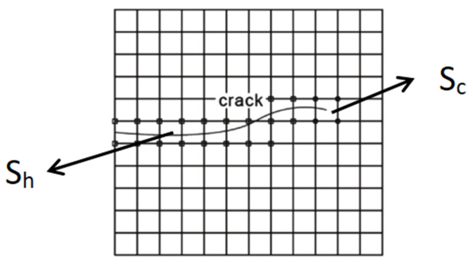
Figure 2.
Multi-scale connection schematic and computational model.
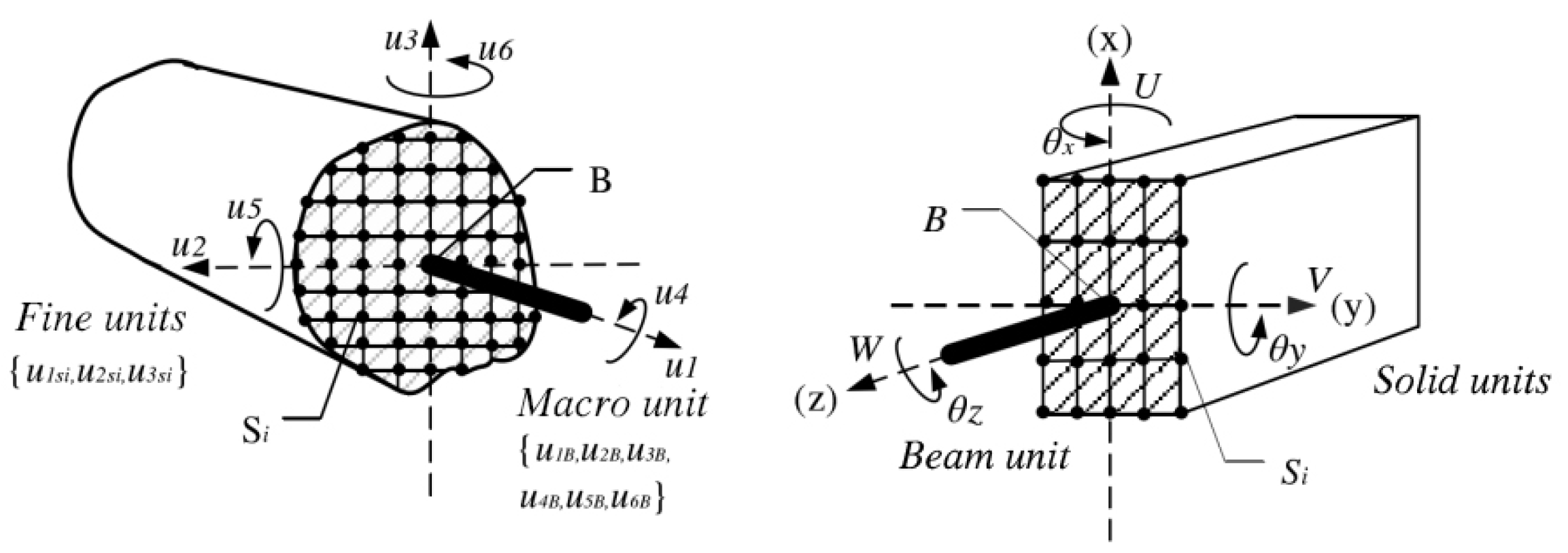
Figure 3.
Q235 steel principal structure model
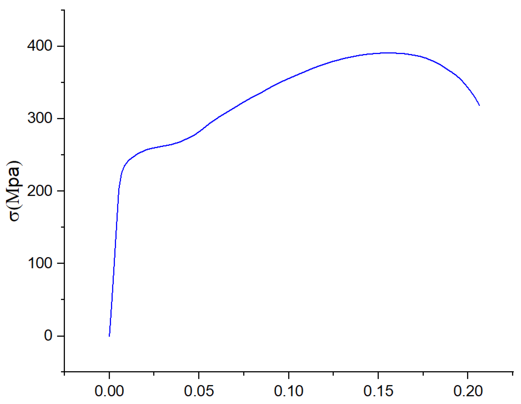
Figure 4.
Schematic diagram of single-sided cracks.

Figure 5.
Schematic diagram of bilateral cracks.
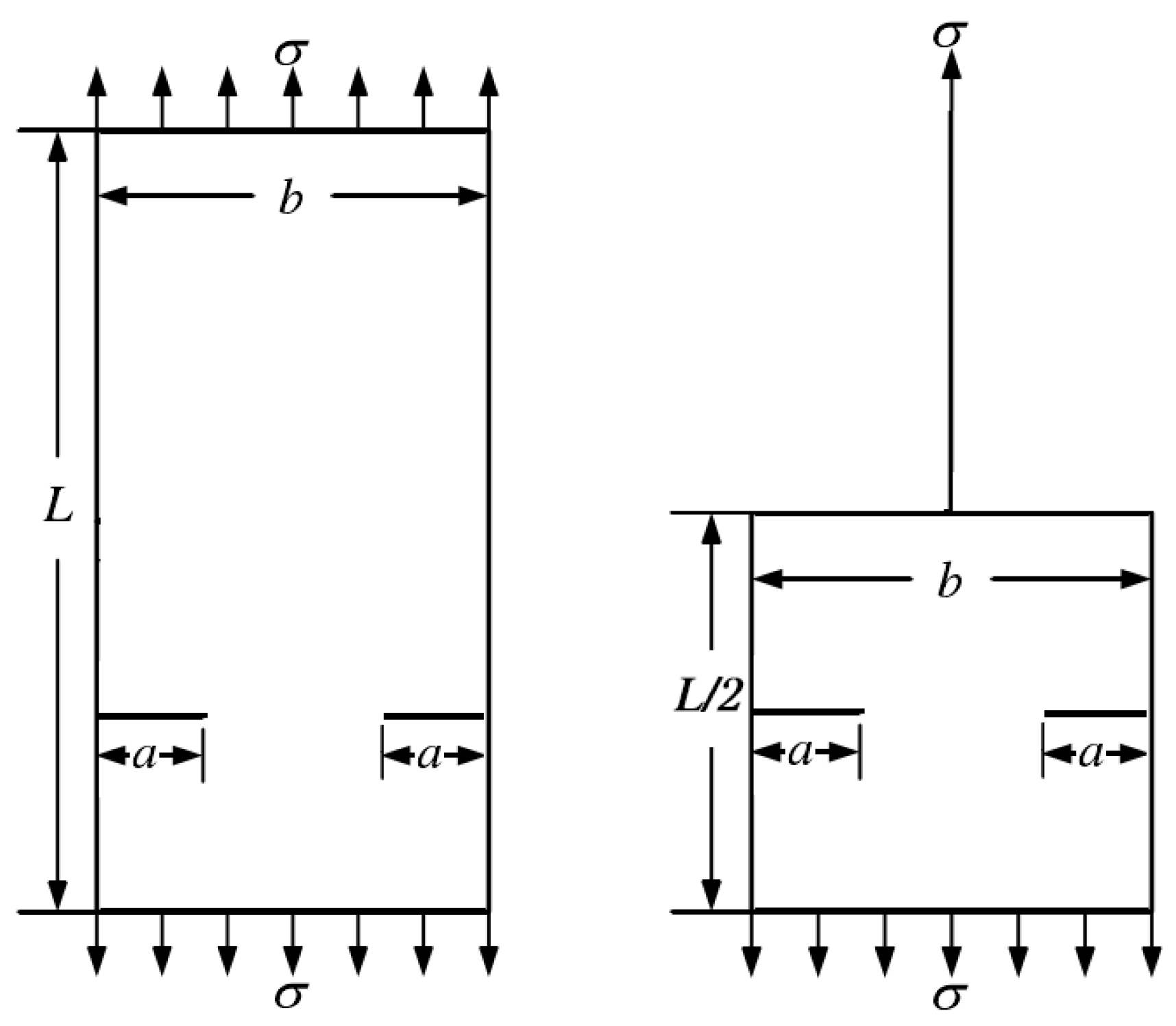
Figure 6.
Diagram of central crack.
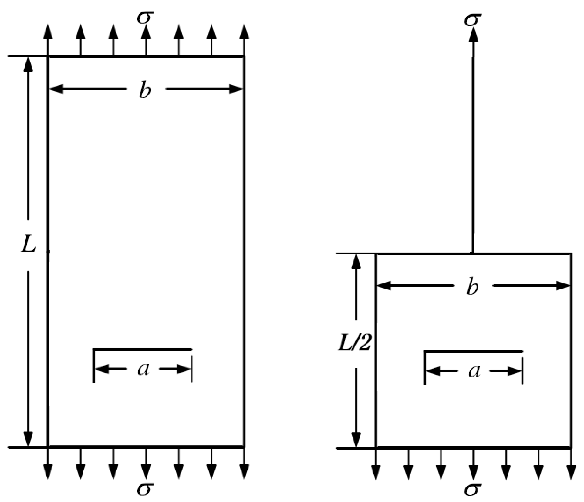
Figure 7.
Diagram of central oblique crack.
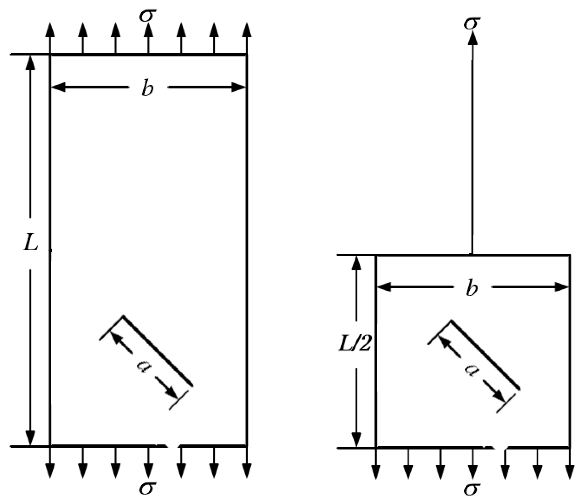
Figure 8.
Loading under the boundary conditions of the working condition.
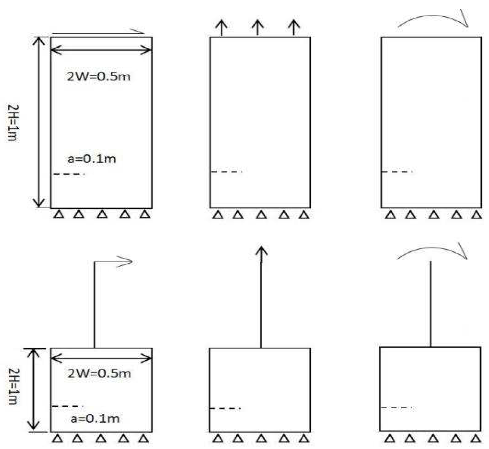
Figure 9.
Meshing of cross-sectional nodes.
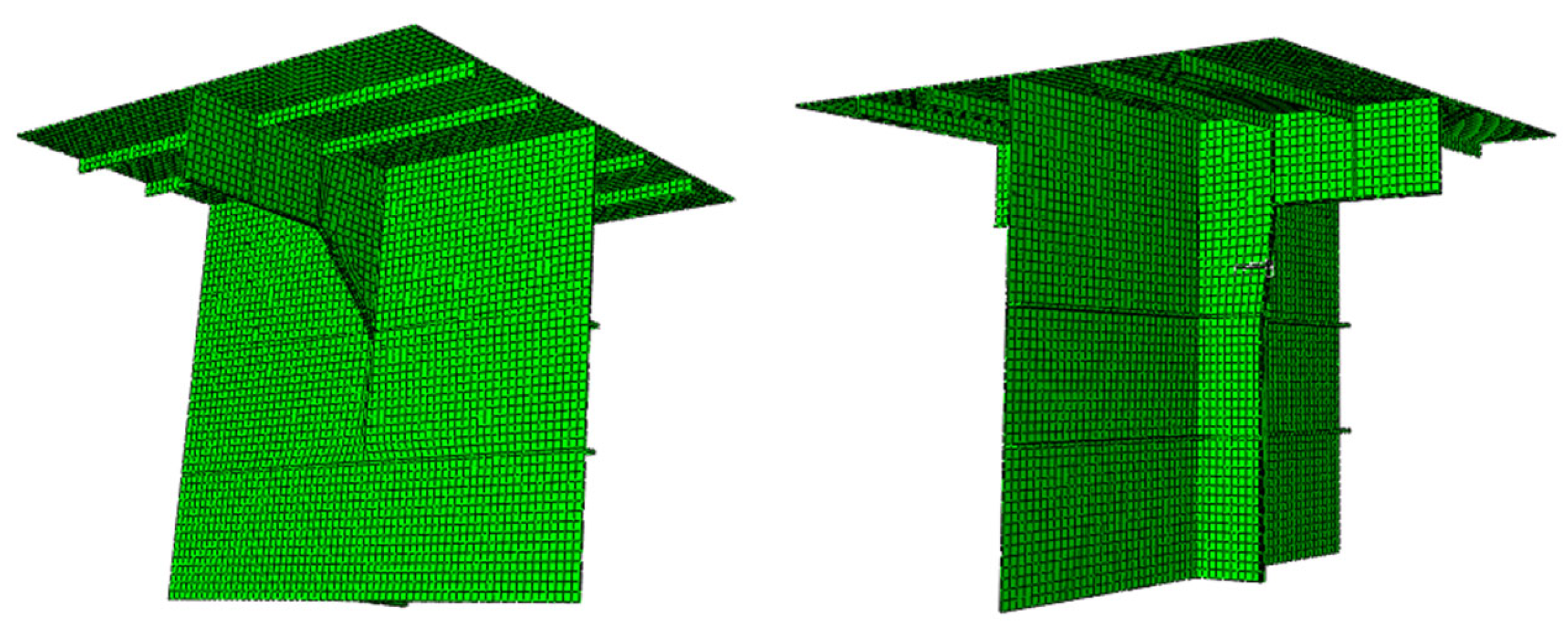
Figure 10.
Single-sided crack stress cloud.
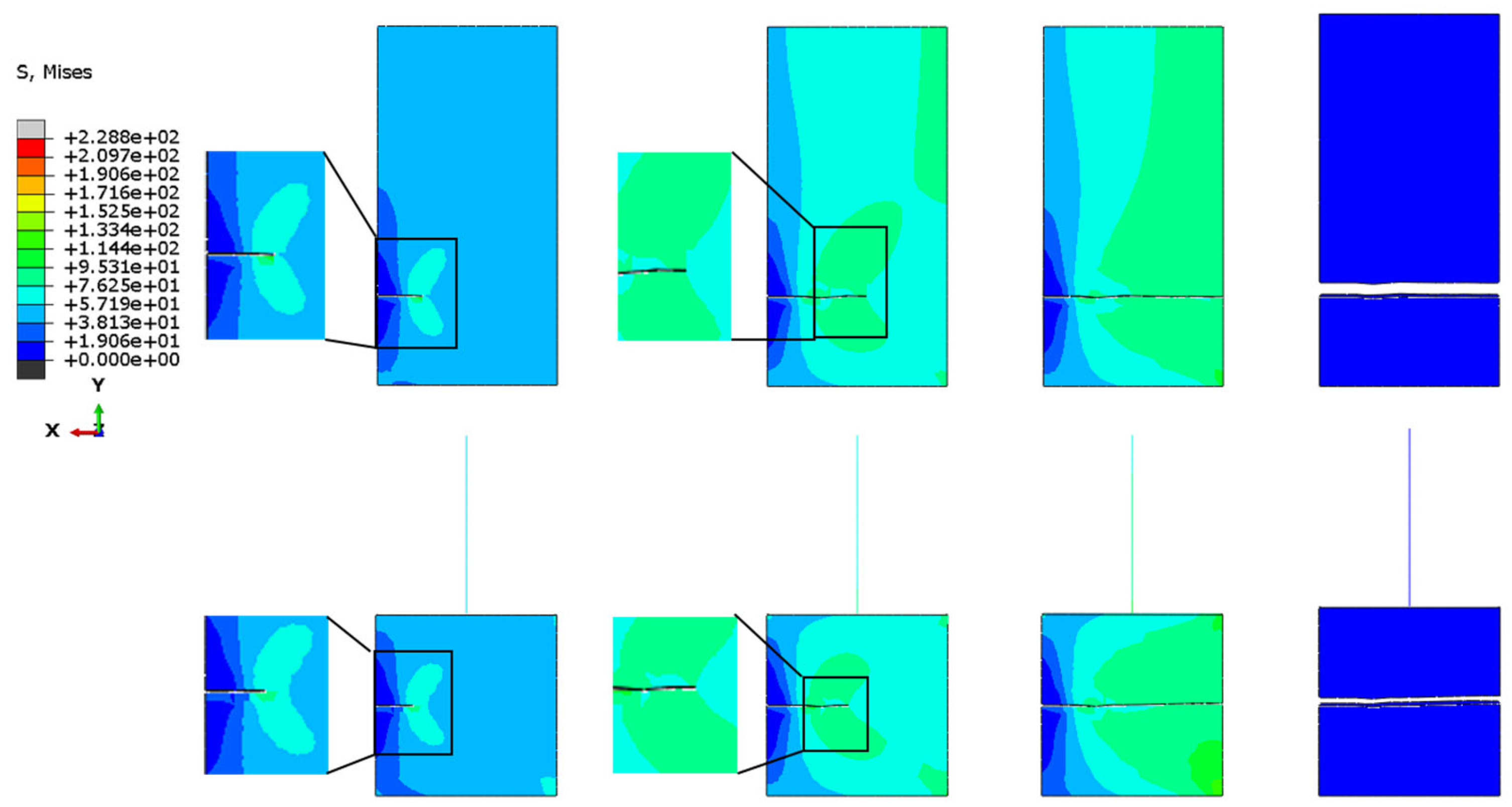
Figure 11.
Bilateral crack stress cloud.
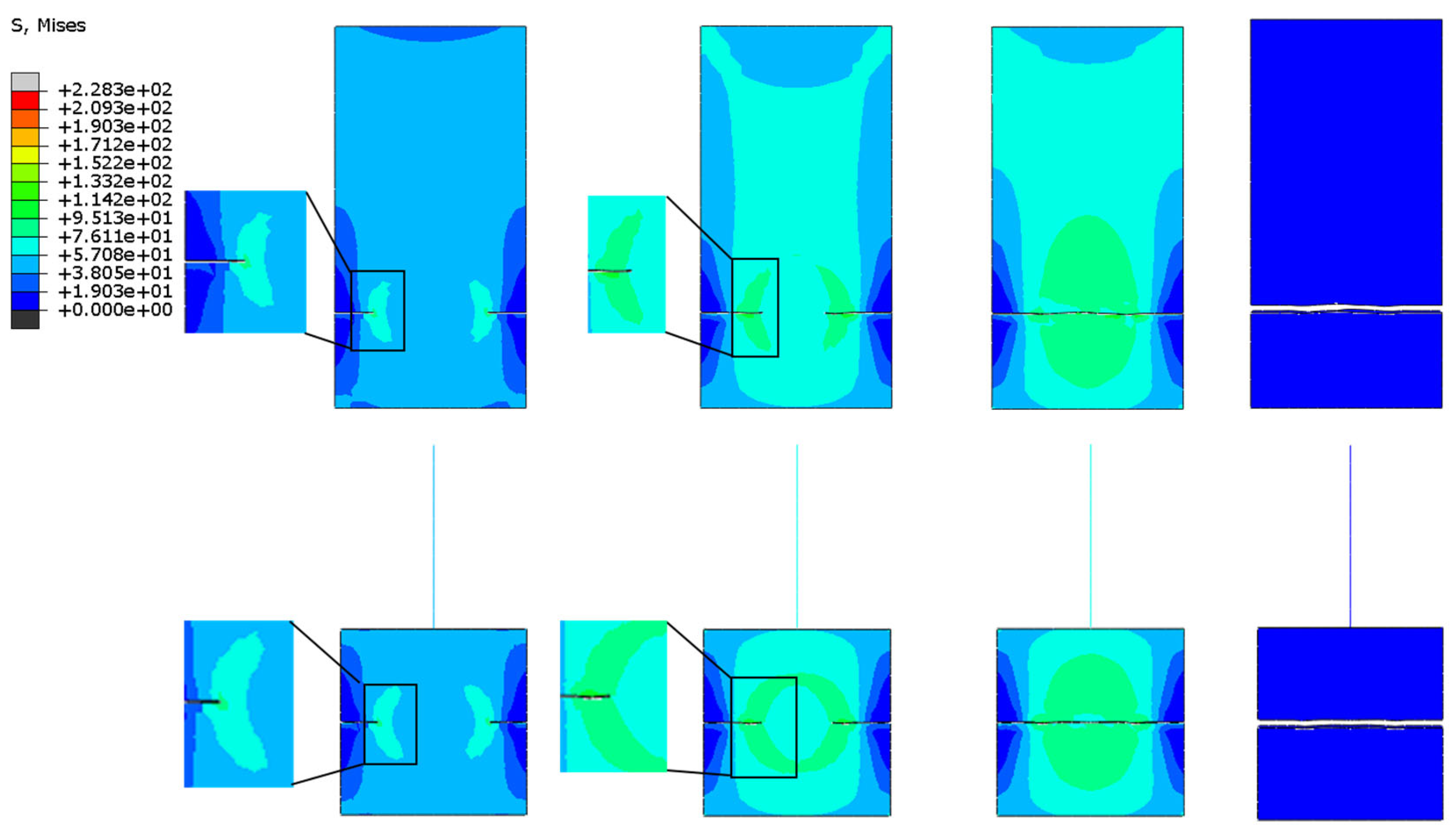
Figure 12.
Central crack stress cloud.
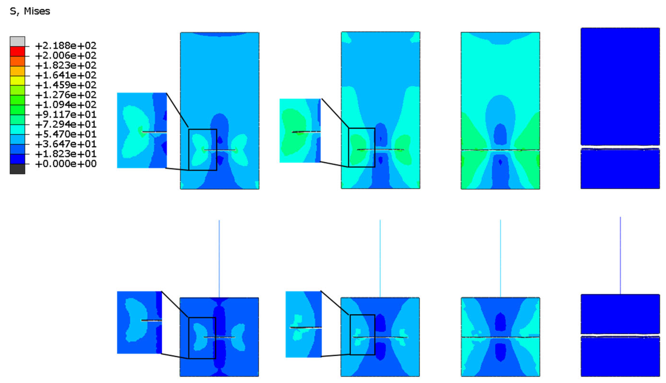
Figure 13.
Central oblique crack stress cloud.
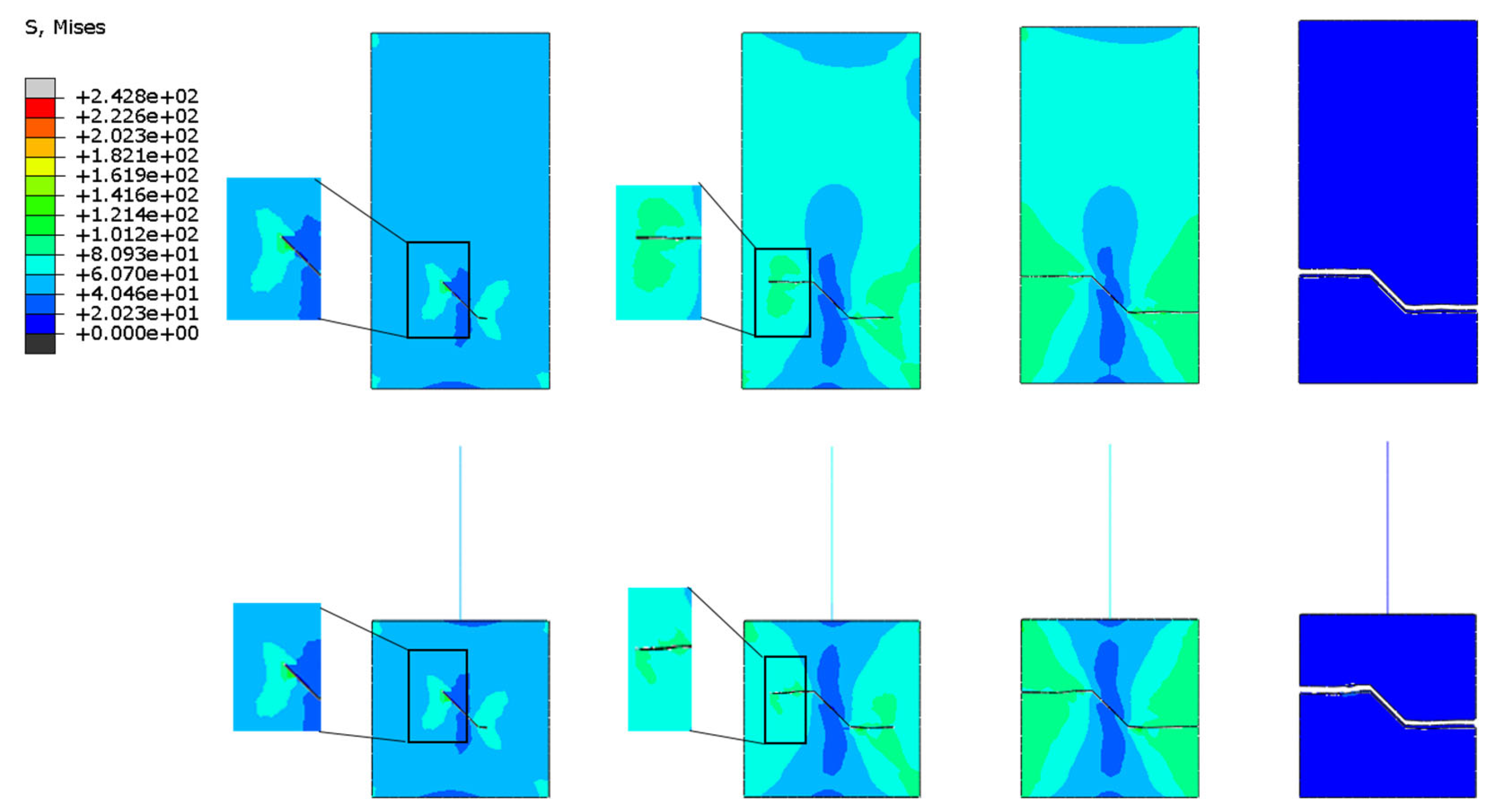
Figure 14.
Comparative analysis of stress intensity factors of different crack types.
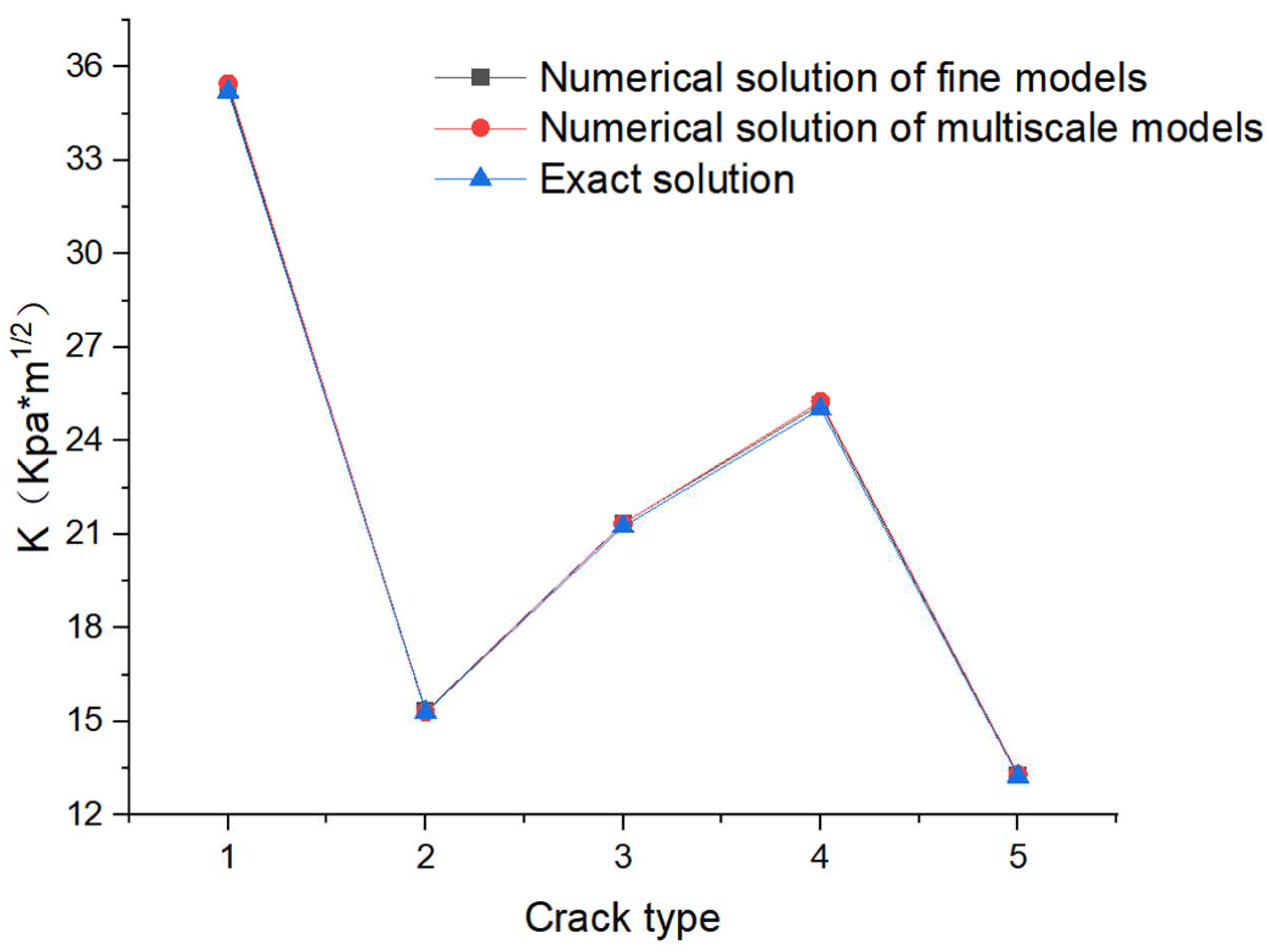
Figure 15.
Comparison chart of working condition 1~4 stress cloud.
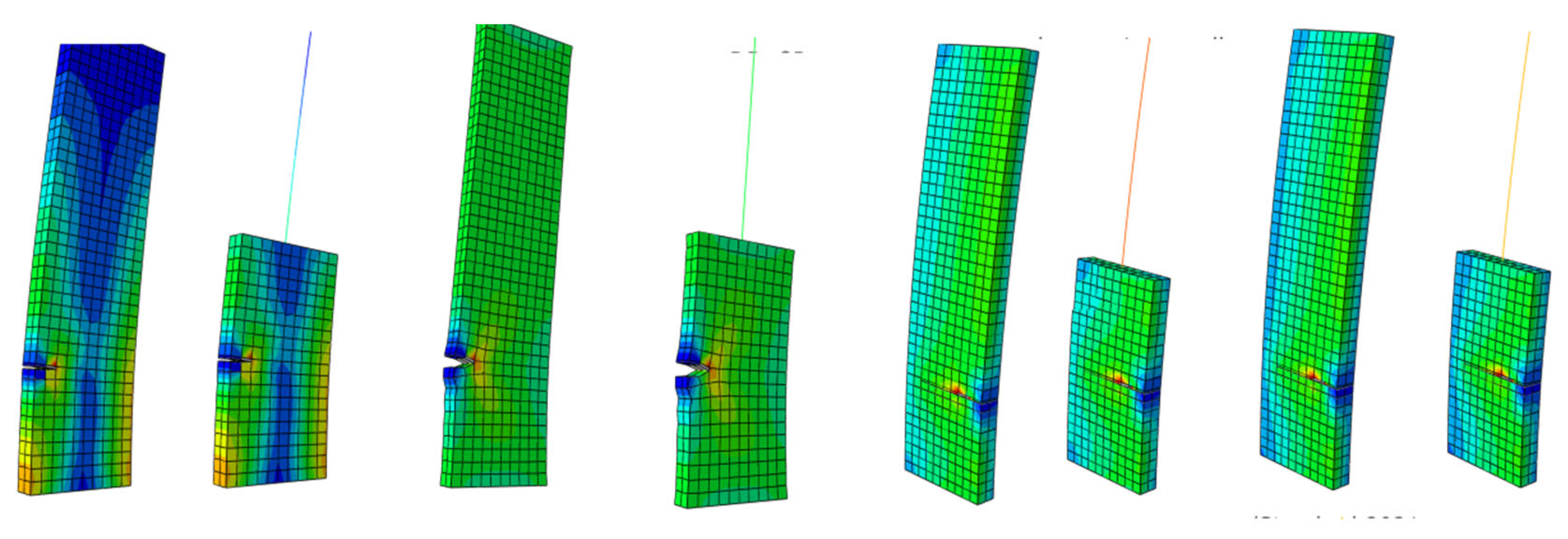
Figure 16.
Trend of stress value change at connection element.
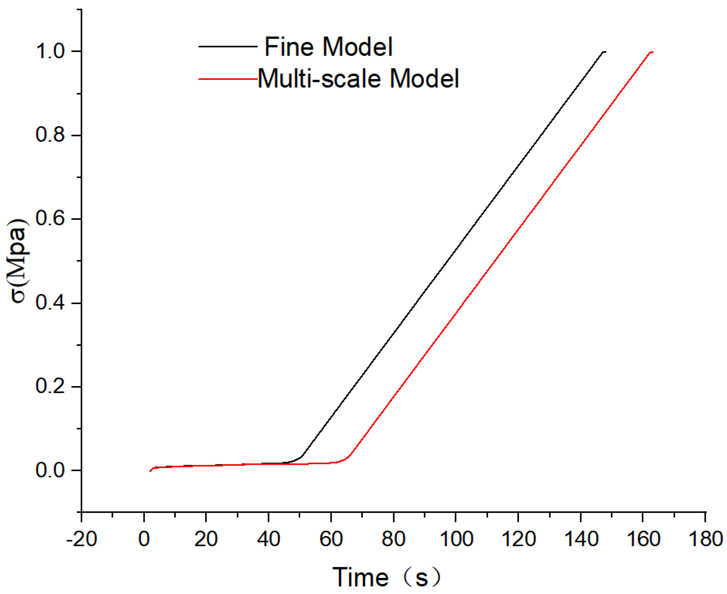
Figure 17.
Mesh encryption analysis of shear working conditions.
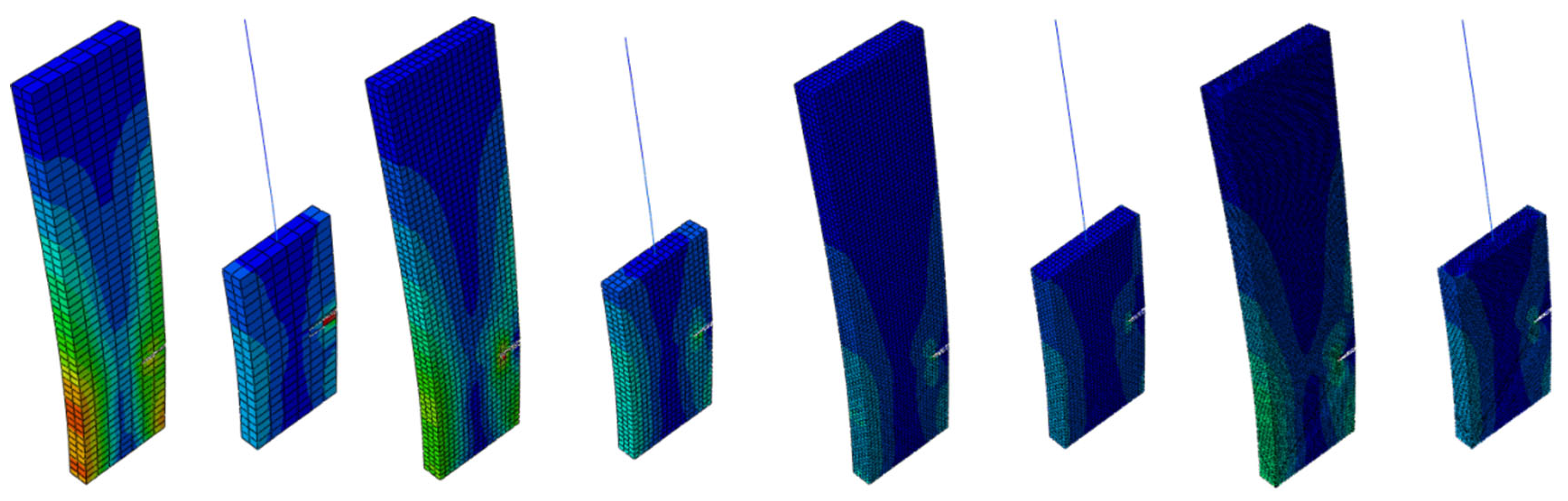
Figure 18.
Comparison chart of node stress cloud.
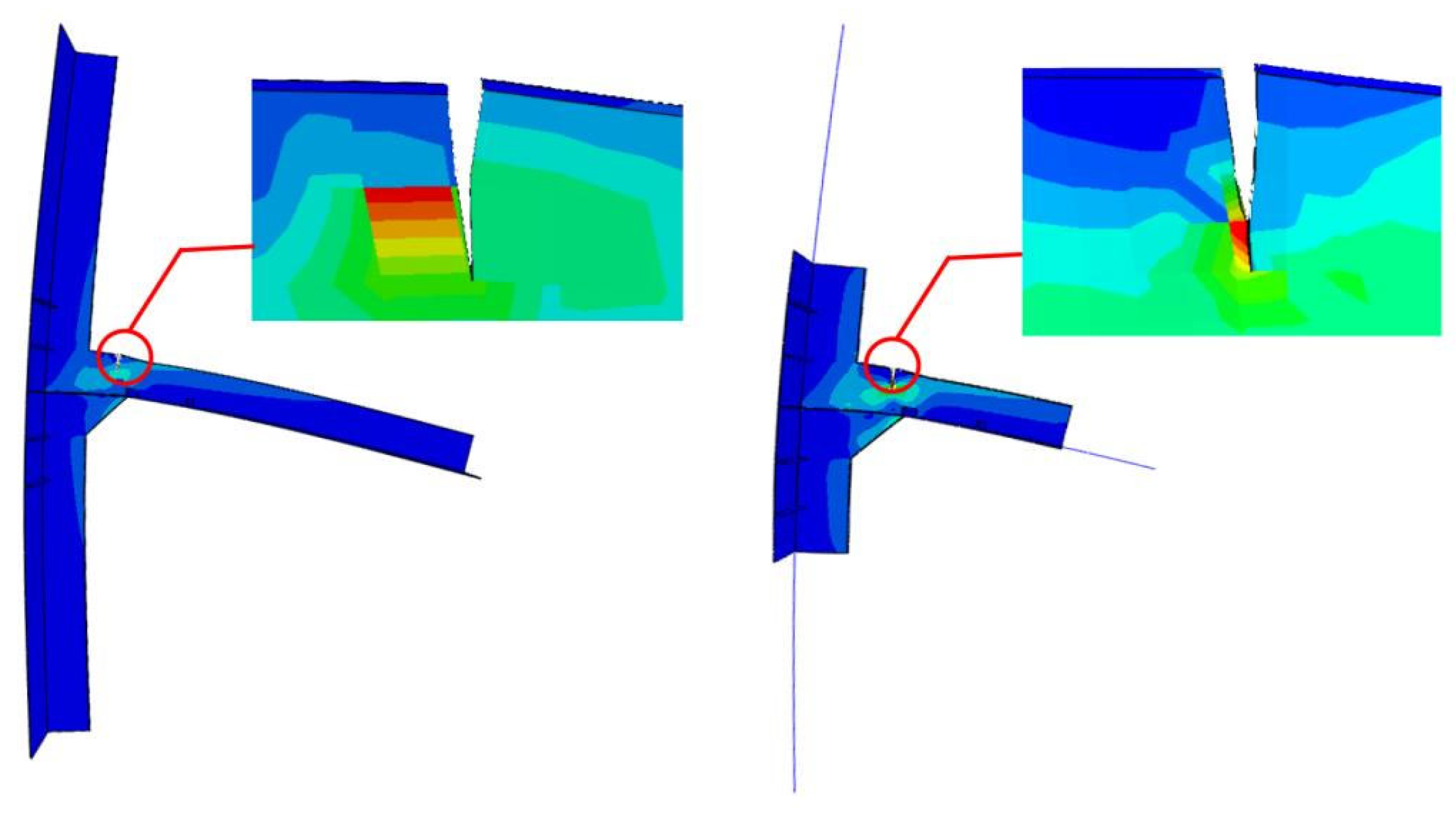
Table 2.
Unilateral cracked rectangular plate material parameters.
| L/mm | b/mm | a/mm | E/GPA | µ | στ/Mpa | σ/Mpa |
|---|---|---|---|---|---|---|
| 40 | 20 | 5 | 206 | 0.3 | 235 | 300 |
Table 3.
Material parameters of bilateral cracked rectangular plates.
| L/mm | b/mm | a/mm | E/GPA | µ | στ/Mpa | σ/Mpa |
|---|---|---|---|---|---|---|
| 40 | 20 | 5 | 206 | 0.3 | 235 | 300 |
Table 4.
Center crack rectangular plate material parameters.
| L/mm | b/mm | a/mm | E/GPA | µ | στ/Mpa | σ/Mpa |
|---|---|---|---|---|---|---|
| 40 | 20 | 5 | 206 | 0.3 | 235 | 300 |
Table 5.
Material parameters of rectangular plate with central oblique crack crack.
| L/mm | b/mm | a/mm | E/GPA | µ | στ/Mpa | σ/Mpa |
|---|---|---|---|---|---|---|
| 40 | 20 | 5 | 206 | 0.3 | 235 | 300 |
Table 1.
Comparative analysis of stress intensity factors for different grid densities.
| The grid occupies the ratio of edge length | Multi-scale model stress intensity factor(Mpa*m1/2) | Fine-model stress intensity factor(Mpa*m1/2) |
|---|---|---|
| 1/2 | 11.6323 | 11.6254 |
| 1/3 | 11.6368 | 11.6264 |
| 1/5 | 11.6265 | 11.6193 |
| 1/10 | 11.6264 | 11.6115 |
Disclaimer/Publisher’s Note: The statements, opinions and data contained in all publications are solely those of the individual author(s) and contributor(s) and not of MDPI and/or the editor(s). MDPI and/or the editor(s) disclaim responsibility for any injury to people or property resulting from any ideas, methods, instructions or products referred to in the content. |
© 2023 by the authors. Licensee MDPI, Basel, Switzerland. This article is an open access article distributed under the terms and conditions of the Creative Commons Attribution (CC BY) license (http://creativecommons.org/licenses/by/4.0/).
Copyright: This open access article is published under a Creative Commons CC BY 4.0 license, which permit the free download, distribution, and reuse, provided that the author and preprint are cited in any reuse.


