
Submitted:
29 December 2025
Posted:
30 December 2025
You are already at the latest version
Abstract
A structure based analysis of the pion’s decay path reveals that neutrinos show up in three flavours, each built up by three identical mass eigenstates. It requires a proper understanding of the nature of charged leptons, such as why the loss of binding energy stops the lepton generation at the tauon level. The analysis reveals fundamental interrelationships between mesons, charged leptons and neutrinos. It is shown that the results of the theoretical model for neutrinos developed in the article are in agreement with the results of the phenomenological PMNS model. The article ends with a discussion on the pros and cons of a structure based theory developed from first principles and phenomenological modelling.
Keywords:
neutrino
; neutrino oscilation
; lepton
; flavour state
; mass state
1. Introduction
The history of neutrinos dates back from 1927 when Wolfgang Pauli formulated a bold hypothesis on their existence that he sighing posited in a letter to Hans Geiger and Lise Meitner [1]. It was the only way out he could imagine to explain the uniformly distributed energy spectrum of electrons that showed up as beta radiation in observations and experiments on radioactivity, such as already since 1914 been noticed by James Chadwick [2]. It was Enrico Fermi, who took Pauli’s hypothesis seriously and who in 1933 developed a theory for beta radiation based on the neutrino existence [3]. In his theory, which presently is regarded as the forerunner of the weak interaction theory, the neutrino is a fermion that eludes observation because of its zero mass and zero charge. Eventually, in 1956, its existence is experimentally confirmed by Reines and Cowan [4].
That experiment marks the start of experimental studies on neutrinos. One of the problems, next to identify suitable physical processes to study the interaction of neutrinos with matter, is the issue how to obtain neutrino fluxes large and strong enough to detect the rare events expected from those processes. Reines and Rowan used a nuclear reactor for the purpose. Their experiment got follow-ups by other ionic neutrino experiments, in particular those based upon knowledge captured in the Standard Solar Model. The idea behind those is, that since the energy of the sun is known and since its major energy production mechanism as well, it is possible to calculate the neutrino flux on earth as well. This flux is defined as the number of neutrinos that, each second pass through 1 m square surface perpendicular to the direction to the sun. This would enable to develop experimental evidence not only in qualitative terms, but in quantitative terms as well.
And it did. Most remarkably, however, those experiments revealed an unexpected result [5]. The predicted neutrino count showed a deficit of about 50%-70% with respect the actually measured count. The solar neutrino problem was born. What happened with the neutrinos emitted by the sun? Why would those not be capable to produce the predicted neutrino count? The inevitable answer to the problem is the awareness that neutrinos are subject to changes when they move from to the sun to the detectors on earth. The most simple approach to this problem is the assumption that neutrinos come in different flavours. Because they are produced in co-production with charged leptons, they show a specific flavour determined by the co-produced charged lepton. This hypothesis could be affirmatively tested by making the neutrino detectors in the experimental equipment no longer exclusively sensitive to electron neutrinos. Nevertheless, a major problem remained: the neutrino flow from the sun is produced from nuclear fusion of Hydrogen atoms into Helium nuclei, thereby producing almost exclusively electron neutrinos. How to explain the change of electron neutrinos into a significant amount of other flavours on their route from sun to earth?
Eventually this tantalizing question has resulted into the bold hypothesis, earlier formulated by Pontecorvo in 1957 - and later adopted as explanation for the missing neutrinos -, that neutrinos are built up by a virtual substructure [6]. Such a virtual substructure would allow neutrino compositions built by three basic eigenstates, different from their flavour states, more or less in the same way as hadrons are composed by quarks. According to this hypothesis, the electron neutrino is in a particular mixture of eigenstates, while a muon neutrino and a tauon neutrino would be in other mixtures. Hypothetically, this would allow oscillations between the flavour states of neutrinos and the loss of coherency would solve the solar neutrino problem.
If substructures are considered as being viable for neutrinos, why would substructures for charged leptons not be viable as well? Why not conceiving the electron, the muon and the tauon as states built by underlying constituents as well? Within the Standard Model the charged leptons are simply considered as elementary particles, and because in the Standard Model everything comes in a three, even a basic question as “why no charged lepton beyond the tauon” has remained unanswered. This article is aimed to show how these issues of the constrained lepton generation and the mass and origin of neutrino’s can be highlighted in the structure based model of particle physics, documented in [7,8]. In the second paragraph of this article it is shown how the structural model for charged and uncharged leptons (neutrinos) evolve from the structural model of mesons as developed in previous work. It is the stepping stone for the explanation of some unrecognized phenomena in the Standard Model of particle physics. The first of these is a proof for the non-understood stop of the lepton generation at the tauon level (paragraph 4). It is shown that this can be traced back to the very same reason as why the quark flavour generation stops at the (ottom) level (topquarks are of a different kind [7,8]). In the fifth paragraph it will be shown why neutrino flavours are composed by eigenstates and how these become manifest as physical mass. The final paragraph contains a discussion on the flavour oscillation phenomenon. Probably the most revealing part of the article is the third paragraph. It shows that the recognition that quarks are non-canonical Dirac particles with two real dipole moments allows an anyonic bond with half-integer spin, thereby revealing one the hand the fundamental correspondence and on the other hand the fundamental difference between mesons and leptons.
2. Structural Models for Pion, Muon and Neutrino
Figure 1 is an illustration of the Structural Model for a pion as developed by the author over the years [8]. It shows that two quarks are structured by a balance of two nuclear forces and two sets of dipoles. The two quarks are described as Dirac particles with two real dipole moments by the virtue of particular gamma matrices. The vertical one is the equivalent of the magnetic dipole moment of an electron. The (real valued) horizontal dipole moment is the real equivalent of the (imaginary valued) electric dipole moment of an electron [9,10].
In a later description, after recognizing that this structure shows properties that match with a Maxwellian description, the quarks have been described as magnetic monopoles in Comay’s Regular Charge Monopole Theory (RCMT) [11]. This allows to give an explanation of the quark’s electric charge by assuming that the quark’s second dipole moments (the horizontal ones) coincide with the magnetic dipole moments of electric kernels . This description allows to conceive the nuclear force as the cradle of baryonic mass (the ground state energy of the created anharmomic oscillator) as well as the cradle of electric charge.
The model allows a pretty accurate calculation of the mass spectrum of mesons. It also allows the development of a structural model of baryons including an accurate calculation of the mass spectrum of baryons as well. This calculation relies upon the recognition that the structure can be modelled as a quantum mechanical anharmonic oscillator. Such anharmonic oscillators are subject to excitation, thereby producing heavier hadrons with larger (constituent) masses of their constituent quarks. The increase of baryonic energy under excitation is accompanied with a loss of binding energy between the quarks. This sets a limit to the maximum constituent mass value of the quarks. It is the reason why quarks heavier than the bottom quark cannot exist and why the topquark has to be interpreted different from being the isospin sister of the bottom quark [8].
Because lepton generations beyond the tauon have not been found, they probably don’t exist for the same reason. In such a picture the charge lepton structure would result from the flip of the antiquark in the pion structure into a quark in a muon structure. This structure is bound together by an equilibrium of the repelling force between the RCMT charges and the attraction force between real scalar dipole moments. In spite of its resemblance with the pion structure, its properties are fundamentally different. Whereas the pion consists of a quark in positive energetic state and a quark in negative energetic state (antiquark) making a boson, the charged lepton consists of two quarks in positive energetic state making a fermion. Figure 3 shows a naive picture of the decay process. In this picture the muon is considered to be a half spin fermion in spite of the appearance of two identical kernels in the same structure. Assigning the fermion state to the structure seems being in conflict with the convention to distinguish the boson state from the fermion state by a naive spin count. Instead, a true boson state for particles in conjunction (instead of a pseudo-boson state shown here) should be based upon the state of the temporal part of the composite wave function. In this particular case, the reversal of the particle state into antiparticle of one of the quarks marks a transformation from the bosonic pion state into the fermionic muon state under conservation of the weak interaction bond.
Under decay, the pion will be split up into a muon and a neutrino. In the rest frame of the muon, the muon will obviously contain the electric kernels and some physical mass. The remaining energy will fly away as a neutrino with kinetic energy and some remaining physical mass. Figure 2 shows the model, in which a structureless neutrino is shown next to a muon with a hypothetical substructure.
Let us proceed from the observation that there is no compelling reason why the weak interaction mechanism between a particle and an antiparticle kernel would not hold for two subparticle kernels. In such model, the structure for the charged lepton is similar to the pion one. It can therefore be described by a similar analytical model. Hence, conceiving the muon as a structure in which a kernel couples to the field of another kernel with the generic quantum mechanical coupling factor , the muon can be modeled as a one-body equivalent of a two-body oscillator, described by the equation for its wave function ,
In which is Planck’s reduced constant, 2 the kernel spacing, is the effective mass of the center, its potential energy, and the generic energy constant, which is subject to quantization. By convention the coupling factor has been defined as the square root of the electromagnetic fine structure constant as The potential energy can be derived from a potential . Similarly as in the case of the pion quarks, this potential is a measure for the energetic properties of the kernels. It characterized by a strength (in units of energy) and a range (in units of length: the dimension of is [m-1]).
The potential of a pion quark has been determined as,
These quantities have more than a symbolic meaning, because in the structural model for particle physics developed so far [7,8], has been quantified by , in which (126 GeV) is the energy of the Higgs particle as the carrier of the energetic background field. An equal expression for the potential would make the muon model to a Chinese copy of the pion model.
Instead the potential of the muon kernels is described as,
The rationale for this modification is twofold. In the structural model for the pion, the exponential decay is due to the shielding effect of an energetic background field. If the muon is a true electromagnetic particle, there is no reason why its potential field would be shielded. This explains the origin of the neutrino as an additional energetic particle required to compensate for the difference between the shielded and the unshielded potential. That the gyrometric factor of the muon (not be confused with the quantum mechanical coupling factor ) is different from pion’s one is a consequence from the shielding issue [8]. Considering that the potential is a measure of energy, and that the break-up of a pion into a muon and a neutrino takes place under conservation of energy, it is fair to conclude that the neutrino can be described in terms of a potential function as well, such that
We may even go a step further by supposing that similarly as the muon, the neutrino can be modelled by a composition of two kernels. If so, each of these neutrino kernels have a potential function , such that
It is instructive to emphasize that the potential function of a particle, be it a quark, a charged lepton or a neutrino, does not contain any information about its mass. In that respect it is not different from the potential function of a charged particle like an electron. Furthermore it is of interest to emphasize that, like mentioned before, the quantities and have a physical meaning in quantitative terms.
The muon is not a stable particle. It may lose its weak interaction bond under decay into electrons. Figure 3 shows an interpretation of the process. It shows how the weak interaction boson that binds the pion quarks disintegrates into the muon and the muon neutrino and how the two may recoil into a weak interaction boson that decays into an electron and electron antineutrino. This picture and the description just given evoke two basic questions.
The first one is this. If it is true indeed that the behaviour of the pion can be modelled as an anharmonic oscillator, why would the muon not be subject to a similar excitation mechanism as shown by the pion? The answer is that the muon is subject to excitation indeed, thereby producing the tauon state. Actually, this has been documented in previous work [12]. But, unlike as in the case of pions, it is a single stop. This excitation mechanism will be summarized in the next paragraph. It will be shown that this analysis will give a firm support to the model captured by the equations (2-7).
The second issue is the question how the muon decays into an electron and a neutrino. In principle this process is a statistical one, in principle not different from the way as originally proposed by Fermi [3,13].
Figure 3.
A charged pion decays into a charged lepton (muon) and its associated neutrino because of emission of the vector weak interaction boson. Subsequently, the muon and the neutrino recoils into a weak interaction boson that subsequently decays by a statistical process into an electron and an antineutrino.
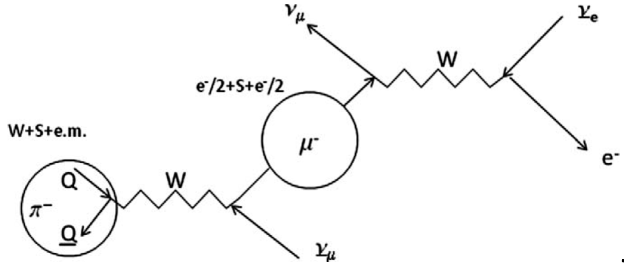
This paragraph is now concluded with the statement that the leptons show up in three generations of charged-uncharged twins. In the remainder of this article it will be shown that the muon twin is the result of the pion’s loss of its bond with energetic background field . It can be analyzed from first principles. The tauon twin is an excitation. The analysis of the electron twin is problematic, because, unlike the muon, the electron cannot be modelled by an internal structure. What can be done, though, is conceiving the muon twin as a relativistic state of the electron twin. Such view makes sense, because the muon twin is the pion, which is nothing else but the non-relativistic state of the weak interaction boson.
3. The Charged Lepton as an Anionic Bond Between Quark-Type Dirac Particles
In principle, the structural model shown in figure doesn’t hold only for a quark and an antiquark in conjunction, but it may hold for two quarks in conjunction as well. In the case that the quark are normal spin 1/2 fermions, such a diquark, similarly as the quark and the antiquark junction, will have integer spin. Hence a property that is usually associated with a boson. However, such a boson cannot have force-transmitting properties, because such property requires an overall wave function with a real temporal part next to its real spatial part, like, for instance shown by photons. It means that the nomenclature “boson” is subject to convention. In the Standard Model the boson is identified with statistics (Bose-Einstein vs. Fermi-Dirac), in the Structural Model [8], the boson is identified with its wave function.
The muon model proposed in paragraph 2 is a two-quark junction. Clearly, the muon is not a force-transmitting particle. But neither it can’t be a Standard Model boson, because the muon is a fermion with spin 1/2. Nevertheless, as to be shown in the next paragraph, the modelling of the muon as a two-body harmonic oscillator is extremely fruitful. It gives a predictable value for the mass of the tauon, it explains why no charged lepton can exist beyond the tauon and it predicts three mass eigen states for the neutrinos. Not discussed in detail in this article, but shown in [8], is the proof that the mass of the muon (105 MeV) can be calculated by first principles from the rest mass of the pion (about 140 MeV). A result that in the Standard Model has to be accepted as an empirical fact only. How to escape from the spin paradox?
The solution of the paradox is the recognition that the muon type bond between two quarks in particle state is an anyonic bond. In such a bond a particle cannot rotate around the static position of the other particle under maintenance of the properties [14]. This makes the bond fundamentally different from a “bosonic” diquark bond such as a Cooper pair or the highly unstable potential bond between two electrons kept in equilibrium by a balance between the repulsive electric force and the attraction force of their properly oriented magnetic dipole moments [15]. It has been recognized for long that the statistical properties of the anyonic bond are different from the “bosonic” bond. The anyonic bond allows a half integer spin state for the junction, while the “bosonic” bond is in integer spin state. It will be clear that the identification of quarks as Dirac particles with two real dipole moments allows to recognize charged leptons, such as the muon as the anyonic bond between two quarks.
4. The Pion and the Muon
The 006Dodeling of the pion and the muon by anharmonic oscillators captured in the mathematical description shown by (2-4) does not contain any particular quantum mechanical property. A binomial expansion of the potential energy allows to rewrite the wave equation as,
The quantum wave equation can be normalised to the simple form by
in which , ,
The oscillator settles into a minimum energy state at . At this setting we have
Using the potential function (3), a little algebra reveals the simple relationships,
(note: as to be memorized later, these expressions are different for the pion oscillator.)
Figure 5 shows the potential (energy) of the muon’s center of mass, defined by (1) and (7) as a function of its deviation from the spatial center. Each curve in the figure is characterized by a particular parameter value for the (normalized) spacing between the poles. There is a clear minimum for , an increase of the curvature for and a decrease of the curvature for . If the two poles are spaced in the state of minimum potential (), the vibration energy of the muon is in the ground state. As long as the curves show a minimum with a negative value, the configuration shows an amount of stability-preserving binding energy. It will be clear that the binding energy is lost for narrow spacing. In figure 5 it is illustrated that the energy constant level of first excitation in ground state may correspond with the ground state energy constant of the configuration at a smaller spacing.
This is the reason why, under excitation conditions, the configuration may jump from the muon state to the tauon state. It will be clear that the jump to the level of second excitation cannot be made under preservation of negative binding energy. Hence, charged leptons beyond the tauon particle are non-existing.
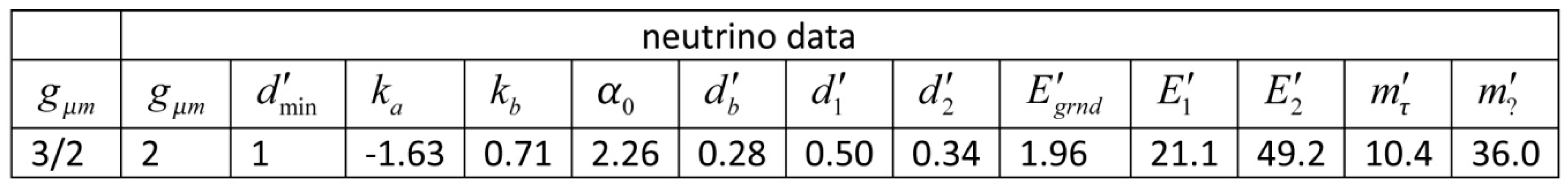
A detailed analysis of the anharmonic oscillator can be found in [7,8]. The table shown in figure 6 summarizes the relevant data and results.

Table 1.
Explicit expressions for the parameter values of the muon oscillator and the pion oscillator.
Table 1.
Explicit expressions for the parameter values of the muon oscillator and the pion oscillator.
| Property | Parameter | Muon | Pion |
|---|---|---|---|
| quantum mechanical coupling factor | |||
| gyrometric ratio | |||
| normalizing spacing parameter | |||
| spacing for minimum energy | |||
| constant term potential energy | |||
| quadratic term potential energy | |||
| oscillator constant | |||
| mass relationship | |||
| mass curve |
In both oscillator models the spatial dimensions are normalized such that the spacing between the quarks in the state of minimum energy . As noted before, the normalizing spatial parameter is closely related with the energy of the Higgs boson as . This normalization gives different gyrometric values for the muon oscillator and the pion oscillator. The normalization gives for the muon and pion in the normalized potential energy different values for and . The parameter is a subtle and important one. It relates the pion oscillator frequency with the weak interaction boson . Because the pion decays under emission of the weak interaction boson, it is tempting to believe that its equals . Actually this is not necessarily true, because in fact, the weak interaction boson energy is the sum of the binding energy and the ground state of the pion oscillator: the frequency can be higher and the binding energy lower. It is a subtlety as a consequence from the anharmonic behavior of the oscillator, not explicitly identified by me before in some of my previous papers). Eventually, this energy settles as the rest mass energy in the rest frame of the pion. It makes the weak boson (GeV) to the relativistic state of the ( MeV) rest mass of the pion flying at near light speed. A careful analysis allows the calculation of a relationship for as shown in the table. The muon oscillator, though, although anharmonic as well, shows a more regular behavior. It shows equal shares of energy in binding energy and ground state energy. Hence, its energy equals the boson . All this allows to calculate, from the Structural Model’s first principles, the rest mass of the muon (105 MeV) from the pion’s rest mass (140 MeV) as reference, while such analytical relationship cannot be established in the Standard Model , in which it is left as an empirical fact.
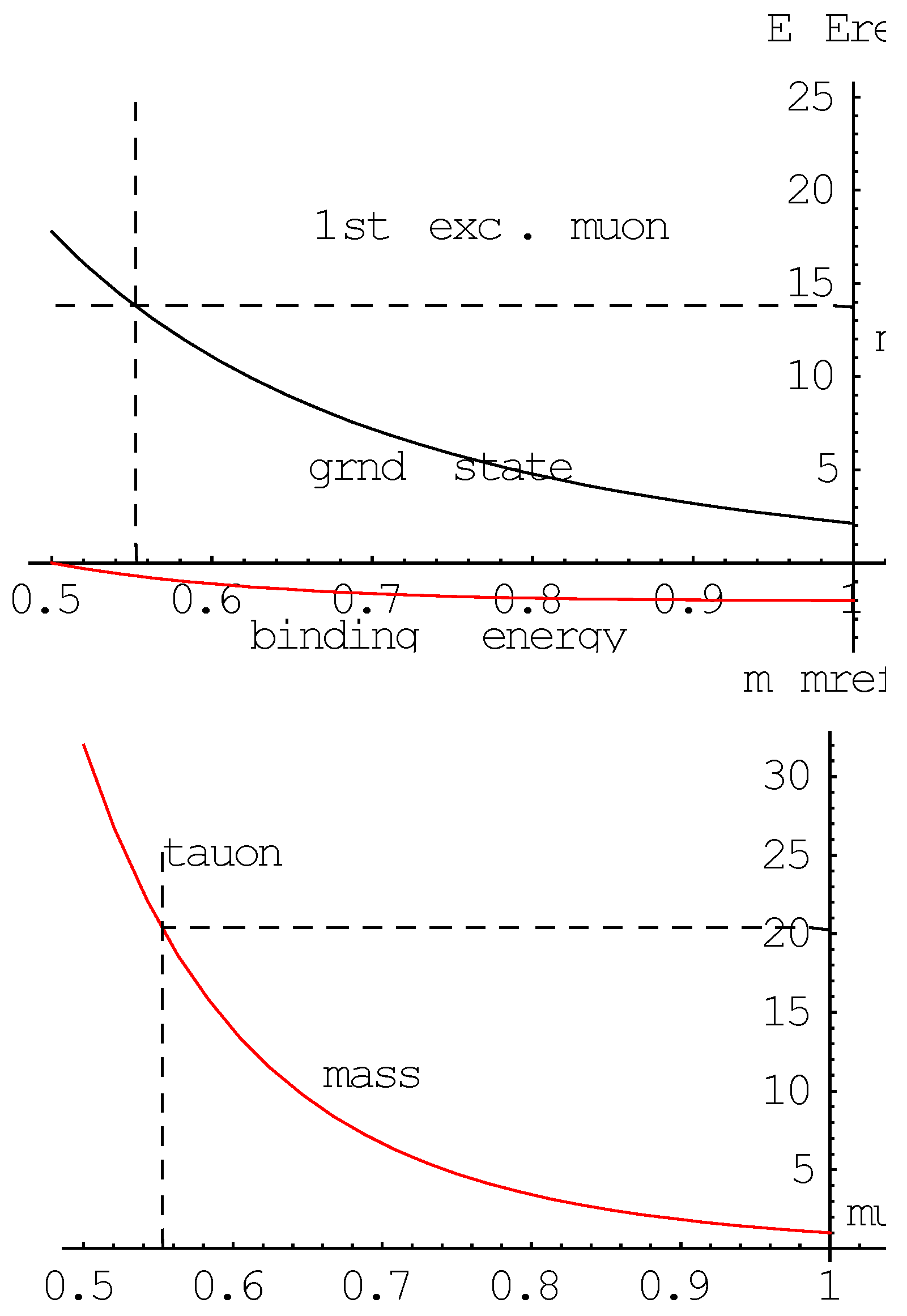
The normalized wave equation allows to calculate by simple computer code the ground state energy as a function of the spacing . This is shown in the upper part of figure 6. It also allows to calculate the excitation levels. The dashed line in that part shows the level of first excitation. It may seem as if the energy level of the first excitation is far beyond reasonable physical expectation, because an ideal harmonic oscillator would show at first excitation only three times the ground state value In that respect the picture is somewhat misleading. One should, however, take into consideration that both these values must be established from the bottom level, determined by the binding energy. In this picture the binding energy level in relative amounts is -2, the ground state energy is 2 and the first excitation level is 13.8. This makes the excitation to ground state ratio about 13.8/4 = 3.80. The difference with the factor 3 of the ideal harmonic oscillator shows the effectiveness of the computer code, in which the anharmonic nature of the oscillator is taken into account.
The lower part of figure 6 shows that, at spacing 0.55, the relative mass value of the structure amounts to 20.3, a value that is predicted by the mass law shown at the bottom line of the Table. This means that the tau particle’s mass is expected being 20.3 times larger than the muon’s mass, which, although satisfying in terms of order of magnitude, does not fit nicely to the PDG data book value of about 1.78 GeV/c2. The difference is due to an overestimation of the value. It can be explained by recognizing that this value has been determined from a truncation in the series expansion of shown in (7). In [8] it is shown that replacing the truncated value by the approximated value gives the required correction. The red curve in the upper part is the binding energy curve. At the quark spacing 0.55, the binding energy still is (slightly) negative. The picture makes clear that excitation beyond tauon level cannot result in a stable lepton configuration. Hence, no charged leptons are found next to the muon and the tauon.
Figure 6.
The lower curve shows the dependence of the lepton’s physical mass on the pole spacing. The upper graph shows that the pole spacing of the tau particle is determined by the equilaty in vibration energy of the muon’s first excitation level and the ground state vibration energy of the heavier tau particle. Note that the binding energy of the tau particle is just slightly negative.
It is worthwhile to note that the excitation mechanism of leptons is somewhat different from that of the mesons. This is due to the fact that the lepton structure does not allow an asymmetry between the kernels. While in the lepton structure the two kernels both have the same values for and , although different for the muon case and the tauon case, the meson excitation mechanism allows asymmetric structures, with different values for and for quarks in the same structure.
5. The Neutrinos and Their Mass States
The analysis of the muon neutrino is not very different from that shown for the charged lepton. The only difference is that the potential function of the quark (2) is replaced by the potential function of the neutrino kernel (5). Figure 7 shows a graphical representation of the behavior of the neutrino. Note that the neutrino has two additional stable quantum states within the range determined by the binding energy. The behavior of the neutrino is captured by the data shown in Figure 8.
It is tempting to interpret the quantum states of neutrinos in a similar way as in the cases of pions and muons. It would mean that the muon neutrino would be in the ground state of the muon neutrino oscillator and that it first excitation would produce the tauon neutrino. But if so, what kind of neutrino would be produced at the (stable) second level of excitation? And what about the electron neutrino?
In the neutrino case, however, there is a good reason for a different interpretation. It can be understood if the origin of the neutrinos is considered once more. Accepting the model formalized by equation (5), one may expect that it will not only hold for the origin of muon neutrinos from the decay of pions into muons, but that it also holds for the origin of the tauon neutrino by a decay of a meson into a tauon. Such a process is shown by a decay mode of the charmed meson [16],
Because the charmed meson is a scaled version of the pion and the tauon is a scaled version of the muon, the only difference between the wave function of a tauon neutrino and a muon neutrino is in the constant in eq. (5). It means that the tauon neutrino is subject to the same excitation mechanism as the muon neutrino. In normalized representation it shows the same eigenstates. The difference in makes the tauon neutrino more energetic, but not necessarily in terms of rest mass. In fact, the excitation mechanism discussed so far, allows two related, but different, interpretations. For hadrons and charged leptons we have conceived excitation as an increase of rest mass in rest frame, while equivalently excitation can be explained as conserved rest mass at an increase of speed. As to be elaborated further in this text, the latter explanation holds for neutrinos.
The electron neutrino would have a natural fit in this view. The caveat, though, is that, while the we have a clear picture for the structural composition for the muon, tauon and their neutrinos, it is less clear for the electron and electron neutrino. Nevertheless, their origin is clear. Next to the muon decay, it is a product of neutron-proton decay. The solar neutrino produced from the fusion of Hydrogen nucleons to the Helium kernel. So, for reasons of symmetry, let us accept the electron and its neutrino as the third doublet in the lepton hierarchy akin to the other two.
6. Neutrino Oscillations
In such interpretation there would be three flavor components, i.e. an electron neutrino, a muon neutrino and a tauon neutrino, respectively, with wave functions , , and three basic wave components . such that
in which is a 3 x 3 unitary matrix. The components of it can be conceived as amplitudes of three basic wave functions , such that we have a system of three simultaneous linear equations for the amplitudes of three constituting basic wave functions.
Observations by huge impressive modern neutrino detectors [20,21] show that neutrinos in their free flight may change their flavours in an oscillating mode. The oscillation process is a continuous trade-off between mass and speed in the basic neutrino wave packets, which, on the long run, eventually decoherences the initial distribution of the flavours into an equal distribution. Adequate descriptions of this process can be found in textbooks and tutorials. Up to now no key is available to assess the rest mass of the neutrinos.
What has been achieved, though, is the assessment of numerical values for the squared mass differences and of the basic wave function objects.
It is at this point where the anharmonic oscillator model of the neutrino is highly relevant. The experimentally assessed numerical values for these mass differences are
Supposing that the mass eigenstates of the neutrinos are related with the eigenstates in the neutrino model derived in the Structural Model (shown in the preceding paragraph), these mass eigenstates must correspond with the ground states in that model. But if it is true indeed that the model applies to states of energy for neutrino rest masses at different propagation speeds there must be some parameter that distinguishes the tauon neutrino from the muon neutrino. We know now from the Structural Model that fermions in excited state have a narrower spacing between the kernels of the anharmonic oscillator model than in the ground state. Inspection of the table shown in figure 8 shows that, whereas this spacing in ground state is at , the spacing in excited state is at . This difference has an influence on the binding energy of the particle. The smaller the spacing, the lower the binding energy. Referencing to the excitation model of the neutrino discussed in the previous paragraph, it implies that the binding energy of the muon neutrino is larger than the binding energy of the tauon neutrino, while their rest masses are the same. Let us make this explicit by equations.
Generically, the binding energy is given by [8],
Because the binding energy via is a reference parameter in the mass formula of the muon, we have, denoting the mass state of the tauon neutrino as and that of the muon neutrino as
Hence, from (12),
This allows to calculate the mass eigenstates in quite accurate relative precision and in rather accurate precision as well. The computer code of the anharmonic oscillator modelled by (5) gives
from which, under consideration of (12) and can be calculated as,
7. Prediction and Verification
Now that we have shown that the Structural Model of particle physics allows us to calculate the three mass eigenstates of neutrinos we are faced with the question if this calculation has to be considered as prediction or as proof. Obviously, the most convincing verification is an experimental proof. But these masses are so tiny that it questionable whether a definite experimental proof of this result would ever be possible. Nevertheless, a substantial support would be obtained if the electron can be included into the framework. If so, a second independent route would be at hand to verify the prediction. It is a subject of further research.
Note that the prediction not only involves the assessment of numerical values for the mass eigenstates, but that it includes the conclusion as well that normal ordering of these eigenstates is the correct one.
8. Discussion
In this article a theory for neutrinos has been presented that shows a natural fit with a structural view on particle physics. It has been shown that, if the origin of the charged leptons is understood first, the origin of neutrinos can be understood from first principles. It has been shown that charged leptons and mesons have a common origin. The archetype meson, i.e. the pion, is a bond between a quark and an antiquark. The structural view on particle physics allows to describe this bond as a quantum mechanical two-body anharmonic oscillator. The justification of this description relies upon the awareness of a Dirac particle mode that shows two real anomalous dipole moments [9,10]. It makes the quark, as Dirac mode particle, different from an electron-type Dirac particle. The latter one shows an imaginary anomalous dipole moments next to a real one. The archetype charged lepton is the muon. Whereas the pion is a bond between a quark and an antiquark, the muon is a bond between two quarks in particle state. Owing to the anyonic nature of this bond, the muon shows non-integer spin. Similarly as the pion, it can be analyzed as a quantum mechanical two-body anharmonic oscillator. It predicts the mass of the tauon and the stop of the charged lepton generation beyond the tauon.
Considering the origin of the muon neutrino next to the muon as the decay product of the pion allows the derivation of an analytical description for the muon neutrino. This description reveals three mass eigenstates for the muon neutrino. It has been shown in the article that the same eigenstates are shown by the tauon neutrino that originates in a decay mode of the charmed meson Ds. So far, the inclusion of the electron neutrino in this theoretical framework is only based on a phenomenological fit, because, unlike the muon-tauon relationship, a theoretical electron-muon relationship is still to be found. It is one of two theoretical challenges left. The other one is the challenge to find a theoretical explanation for the quantitative distribution of the mass eigenstate shares in the neutrino flavours.
In spite of the two challenges left, it is fair to conclude that the theoretical concept for neutrinos developed in this article is not in conflict with the present PMNS theory. The PMNS theory is a stand-alone phenomenological theory. It is based upon a heuristic model with unknown parameters. It is followed by a set of observations to make the unknown parameters to known values. After that results of new experiments are predicted. If the actual results of these experiments are in agreement with the predicted ones, it is said that the theory is correct. This is the standard philosophy in modern physics — and a powerful one, because the fitting with experimental data makes the theory accurate an precise. More precisely often than a theory derived from first principles. So far, attempts have failed to connect the PMNS theory with the canonical Standard Model of particles, which, by the way, is phenomenological to great extent as well. The lack of this connection is a reason to believe that a neutrino concept will help to conceive a theory of “New Physics”. The theoretical model developed in this article shows a natural fit in a structural view on particle physics. It is a possible stepping stone to further insights.
References
- https://www.radioactivity.eu.com/site/pages/Neutrino_Hypothesis.htm.
- Chadwick, J. Intensitatsverteilungimmagnetischenspektrum der beta-strahlen von radium B+C. Verh.DeutschenPhysik.Gesellschaft 1914, 16, 383. [Google Scholar]
- Fermi, E. Versucheiner Theorie der β-Strahlen. ZeitschriftfürPhysik 1934, 88, 161. [Google Scholar]
- Cowan, C.L.; Reines, F.; Harrison, F.B.; Kruse, H.W.; McGuire, A.D. Detection of the Free Neutrino: a Confirmation. Science 1956, 124, 103–104. [Google Scholar] [CrossRef] [PubMed]
- Bahcall, J.N.; Davis, R. Solar Neutrinos: A Scientific Puzzle. Science 1976, 191, 264–267. [Google Scholar] [CrossRef] [PubMed]
- Gribov, V.; Pontecorvo, B. Neutrino astronomy and lepton charge. Phys. Lett. B 1969, 28, 493–496. [Google Scholar] [CrossRef]
- Roza, E. From black-body radiation to gravity: why quarks are magnetic electrons and why gluons are massive photons. J. Phys. Astr. 2023, 11, 342. [Google Scholar]
- Roza, E. Introduction to the Structural Model of Particle Physics; Kindle Books, 2025; ISBN 978-90-90401-461. [Google Scholar]
- Roza, E. On the second dipole moment of Dirac’s particle. Found. of Phys. 2020, 50, 828. [Google Scholar] [CrossRef]
- Roza, E. On the second dipole moment of Dirac’s particle. preprints. [CrossRef]
- Comay, E. Charges, monopoles and duality relations. Il Nuovo Cimento B 1995, 110, 1347–1356. [Google Scholar] [CrossRef]
- Roza, E. The Impact of Nuclear Spin and Isospin of Dirac Particles on the Mass Spectrum of Leptons. www.preprints.org 1919. [Google Scholar] [CrossRef]
- Available online: https://web2.ph.utexas.edu/~schwitte/PHY362L/QMnote.pdfScattering and Decays From Fermi’s Golden Rule.
- Stern, A. Anyons and the quantum Hall effect — A pedagogical review. Annals of Physics 2008, 323, 204–249. [Google Scholar] [CrossRef]
- Mikhailichenko, A. “To the Possibility of Bound States between Two Electrons”. Proc. 3rd Int. Particle Accelerator Conf. (IPAC'12), New Orleans, LA; p. 2792.
- Maciula, R.; Sczurek, A. Far-forward production of charm mesons and neutrinos at forward physics facilities at the LHC and the intrinsic charm in the proton. Phys. Rev. D 2023, 107, 034002. [Google Scholar] [CrossRef]
- Maki, Z.; Nakagawa, M.; Sakata, S. Remarks on the Unified Model of Elementary Particles. Prog. Theor. Phys. 1962, 28, 870–880. [Google Scholar] [CrossRef]
- Pontecorvo, B. Mesonium and anti-mesonium. Sov. Phys. JETFP 1957, 51. [Google Scholar]
- King, S. “Neutrino mass models”. Int. Summer School St. Andrews 2014. [Google Scholar] [CrossRef]
- Fukuda, S.; Fukuda, Y.; Hayakawa, T.; Ichihara, E.; Ishitsuka, M.; Itow, Y.; Kajita, T.; Kameda, J.; Kaneyuki, K.; Kasuga, S.; et al. The Super-Kamiokande detector. Nucl. Instruments Methods Phys. Res. Sect. A: Accel. Spectrometers, Detect. Assoc. Equip. 2003, 501, 418–462. [Google Scholar] [CrossRef]
- IceCube Collaboration (M.G. Aartsen et al.). The IceCube Neutrino Observatory: Instrumentation and Online Systems. Journal of Instrumentation 2017, 12, P03012. [CrossRef]
- Giunti, C.; Kim, C.W. Fundamentals of Neutrino Physics and Astrophysics; Oxford University Press, 2007. [Google Scholar]
- Kayser, B. On the quantum mechanics of neutrino oscillation. Phys. Rev. D 1981, 24, 110–116. [Google Scholar] [CrossRef]
Figure 1.
Hypothetical equivalence of the quark’s polarisable linear dipole moment with the magnetic dipole moment of its electric charge attribute.
Figure 1.
Hypothetical equivalence of the quark’s polarisable linear dipole moment with the magnetic dipole moment of its electric charge attribute.
Figure 2.
The decay of the pion’s atypical dual dipole moment configuration into two typical single dipole moment configurations.
Figure 2.
The decay of the pion’s atypical dual dipole moment configuration into two typical single dipole moment configurations.
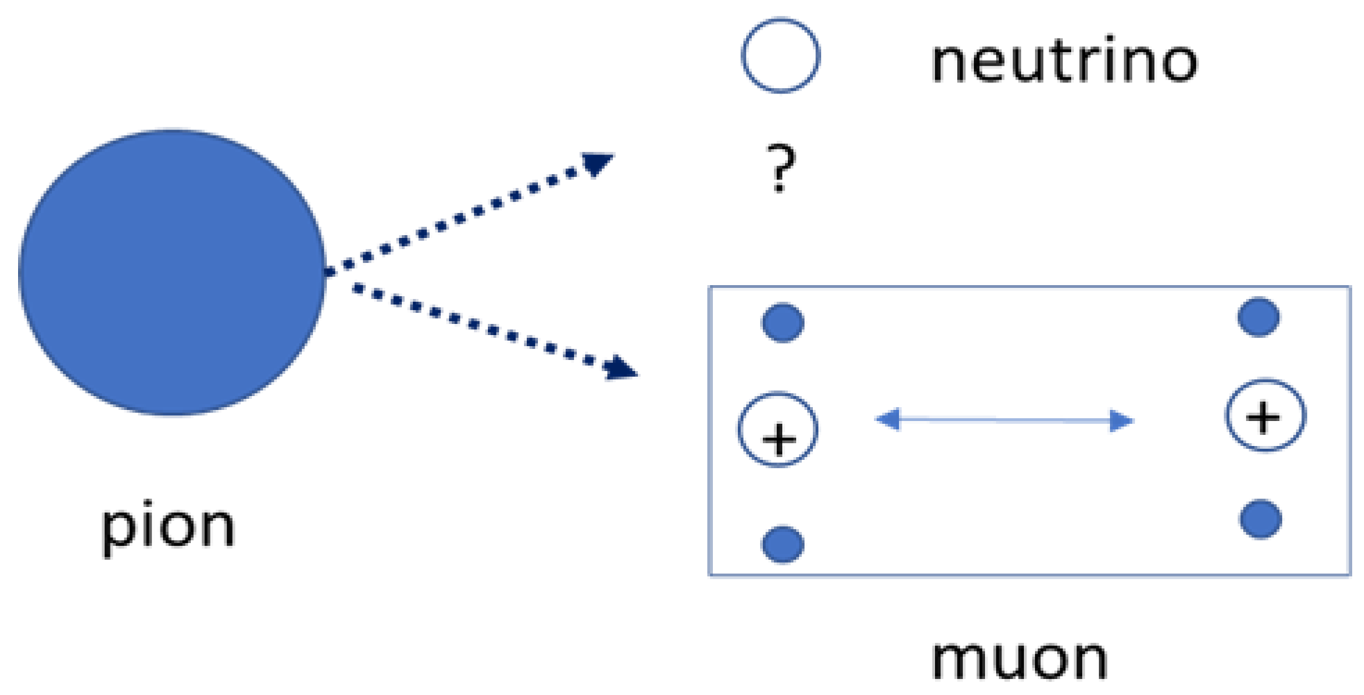
Figure 5.
The jump from the muon state to the tauon state is a jump from the first excitation level of the muon state to the ground state of the heavier tauon. It happens at a spacing d’ = 0.55, where the energy constants (not to be confused with the massive energies) match, under preservation of a slight amount of binding energy.
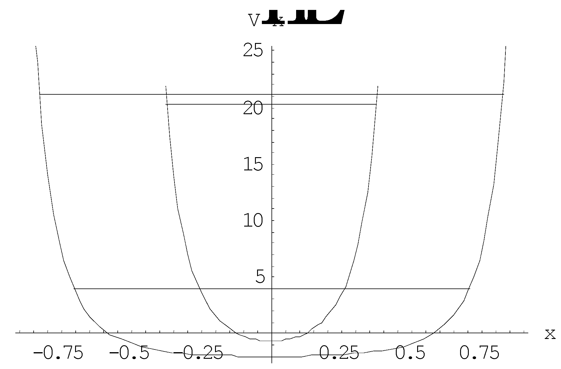
Figure 7.
The neutrino's pole spacing is determined by the equivalence of the vibrational energy of the neutrino's first excitation level, or the second excitation energy from the ideal ground state with its ground state vibrational energy at reduced pole spacing. Note that, unlike in the case of charged leptons, the binding energy (shown on a different scale as the lower curve) allows three modes of eigenstates instead of two.
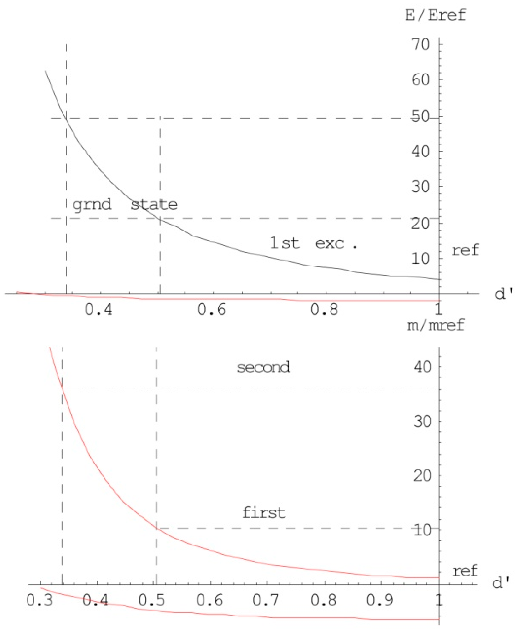
Figure 8.
Neutrino data.
Disclaimer/Publisher’s Note: The statements, opinions and data contained in all publications are solely those of the individual author(s) and contributor(s) and not of MDPI and/or the editor(s). MDPI and/or the editor(s) disclaim responsibility for any injury to people or property resulting from any ideas, methods, instructions or products referred to in the content. |
© 2025 by the authors. Licensee MDPI, Basel, Switzerland. This article is an open access article distributed under the terms and conditions of the Creative Commons Attribution (CC BY) license (http://creativecommons.org/licenses/by/4.0/).
Copyright: This open access article is published under a Creative Commons CC BY 4.0 license, which permit the free download, distribution, and reuse, provided that the author and preprint are cited in any reuse.


