Submitted:
29 March 2023
Posted:
29 March 2023
You are already at the latest version
Abstract
The phenomenon of dissipative self-organization is studied on the example of time-crystal networks. Particular attention was given to transient processes, attractor topologies, phase transitions, and asymptotic stability. New concepts were introduced, including topological phases, spinorial states, and bond flavors. Concepts such as ground states, chemical potentials, elastic forces, temperature, and statistical distributions were endowed with a new meaning associated with asymptotic stability. Phenomena usually attributed exclusively to quantum physics have been shown to occur in this essentially classical environment. They coexist with, and in some cases, such as charge quantization, are related to the phenomenon of time dilation. The approach was applied to model vacuum self-organization. We have shown that under the ac-tion of competing forces, such as gravity and antigravity, a cascade of phase transitions can transform an unorganized vacuum into phases in which interactions, fields and waves resemble electromagnetic, weak, and strong, and their elements can be used as building blocks for prototype particles. In addition, some interrelation field parameters and probabilities of particle transmutations were calculated, which are not predicted by the standard model. The results are consistent with the experiment. The presented material and methodology may be of interest for studying self-organization in different environments.
Keywords:
dynamical systems
; self-organization
; temporal periodicity
; attractor topology
; phase transitions
; synchronization patterns
; physical vacuum
; elementary particles
; unification of forces
1. Introduction
Most physical theories are based on the principle of energy conservation, which is applicable to strictly closed systems. Here, we will focus on the systems where energy is not conserved. We call them open. Most open systems do not hold their energy and dissipate it into the environment. However, some, under certain conditions, can stabilize, compensating for the loss of energy by extracting energy from the environment. This is possible if the environment is far from thermodynamic equilibrium and is controlled by nonlinear forces through feedback loops. We classify such open systems as self-organizing and focus mainly on their evolution and temporal properties.
The recurrent action of the feedback loop can lead to the establishment of periodic system dynamics. Temporal periodicity is the simplest form of self-organization. Nature as well as technology gives us numerous examples of self-oscillating systems: pulsars, von Karman vortices, color-changing chemical reactions, living cells, biological organs (hearts, lungs, intestines, brains), songbirds, choruses of cicadas, human societies, organ pipes, electronic signal generators, lasers, and so on.
Crystal implies periodicity, and time crystal signifies temporal periodicity. The name “time crystal” was coined by Winfrey [1] for a special case not directly related to our study. Almost from the very beginning, the time crystal concept caused controversy [2,3,4,5,6,7]. To avoid confusion, here, we will only consider systems that generate unaided periodic behavior. They are known by various names: self-sustaining oscillators, self-oscillators, autogenerators, orbitally stable limit cycles, vortices, rotators, and others. For brevity, we will call them all oscillators. They should not be confused with conserved oscillators or damped oscillators, which are of little interest to us here and which we address to resonators. We also exclude oscillating systems driven by any type of external periodic force, such as those described in [5,7,8,9].
As we shall see, temporal periodicity is not the only “crystal” property of time crystals. We will encounter different types of time-related symmetries, phase transitions, inhomogeneities, waves, defect transfers, etc. These properties will be discussed in Section 2, Section 3, Section 4, Section 5 and Section 6.
Strictly speaking, any system about which we receive information is open because its communications are nothing else as energy exchanges. In some cases, such a system can be conditionally considered closed. This is a case if, for example, such a system, after its birth, can reach a stable state and maintain its energy at a fixed level, and we are not interested in the details of its origin or “metabolism”. However, the true nature of the system is revealed after a brief disturbance brings it out of equilibrium. Then, if the system remains closed after the perturbation, it will remain in the state into which the perturbation brought it, and if the system is dissipative, then it will return (relax) to its original state. In the latter case, stable dynamic equilibrium is an asymptote or attractor, and the trend to return to this state is associated with asymptotic stability.
Let us take an electron as an example. Initially, after the discovery of the particle, it was believed that it has fixed internal characteristics, such as charge, mass, and angular momentum. The fixed values agree well with the assumption that the electron is a closed particle. However, it was later recognized that when an electron is perturbed, its charge and other characteristics can change. The charge is running, and only its equilibrium value is a constant. This value clearly has the properties of an asymptote or attractor: the electron returns to this value regardless of its previous history, details of origin, or level of excitation. The asymptotic stability of the electron charge indicates particle openness. In quantum electrodynamics, based essentially on conservative principles, the electron openness infiltrates the theory as a cloud of randomly popping up virtual particles surrounding the electron core. The cloud size and the virtual particle energy are arbitrary. The latter briefly violates the law of conservation of energy, and virtual particles quickly dissolve in the vacuum. However, it is the cloud that largely determines the magnitude of the asymptotic charge and other properties of the electron and imposes asymptotic stability on it.
Yes, we will consider the electron in this paper, but not as an independent object, but as a component of a multilevel and multifaceted self-organizing structure that arises in a nonlinear dynamic vacuum far from thermodynamic equilibrium. We will observe how various time-crystal networks arise in vacuum and endow it with the properties of fields and particles, in many respects similar to the properties of objects in the standard model. Section 7, Section 8, Section 9, Section 10, Section 11, Section 12 and Section 13 are devoted to this.
Numerical simulations were carried out using the formalism of iterated maps [11,12,13,14]. The evolution of iterated maps is very similar to the evolution of nature. Both are aimless and ignorant of possible outcomes. After running all possible histories, the “proper” one was selected based on the highest asymptotic stability. We will use this as natural selection.
Some ideas and results relevant to this study (but without mentioning time crystals) were published by the author in [15] and a few preprints.
2. Parameter as a measure of asymptotic stability
The typical oscillator evolutionary trajectory in the state space is a spiral that can start at any available point (state) and asymptotically approaches an exponential curve, which, in turn, converges to an asymptote – a closed curve called an attractor:
where is the absolute value of the distance between the spiral and its attractor in the state space and is the convergence time constant, which we will also refer to as the relaxation time.
Asymptotic stability is one of the main properties of dissipative systems, including self-oscillators. Regardless of their starting points, all spirals converging to the same attractor do so with the same time constant, and we use the latter as the attractor characteristic and as a measure of the asymptotic stability of the corresponding equilibrium states. Attractors with a minimal time constant will be called superattractors or the system ground states.
In this study, we will look for the most stable states and trajectories leading to them. In conservative systems, the most stable states are those with the lowest energy, and the “proper” evolutionary trajectories are those with the least (stationary) action. In open systems, energy is not conserved and is generally poorly defined due to the blurring of system boundaries. Therefore, instead of energy, we have turned to asymptotic stability and will use one of its characteristic parameters, which we call the stability parameter and define as
Our choice is not accidental. The parameter has some similarities with energy. For example, it is expressed in the same units (frequency) as energy in the system of units, where . The self-sustained oscillator is a self-bound system, and similar to energy in bound systems, is negative. Below, instead of the principle of least energy or action, the principle of least will be used. The similarities do not end there, and we will emphasize them as they appear in the text.
The generally recognized characteristic of asymptotic stability is the Lyapunov exponent . It is related to the stability parameter as the “action” accumulated over one cycle of oscillations:
Here, is the duration of one oscillation cycle. The second equality in (3) assumes that during one cycle, is a constant. In the ground states, is minimal, as it should be according to the principle of least action.
We also want the temperature to be expressed in the same units as the parameter . In a turbulent medium, oscillators jump from one evolutionary trajectory to another under the influence of random perturbations. The frequency of these jumps increases with temperature. We assume that the dependence is linear and define the temperature as the frequency of these jumps:
where is the average time during which the oscillator is continuously on the same trajectory.
We can roughly estimate the relative probability of the oscillator being in states with different values of the parameter . To do this, we note that there is a relationship between the uncertainty of the parameter and the lifetime of the state, similar to the time-energy uncertainty relation in quantum mechanics. This dependence arises in dissipative systems where trajectories starting at any point in the state space (which covers the entire possible range of values of ) converge over time to one state with a well-defined value of . The longer the evolution time on a given trajectory, the smaller the uncertainty of the parameter . On oscillator trajectories, the temperature-limited lifetime is . The state-space volume occupied by trajectories converging to the state initially covers the entire state space and decreases with time approximately exponentially and with the same time constant that its trajectories converge to the attractor. For simplicity, we will assume that the trajectories do not disappear, but their density in volumes increases in the course of evolution and that the probability of finding the oscillator in volume at time , when it is ready to switch to another trajectory, is proportional to the average trajectory density in this volume. Then,
and using equations (2) and (4), the probability
Considering the parallel between parameter and energy, expression (6) imitates the Boltzmann factor. Below, we will see how synchronization between oscillators turns this “classical” distribution into a “quantum” distribution.
3. Connected time crystals
From now on, the word “phase” will be used in two different senses: as a state of existence (such as a topological phase, vacuum phase, phase transition) and as a temporary phase, i.e., the fraction of a cycle in a periodic process (such as a phase difference, phase shift, phase entrainment). Usually, the meaning is clear from the context; otherwise, it will be provided.
Weakly coupled oscillators evolve asynchronously. They have different periods and disconnected phases. A phase shift imposed on one of them does not change the dynamics of the others. This gauge freedom is lost when the oscillators interact more strongly and become synchronized. Synchronization is a phase transition that can take various forms [16,17,18]. Below, we will provide two examples: phase entrainment and amplitude quenching.
Phase entrainment (also known as phase locking) is a ubiquitous phenomenon that can occur between oscillators of the same type, as well as between oscillators that produce different waveforms (regular or chaotic), have different designs, and even use different principles of operation. Phase locking transforms the coupled oscillators into a coherent network, where the phases of the oscillators are tied to each other, and the oscillator phase differences emerge as an order parameter. The network -values form a field on the network, which we call the -field.
Phase-locked oscillators also lose frequency independence. After synchronization, their continuous spectrum becomes discrete, often consisting of only one line. In what follows, for simplicity, we will assume that the latter occurs by default.
Oscillator networks can be viewed as graphs, where oscillators occupy nodes, and bonds are represented by the links (edges) between them. The graph links are “weighted” by the phase difference (in the process of link evolution) or (after relaxation) and can themselves be considered self-organized systems. We will model their dynamics using the Adler equation [19], which we have adapted [15] to the formalism of iterated maps:
Here, is the oscillator cycle duration after synchronization, and are the phase differences between the oscillators at times and , separated by one cycle (time interval ); is the difference between the oscillator frequencies before synchronization (natural frequencies), and is the engagement coefficient, which characterizes the coupling strength between the oscillators and varies from (uncoupled) to (fully engaged).
Examples of phase-difference evolution trajectories, calculated using the iterated map (7), are shown in Figure 1(a). They illustrate the quantum property of dissipative systems that we have mentioned in the previous section: regardless of the initial phase differences , which occupy a continuous interval, they asymptotically converge to one of the fixed values , which are determined by the parameters ∆ω and κ. The trajectories asymptotically become exponential with time (Figure 1(b). Accordingly, for link characterization, we use parameters similar to the oscillator parameters , , and , given by formulas (1)-(4), as well as the statistical distribution (5).
Examples of plots simulated using iterated map (7) are shown in Figure 2. All ground states (minima) correspond to oscillators operating in unison, .
The ground states are the most stable. Links tend to gather near those, while environmental disturbances move them out. In addition, they repeatedly return to the ground states. This trend can be formalized by introducing elastic (restoring) forces , which we define as
Elastic forces form the -field on the network. This field can be considered gauge if we pretend that the network has local gauge freedom and that the field arises as a network response to arbitrary changes in phase differences .
Under the action of the elastic force, the link changes the value of not instantly but with some relaxation delay, which plays the role of inertia. As a result, elastic forces cause wave-like oscillations in the medium. The amplitudes of these waves are the phase differences , which should not be confused with the wave’s own phase. This type of excitation is known as phase waves [20]. We call them -waves.
Near the ground states, the dependences can be approximated by quadratic parabolas (an example is shown by the green dotted line at the bottom of the curve in Figure 2):
where is the ground state value and is a parameter, we call the stiffness factor. For weak engagement, when , . For stronger engagements, increases faster than , and for full engagement, when , .
Accordingly, with a small deviation from the unison, the elastic forces are proportional to the phase difference :
and -waves are harmonic. Equation (10) plays the role of Hooke’s law for oscillator links. If the linear approximation (10) is violated, other types of waves can arise, including solitary waves [21].
The nonlinear behavior of the elastic forces is illustrated by the graphs in Figure 3 in normalized coordinates. With the departure from the ground state, Hooke’s growth slows down, then it is replaced by saturation and (at sufficiently large ) a falling branch (Figure 3). As increases, the positions of the maxima of the curves approach the ground state , and at , the ascending segment and saturation disappear, and only the descending branch remains. If we recall the parallel between the parameter and energy, then the softening of the force with increasing excitation, described by descending branches, resembles the behavior of color forces in chromodynamics, known as asymptotic freedom.
Dissipative systems are irreversible in time. Due to the lack of this symmetry, the time-crystal medium does not hold Lorentz invariance: irreversible time cannot be partially transformed into reversible space and vice versa. However, this does not prevent the medium from experiencing a universal time dilation, which is as profound as its counterpart is in relativistic gravity.
In time crystal networks, time dilation occurs in areas that move away from the ground state. It is directly related to slowing down relaxation. The time constant increases from the initial, ground state value and can progress to , which manifests a complete stop of the relaxation process. Time dilation concerns all processes in the affected part of the network. Looking ahead, we will model vacuum as a time-crystal network, where elementary particles and fundamental fields consist of connected network elements; thus, when excited, they experience time dilation. Any object that includes them as its parts will inherit this property. This applies to any type of clock/chronometer, even something as small and simple as an elementary particle itself.
It would be interesting to compare the time-crystal time dilation with the gravitational time dilation. To do this, let us compare the time dilation in a time-crystal link when it is excited from the ground state to the maximum excitation and the slowdown of a clock moving from infinity (ground state) to the black hole horizon . is the distance between the clock and the center of the black hole, and is the Schwarzschild radius. The normalized gravitational time dilation as a function of normalized excitation was extracted from the Schwarzschild metric and is given by the formula
It is shown in Figure 4 by the blue curve. The normalized time-crystal time dilation vs. the normalized link excitation simulated with use map (7) is shown in the same figure by the red curve.
In time-crystal networks, phase entrainment equalizes the oscillation periods of all synchronized oscillators, and the resulting period unified plays the role of a global invariant. The local relaxation time can be measured in -units and used to uniquely determine the local time metric. This is also applicable to vacuum if it is a time-crystalline medium. However, since temporal periodicity does not entail spatial periodicity, there is no object that could play the role of a standard of spatial distance. Instead, we can use spatially extended objects, such as -waves, and, borrowing a postulate from the theory of relativity, endow all -waves with the same propagation speed . Then, the product can be used as a standard of spatial distance. Its size will follow the local time changes, as it does in Minkowski spacetime. However, it should be remembered that the link between spatial and temporal metrics is not an emergent property but is introduced a priori. Fortunately, our analysis of the time-crystal media does not include spatial distances.
Synchronization occurs as a trade-off between coupled oscillators, each trying to make the other oscillators operate in the same mode as itself. Their struggle is accompanied by positive feedback: the more oscillators operate in a given mode, the greater they attract other oscillators to this mode. Let us see how this changes the probability distribution (see also [15]) given .
Suppose that the probability that an oscillator is in state increases linearly with the number of oscillators already in that state, and is the proportionality factor. Then, the synchronization-altered probability can be written as
where is the probability before synchronization. After separation of variables
Using expression (5) for the probability in equation (13), we obtain the final expression for the probability distribution:
where is a coefficient depending on . The distribution (14) has a form similar to that of the Bose‒Einstein distribution.
Amplitude quenching [16] is synchronization, in which the amplitude of the synchronized oscillators is reduced to zero. The affected oscillators group in the zero-amplitude state. In fact, they remove each other from the network.
To see how amplitude quenching will affect the statistical distribution, we can repeat the previous reasoning by making the following substitutions in equations (12)-(14): to distinguish between two synchronization scenarios, use index “” instead of index “” and instead of the proportionality factor use . Then, the probability, modified by the damping of oscillations, is equal to
which leads to the final distribution in a form similar to the Fermi-Dirac distribution:
where is a coefficient depending on .
It is noteworthy that, in contrast to quantum mechanics, quantum-like distributions (14) and (16) were obtained without the a priori assumption that the oscillators are indistinguishable from each other. Their alikeness is emergent.
4. Time-crystal phases with different attractor topologies
Under certain conditions, oscillators experience period doubling. This is a temporal phase transition accompanied by a symmetry break between the oscillator cycles. Theoretically, an oscillator can experience an infinite number of period doublings, a sequence that eventually drives it into chaos. After the first period doubling, the symmetry between even and odd cycles is broken. After the second period doubling, this happens between the 1st and 3rd cycles and between the 2nd and 4th cycles in each period of four cycles. The period doubling cascade follows certain patterns known as the Feigenbaum universality. However, in practice, chaotic dynamics appear after just a few period doublings.
The phases separated by period doubling differ in many properties, but perhaps most of all in the topology of their attractors. For brevity, we will call them topological phases. Some important qualitative differences between topological phases are illustrated in Figure 5. The attractor winding number is a phase hallmark. It is the number of attractor loops, which is also equal to the number of different cycles in one period. Due to the closeness of the attractor curve, is an integer.
We call oscillators with regular. Oscillators with have some spinor properties in the sense that in order for the oscillator to return to any of the previous states, it must complete two or more revolutions around its attractor. We call the corresponding topological phases and oscillators spinorial. Different loops/cycles represent different spinorial states of the oscillator. Spinorial states are dynamic and replace each other in a certain order. In Figure 5, we conventionally marked different spinorial states with different colors. In the spinorial phase , the sequence of colors is , and in the spinorial phase , the sequence of colors is . This color code will be used throughout the paper.
Spinorial states become especially important when the oscillators synchronize their dynamics (see below). Then, their synchronization patterns can become confusing. To prevent this from happening, we will use a special type of diagram [15], which we call spinorial clock diagrams (Figure 5, right column). Naturally, the spinorial clock diagrams are dynamic. They rotate synchronously with the spinorial states (Figure 6(a)). The direction of rotation is counterclockwise and irreversible in accordance with the irreversibility of the time arrow. The current state corresponds to the twelve o’clock mark.
A glitch in the spinorial color sequence caused by an external disturbance that shifts the cycle sequence by will be called a temporal. An example of a temporal shift by is shown in Figure 6(b), where the cycle is followed by a cycle instead of . We will use temporal dislocations to describe one of the possible mechanisms for changing the flavor of particles and to estimate their probabilities.
Phase transitions with period doubling significantly change the oscillator dynamics, their statistical distributions, chemical potentials, elastic forces, and other properties. For example, Figure 7 schematically shows the profiles of parameter in different topological phases. Here, is the control parameter, which we will acquaint with in Section 7, where specific simulation results will be given.
We will use spinorial oscillators as the building blocks of elementary particle prototypes.
5. Link flavors
Oscillators in spinorial phases can be synchronized in the same spinorial states (such as -, Figure 8(a), ) or different (such as -, Figure 8(a), ), and the dynamics of the - link are so significantly different from the dynamics of the - link that we consider them to be different dynamic systems. However, the same link that is currently - (Figure 9, ) will be - in the next cycle, then -, and so on. However, it will never turn -. To avoid confusion, it is helpful to use spinorial clock diagrams, as we did in Figure 8 and Figure 9. We will distinguish links as different if they do not have the same color combinations, regardless of which cycles the comparison is made in. We call them links of different flavors. Each flavor will be assigned its own flavor number , which is the phase shift between the coupled oscillators, expressed in number of cycles, , where the count starts from the monochrome links ().
If we take any spinorial oscillator, its spinorial states quickly replace each other, and each of them is not its specific characteristic. In contrast, the link flavor emerges in phase-entrained oscillators as a stationary parameter characterizing the spinorial pattern of their synchronization. Each of the oscillators represents a spin state frame for the other. This is reminiscent of a quantum mechanical spin, the direction of which only makes sense with respect to the frame of reference.
The significant differences between links of different flavors are illustrated by the following simulations. We have used a modified iterated map (7) with added spinorial subharmonic terms. We used iterated maps (17) and (18) for and links, respectively. The second and fourth subharmonic contributions are taken into account by their respective weighting coefficients and .
Links with the same parameters and and the same weighting coefficients and but having different flavor numbers have different attractor basins and converge to different fixed points (Figure 8(a). More importantly, their asymptotic stabilities and hence relaxation times (Figure 8(b)) and parameters and are also different. They also have different - and -profiles, ground states, and elastic forces (Figure 9).
In spinorial networks, -fields arise from the same premises as in networks consisting of regular oscillators. However, in spinorial networks, due to the variety of spinorial states and bond flavors, -fields have more degrees of freedom and additional symmetries. This complication is reminiscent of the complication that accompanies the transition from an electromagnetic field to a weak or strong field and can be formally described using additional state-space dimensions or using a fiber bundle construction.
6. Tunneling and entanglement based on phase correlation
In Section 2, using iterated map (7), we found that the most asymptotically stable links are those with the minimum phase difference between the oscillators. The conclusion was made without reference to the distances between the oscillators. Therefore, it is valid both for directly related oscillators and for oscillators that are far from each other. More stable links imply a higher degree of correlation between oscillators. In branched networks, due to interactions realized through parallel channels, the correlation between oscillators far from each other can be even higher than the correlation between nearest neighbors. Such counterintuitive behavior was observed in [22]. One of the networks from [22] is schematically shown in Figure 10(a). The network topology is a hypercube. Each edge represents a chaotic pulse generator. A network fragment consisting of three connected edges is shown in more detail in Figure 10(b). A typical pulse train from generators is shown in Figure 10(c). Coupling between autogenerators is regulated by resistors . The signals were measured in resistor nodes (black circles with numbers from 1 to 8). A typical set of correlation functions between the resistor node 1 and the other resistor nodes is shown in Figure 10(d). Between node 1 and the most distant node 8 (black curve), the correlation is much stronger than that between node 1 and any other resistor node (color curves). Similar “anomalies” were observed with other selected sets of resistors, as well as in branched networks with other circuit topologies.
A more stable long-range link can be established through the parallel channels provided by the less stable short-range links. This phenomenon in networks of time crystals may be responsible for behavior that mimics quantum tunneling and entanglement. Let us explain this by the example of the hopping mechanism of the transfer of a spinorial defect.
Here, a spinorial defect is an oscillator in the spinorial phase surrounded by a network of regular oscillators. We emphasize that the spinorial phase is an excitation and can move along the network, hopping from oscillator to oscillator, while all oscillators remain in their original places. We will not be interested in short hops between neighboring oscillators but in long hops between distant oscillators. Three stages of spinorial defect transfer are illustrated in Figure 11: before the transfer (Figure 11(a)), during the transfer (Figure 11(b)) and after the transfer (Figure 11(c)). The oscillators in the spinorial phase (before and after transfer) are shown by the red circles, all excited oscillators involved in transfer are shown by the white circles, and nonspinorial oscillators in equilibrium are shown by the black circles. The initial defect position is marked with the letter “I”, and the final defect position is marked with the letter “F”.
The role of the excited oscillators, shown by white circles, is to form a stable connection between the I- and F-oscillators through parallel channels. All of them are defect transmitters. During the transition, the defect is in the virtual state. It does not have a specific location. It is smeared over “white” oscillators, which are in an intermediate excitation state, neither spinorial nor regular.
Until the complete transition of the defect, its position is not determined. It can land on any of the excited oscillators. The noisy environment randomizes the result. However, since the most stable and rapidly relaxing links imply that their oscillators operate in unison (), the most likely location for the endpoint of a hopping defect is an oscillator with a temporal phase closest to the I-oscillator.
If the excitation of oscillators occurs much faster than their relaxation, then we can assume that they are excited simultaneously (in parallel). Then, the duration of the long jump of the defect may turn out to be shorter than the time required for the passage of the -wave sequentially from neighbor to neighbor. This will look like a violation of the relativistic principle of locality.
Quantum entanglement is realized when two spinorial defects tunnel from the same location I to two distant positions F1 and F2 (Figure 12). Then, to find the most likely locations of F1 and F2, we can use the same reasoning as in the previous case and find that each of the F-oscillators is strongly phase-correlated with the I-oscillator and thus phase-correlated with each other. It should be emphasized that the correlation between entangled spinorial defects occurs not because they carry some hidden parameters but as a result of the interactions and “negotiations” between all involved network oscillators.
7. Vacuum as the time-crystal medium
We briefly reviewed the main properties of time crystals and their networks. Starting with this section, we will explore the properties of a hypothetical medium that we call the time-crystal vacuum. This part is self-organized and much smaller than the rest of the vacuum, which is not organized. The latter represents a gigantic reservoir with which the time-crystalline vacuum exchanges energy. We assume that both parts are far from thermodynamic equilibrium, controlled by nonlinear forces, and possess all necessary for temporal self-organization.
We will model vacuum (see also [15]) based on the following assumptions. Vacuum is dust whose particles interact with each other. The interaction occurs under the action of two types of mutually antagonistic forces: self-attraction and self-repulsion. Self-attraction mimics the action of gravity. Self-repulsion mimics the combined action of self-diffusion and dark energy. These forces are responsible for the primary temporal crystallization of the vacuum and all subsequent phase transitions, which we will consider below.
Briefly, the initial temporal crystallization can occur as follows. Randomly formed dust clots due to self-attraction create local dust flows directed toward the centers of the clumps. The growth of the clots increases the dust attraction and increases the centripetal flows, which further increases the sizes of the clots. This positive feedback would lead to gravitational collapse if it were not for centrifugal flows due to self-repulsion, which also increase with the growth of clots. Self-reinforcing radial flows in mutually opposite directions are unstable to flow fluctuations in transverse directions. In the end, they separate in space and form vortices similar to Bénard cells [23] both in form and in the ability to experience period-doubling phase transitions [24].
Emergent in a turbulent medium, the vortex dynamics are essentially stochastic. We will define as the probability that the radial flows in a vortex are predominantly centripetal and as the probability that they are predominantly centrifugal and assume that for small increments of time , the probability changes as
where is the medium amplification coefficient. Vortices emerge and can be maintained by the medium if .
Below, instead of and , we use parameters and , which we call the convergence and feedback control parameters, respectively, and define them as
To describe the development of vacuum vortices, we will use iterated maps [14], which are ideal for simulating aimless evolution. As a natural selection, we will compare the rates of convergence to attractors of all possible evolutionary trajectories and choose the most rapidly convergent ones, which are also the most asymptotically stable. Using the variables and , we rewrite equation (19) in the form
where sampling occurs at times and separated by the time intervals equal to the effective vortex rotation period , and the iteration function is
Function (23) is even in the variable . We use this property to introduce antimatter. We define antimatter vortices as matter vortices with reversed radial flows (). This is equivalent to a swapping of self-attraction and self-repulsion forces. Time remains irreversible.
Accordingly, the antimatter vortex evolution iterated map is negative of map (22):
Below, we will use their combination
where “” and ““ stand for matter and antimatter, respectively. On spinorial clock diagrams, we distinguish matter from antimatter by the colored rims: black and red, respectively, as shown in Figure 13.
8. Topological phases of self-organized vacuum
The results in this section were obtained using map (25) for various values of feedback control parameter . The minimum number of iterations for each value of was chosen so that at the last iteration, the change in the variable did not exceed . The values of at the last iterations were taken as the values of fixed points. It was assumed that these points belong to the corresponding spinorial states. Accordingly, the number of fixed points for each value of was equal to the attractor winding number . The relaxation time was determined near fixed points using equation (1). The time intervals between iterations were considered equal to . Parameters and were determined using equations (2) and (3).
The dependences of the fixed points and for matter vortices and antimatter vortices, respectively, are shown in Figure 14 by solid and dashed lines. Their graphs are mirror-symmetric with respect to the line . The diagram is called a bifurcation diagram. Bifurcations highlight phase transitions. For a self-organized vacuum, the diagram plays the role of a topological phase diagram. Our simulations cover three topological phases, which we call , , and . The names came from comparing them with electromagnetic, weak, and strong fields. We will also use quantum number to mark the respective topological phases as well as the ground states , attractor winding numbers , and bifurcations located to the right of the ground state with the same index. is a bifurcation corresponding to the initial temporal crystallization and a phase transition between unorganized and self-organized vacuum.
In Figure 14, the parameter scales are different in different topological phases to better illustrate the details of the plots. The colors of the branches correspond to the colors of the spinorial states in correspondence with the previously selected color code (Figure 5).
The initial temporal crystallization occurs at . Period-doubling phase transitions (bifurcations) occur at , , and . The intervals occupied by topological phases , , and are related to each other as
where is the Feigenbaum constant.
Dependence in three topological phases is shown in Figure 15 (see also [15]). Each topological phase has the form of a potential well with logarithmic-shaped walls:
where the discrete parameter plays the role of the chemical potential in the corresponding topological phase, which we define as
In equations (27) and (28), we neglected a slight asymmetry between the left and right halves of the wells in the topological phases and .
The ground states are located at , , and .
The distribution of vortices over was calculated using equation (6) in a normalized form:
where is the partition function. Using equations (27) and (28), the probability distributions can be explicitly expressed in each topological phase as
where is the partition function in the topological phase .
An example of the vortex distribution in parameter at a temperature is shown in Figure 16. This temperature is so high that the vortices only have time to complete five cycles before thermal noise knocks them off their trajectories. Even at such a high temperature, the vast majority of vortices are concentrated in the ground states and their vicinity. At lower temperatures, the linewidth sharply narrows, and the spectrum of the parameter becomes discrete. The same happens to the medium amplification coefficient . Other variables linked to are also quantized.
This also applies to the convergence . Recalling the operator form of the Gaussian law, one can notice a similarity between the negative convergence and the divergence operator. Using this analogy, we associate numbers with quantized vortex charges in the corresponding topological phases and spinorial states.
Taking into account twice-degenerated matter and antimatter “black” charges , the total number of vortex charges in each vacuum phase is . We compared them with the charges of the standard model bosons (Table 1). With one exception on each side, there is a one-to-one correspondence. The exceptions are in phase and the charge of the Higgs boson. Both are zero, and it is tempting to put them on the same line in Table 1 to achieve a perfect correspondence.
9. Relative strength of elastic forces in different topological phases
In Section 3, using equation (8), we introduced elastic forces for the oscillator links to formalize their tendency to return to the ground states. This applies to many dissipative self-organizing systems, including oscillators themselves and vacuum vortices. Thus, we define the elastic forces for vacuum vortices as
The elastic forces depend on the level of excitation (parameter ). For the same value of , they are different in different topological phases, and we will compare them under such conditions. Fortunately, we do not have to choose at what level of we want to compare forces. Due to the logarithmic shape of -well walls (see Figure 15 and equation (27)), and using equation (28), one can find that for any two topological phases and , the ratio between their elastic forces does not depend on the choice of and, taking into account relation (26), for any fixed , the forces are related to each other as
After substituting the numerical values in (32), we find that the elastic forces in , and are related to each other as:
It would be interesting to make similar comparisons between electromagnetic, weak, and strong interactions. The standard model does not predict field strength. Instead, it uses the empirical values of the coupling constants , , and . We compared their values at the energy corresponding to the vector boson masses, and , recommended (they are not directly measured) by the Particle Data Group [27]:
The numbers in proportions (33) and (34) were rounded to two significant figures. Given that the standard model does not give any estimates, we can say that (33) and (34) are in good agreement.
10. Vacuum network
When the density of vortices reaches a level sufficient for their partial overlap, they exchange dust particles, which leads to their mutual influence and, ultimately, to synchronization of the vortex dynamics. The network acquires temporal coherence. A new order parameter arises in it: a phase difference between the vortices. -fields are formed in the network, and their excitations have the character of -waves. The complexity of -fields in different topological phases is different in accordance with their spinorial structure. We assume that most of the vortices are in the topological phase, and small groups of directly connected spinorial vortices in the and phases are impurities that we associate with elementary particles. Below, we will consider them in more detail.
The synchronized vacuum network has its own global and local time scales. The global time scale is based on a time interval , equal to the period of one of the network vortices and chosen as a reference. The local time scale is based on the local value of the link relaxation time . A comparison between the values of at different locations can be performed by comparing both with the global time etalon , an invariant for the entire network. Their values relate to each other as reciprocal Lyapunov exponents .
The network ground states are located at the minima of . They arise in each topological phase, where the temporal phase difference between the vortices is zero. These are zero-points for -fields. These are also zero-points of time dilation. There are no such differences between them, as there are between zero-points in quantum theory and relativistic gravity. Their energy is not equal to zero but represents a huge energy of an unorganized vacuum and is more reminiscent of the energy of the zero-field in quantum physics.
Temporal crystallization does not imply spatial periodicity. In terms of spatial order, the vacuum time-crystal network is more similar to a polymer.
11. Spinons
In a spinorial vortex, the directions of radial flows change rapidly. When immersed in the network, a spinorial vortex with rapidly changing radial flows creates a strong dynamic network perturbation, behind which the network barely has time to adapt its dynamics. However, if a second spinorial vortex is added to the first vortex in the same topological phase but with a spinorial state different from the first vortex, then the network perturbation will be significantly smoothed due to internal exchanges of flows between vortex-synchronized polychrome. Even greater smoothing can be achieved if the matter/antimatter nature of the second vortex is opposite to the first vortex. To prevent mutual annihilation of such a matter-antimatter pair, the vortices must still be in different spinorial states (synchronized polychrome). The requirement for polychrome synchronization (when the vortices are in different spinorial states) is akin to the Pauli exclusion principle. Below, we will consider only polychrome pairs. We will use them as the building blocks of prototype particles and call them spinons.
A pair of vortices extended along one of the spatial directions can form a more compact torus shape (Figure 17(a)), which is also more stable. In any section of such tori, the directions of circular flows in paired vortices are opposite to each other. They should not be confused with spinorial clock diagrams, which always rotate counterclockwise.
Below, we will use six types of spinons (Figure 17) (see also [15]). We will discriminate them by the flavors of their bonds (links) and the matter/antimatter nature of their vortices. Three types of spinons belong to topological phase (Figure 17(b)), and the other three belong to topological phase (Figure 17(c)). The spinon flavor names are shown above their spinorial clock diagrams.
The three -spinon flavors (Figure 17(a)): (both matter vortices), (both antimatter vortices), and (one matter vortex and one antimatter vortex). The first two, , carry charges. In each spinon, the polychrome synchronization gives the impression that the charge oscillates between the coupled vortices. In fact, there is no movement of charge. Accordingly, there is no relativistic restriction on the oscillation rate. However, the surrounding network responds to these apparent shuttle fluctuations of charge by forming circular electric currents around the spinon. The currents spontaneously break the symmetry. The direction of their rotation is determined by the details of their occurrence. Based on Table 1, we associate spinons with electric charges . Among all spinons, only these two are carriers of electric charges. The spinon is electrically neutral (after time averaging).
-spinons are also electrically neutral. They are pairs of one matter vortex and one antimatter vortex (Figure 17(b)). After time averaging, they are also colorblind. We named their flavors after the flavors of quarks, but with some caveats. We call the flavors “ or ”, “ or ”, and “ or ” and use the notation , , and , where stands for “or”. This means that unperturbed -spinons and -spinons are the same spinons (as well as and c spinons and and spinons). However, if the -spinon is coupled to the -spinon, the degeneracy between and (or alternatively between and or and ) is lifted. This is due to the mutual penetration of dust flows between the coupled -spinon and -spinon. As a result, both spinons become hybridized. The -spinon acquires the topology of the -spinon (four spinorial states), and the -spinon acquires a part of the charge of the -spinon. The fractional charges resulting from this hybridization make hybridized spinons more like quarks.
Depending on the -spinon flavor, or , becomes or . The same happens with and . This is summarized in Table 2.
This can also be formalized by equation (35), where the sign denotes direct product, and the “” and ““ signs refer to matter and antimatter (not charge), respectively.
An example of a flavor change from positive to neutral is shown in Figure 18.
In the next section, we use spinons to synthesize prototype particles. The lepton prototypes will consist exclusively of pure -spinons, while the hadron prototypes will consist of mixtures of hybridized -spinons and -spinons.
12. Time-crystal particle prototypes
In this section, we will show several examples of particles built from spinons (see also [15]. To visually show the differences between the particles, especially their different flavors, we use spinorial clock diagrams. In the examples given, the variety of particles is due only to their composition and synchronization patterns (flavors). We have not addressed other possibilities to diversify the family of particles, for example, using differences in stereometry or in the mutual arrangement of vortices.
The prototype leptons are shown in Figure 19. Each particle of the first generation (Figure 19(a)) is represented by one of the mentioned -spinons. The second generation (Figure 19(b)) and the third generation (Figure 19(c)) are assembled by adding one and two -spinons, respectively, to each particle of the first generation. This does not affect the particle charge values but adds to their energy (mass). The internal particle fields are rapidly oscillating -fields of the -type and play the role of weak nuclear fields. They are inherently localized inside the particles.
The eight prototype mesons shown in Figure 20 mimic the Gel-Mann “eightfold way” meson set. They consist of one of three hybridized -spinons and one of hybridized -spinons, or. They can be considered second-generation leptons where one electrically neutral -spinon is replaced with one of the -spinons. The internal particle fields, taking into account the hybridization of -spinons, are -fields of the -type and play the role of strong nuclear fields. As in the previous case, they are localized inside the particles. The electric charges of the hybridized spinons are redistributed among all spinons and become fractional, while the total particle charges remain integer.
The eight prototype baryons shown in Figure 21 mimic the Gel-Mann “eightfold way” baryon set. They consist of one of three hybridized -spinons and two of or hybridized -spinons. They can be considered third-generation leptons, where in each particle, two electrically neutral -spinons are replaced with two -spinons. Remarks on internal fields and charges are the same as in the previous case.
Figure 21 shows only particles of matter. They can be converted into antiparticles by replacing spinons with spinons.
The above examples demonstrate that the prototype particles have different symmetry, complexity and taxonomy compared to those of the real particles described in the standard model. Only four different types of vortices were used as particle/field compositional elements: two matter vortices with and and two antimatter vortices. Two more, with , are necessary to represent the electromagnetic field. For comparison in the standard model, the number of elements is a total of 61: 13 field bosons, 12 leptons and 36 quarks.
13. S-flavor rotations
In the final section, we will consider the flavor rotation model [15] of nonhybridized -spinons. In addition to the three polychrome flavors , and , we will also need unstable monochrome coupling, which we have designated flavor and which will play the role of a brief intermediate (virtual) state in flavor rotation dynamics.
The reason for the spinon flavor change is a temporal dislocation, which creates an unequal phase shift in coupled vortices. Without loss of generality, we assume that the perturbation affects only one of the two vortices, and for the second vortex, . This can happen as follows. The affected vortex is briefly moved from the original color-rich topological phase to the colorblind topological phase , and after time , it returns to the phase in the same spinorial state that it left, while the second vortex stays in the phase and keeps its usual pace. Being in phase is unstable, and the event probability exponentially vanishes with time :
where is the difference between “chemical potentials” in the two topologic phases, which plays the role of activation energy.
We assume that before and after temporal dislocation, the vortex bond is in one of the ground states (the well bottoms in Figure 9). Then, is equal to an integer number of spinorial states:
where is the cycle duration and is the number of spinorial states skipped by the affected vortex. We do not consider temporal dislocations with a duration of more than 3 spinorial states since they lead to the same flavor changes as short dislocations, but their probability is immeasurably lower.
From equations (28), (36), and (37), and taking into account relation (26),
and the event probability decreases with the number of skipped cycles by the affected vortex as
The direction of flavor rotation depends on the matter/antimatter nature of the affected vortex, as shown in the diagrams in Figure 22. Here, the initial flavors are marked with bold dots on arrows. The probabilities for all possible events, including the unstable flavor (shown in red), are tabulated in a matrix (Table 3). The odd rows start with flavor numbers and and reflect the events shown in Figure 22(a), and even lines begin with flavor numbers and and reflect the events shown in Figure 22(b). Because the effects caused by hybridization are ignored, the matrix is symmetric, and the rows and columns can be swapped.
After removing the red row and red column of unstable initial and final states, the matrix is reduced to a size of (the leftover matrix elements are shown in Table 3 in black).
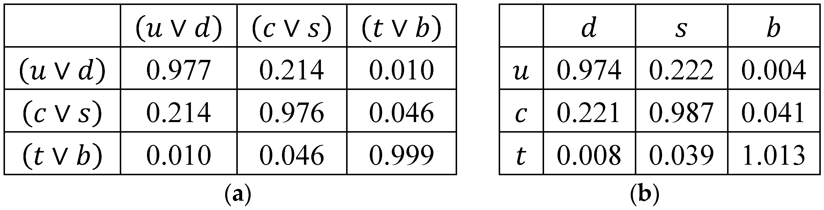
Now, we will compare it with the CKM matrix (Cabibbo-Kobayashi-Maskawa), which tabulates the quark mixing amplitudes obtained from experimental data. To make the comparison sensible, we need to bring the Table 3 matrix elements to the same form as the CKM matrix. To do this, we normalize the probabilities so that they satisfy the unitarity condition () in each row and each column, replace the normalized probabilities with their amplitudes (), and convert them into numbers.
The flavor rotation matrix after these manipulations is displayed in Table 4(a) next to the CKM matrix shown in Table 4(b).
All numbers in both matrices have been rounded to three significant digits, which is sufficient for their comparison. The matrix elements in the two matrices are not exactly the same, but the correspondence between their values and positions is obvious. It would also be interesting to compare both matrices with the predictions of the standard model. Unfortunately, as in the case of coupling constants, the standard model does not make such predictions.
14. Conclusions
We have considered the temporal aspects of self-organization in dissipative media far from thermodynamic equilibrium, consisting of asymptotically stable self-oscillatory systems (time crystals).
As open systems, time crystals cannot exist without their “metabolism” – persistent interactions with their environment. The process of their self-organization was modeled as evolutionary with numerical simulations performed with the use of iterated maps ideally suited for this goal. “Natural” selection was carried out by comparing all possible evolutionary trajectories and identifying systems with maximum convergence rates. The analysis was performed in terms of the specially introduced parameter , a surrogate for energy. The concepts of the ground states, chemical potentials, elastic forces, temperature, and some other physical characteristics as well as statistical distributions were given a new meaning in terms of this parameter.
A few new concepts have been introduced. Among them are topological phases, spinorial states, spinorial oscillators, spinorial defects, bond flavors, vortex charges, temporal dislocations, and spinons.
To avoid confusion, complicated synchronization patterns (bond flavors) of spinorial vortices were illustrated and analyzed using specially designed colored spinorial clock diagrams, which rotate synchronously with their spinorial states.
We have demonstrated that despite being essentially classical, the synchronized time-crystal medium produces a gamut of emergent properties usually a priori attributed to quantum objects. It is characterized by quantum numbers, discrete parameters, spinorial states, quantum-like statistical distributions, defect transfer hopping mechanisms imitating tunneling and entanglement, quantum-like uncertainty relations and other factors. The medium is time coherent. It can be described in terms of phase-different fields mimicking their structures of electromagnetic, weak, and strong nuclear fields.
On the other hand, being essentially time irreversible and nonrelativistic, the time crystal medium does possess the phenomenon of time dilation, and the latter is as profound here as it is in relativistic gravity. It is not only compatible with quantum behavior but in some cases is the reason for it.
In most cases, the time-crystal phenomenology we used is applicable to the medium where self-oscillators are substituted with rotators such as vortices. We use this fact to model the organized part of the vacuum as a time-crystal medium reserving for the rest of the vacuum the function of a huge energy reservoir that supplies free energy to the organized part. Vacuum self-organization occurs under the action of forces akin to gravity and antigravity (combined action of self-diffusion and dark energy). The competition of these mutually antagonistic forces leads to the formation (through different time-related phase transitions) of the abovementioned phase-difference fields with different structures. Most of the vacuum network represents a field that mimics electromagnetic fields. It consists of regular vortexes with an attractor winding number equal to . The fields formed by spinorial vortices with winding numbers and are interspersed into this medium as synchronized vortex pairs, which we call spinons. They are not only carriers of the corresponding fields but are also used to compose small aggregates of topological impurities with particle properties.
All vacuum fields have the same roots and can be transformed into each other (through period-doubling phase transitions). This unification allows one to model their relative strength, and the estimates are consistent with the experimental data. The model also allows for modeling spinon flavor changes. Their probabilities were found to be consistent with the CKM matrix tabulating empirically obtained probability amplitudes for quark flavor changes. None of them was made in the standard model.
The time-crystal network ground states mark zero-point vacuum fields as well as zero-point time dilation. This eliminates the huge discrepancy between zero-point energy in quantum physics and in relativistic gravity, known as the cosmological constant problem.
The presented model extrapolates the evolutionary approach to inanimate nature. We have considered only most elementary objects of the universe and only the temporal aspects of their self-organization. We hope that the methodology, analysis and results obtained can be used to study the phenomenon of self-organization at other levels and in other environments and domains.
Funding
This research received no external funding.
Acknowledgments
I am grateful to Lev Sadovnik and Vladimir Litvinov, who independently drew my attention to time crystals based on their acquaintance with my previous research.
Conflicts of Interest
The author declares no conflict of interest.
References
- Wilczek, F. Quantum time crystals. Phys. Rev. Lett. 2012, 109, 160401. [Google Scholar] [CrossRef]
- Shapere, A.; Wilczek, F. Classical time crystals. Phys. Rev. Lett. 2012, 109, 160402. [Google Scholar] [CrossRef]
- Bruno, P. Comment on” Quantum Time Crystals”: a new paradigm or just another proposal of perpetuum mobile? Phys. Rev. Lett. 2013, 110, 118901. [Google Scholar] [CrossRef]
- Bruno, P. Comment on “space-time crystals of trapped ions. ” Phys. Rev. Lett. 2013, 111, 029301. [Google Scholar] [CrossRef]
- Watanabe, H.; Oshikawa, M. Absence of quantum time crystals. Phys. Rev. Lett. 2015, 114, 251603. [Google Scholar] [CrossRef]
- Sacha, K.; Zakrzewski, J. Time crystals: a review. Rep. Prog. Phys. 2018, 81, 016401. [Google Scholar] [CrossRef] [PubMed]
- Khemani, V.; Lazarides, A.; Moessner, R.; Sondhi, S.L. Phase structure of driven quantum systems. Phys. Rev. Lett. 2016, 116, 250401. [Google Scholar] [CrossRef] [PubMed]
- Else, D.V.; Bauer, B.; Nayak, C. Cloquet time crystals. Phys. Rev Lett. 2016, 117, 090402. [Google Scholar] [CrossRef] [PubMed]
- Yao, N.Y.; Nayak, C. Time crystals in periodically driven systems. Physics Today, 2018, 71, 40–47. [Google Scholar] [CrossRef]
- Winfree, A. T. The Geometry of Biological Time. Springer, New York, 1980; p. 52.
- Peitgen, H.O.; Jürgens, H.; Saupe, D. Chaos and Fractals: New Frontiers of Science. Springer, New York, 1992.
- Strogatz, S.H. Nonlinear Dynamics and Chaos with Student Solutions Manual: With Applications to Physics, Biology, Chemistry, and Engineering. Perseus Books Publishing, New York, 1994.
- Hilborn, R.C. Chaos and Nonlinear Dynamics: an Introduction for Scientists and Engineers. 2nd ed. Oxford U. Press, Oxford, 2000.
- Collet, P.; Eckmann, J.P. Iterated Maps on the Interval as Dynamical Systems. Birkhäuser, Boston, 2009.
- Manasson, V.A. An emergence of a quantum world in a self-organized vacuum: a possible scenario. J. Mod. Phys. 2017, 8, 1330–1381. [Google Scholar] [CrossRef]
- Pikovsky, A.; Rosenblum, M.; Kurths, J. Synchronization: A Universal Concept in Nonlinear Sciences. Cambridge U. Press, New York, 2001.
- Strogatz, S.H. From Kuramoto to Crawford: Exploring the Onset of Synchronization in Populations of Coupled Oscillators. Physica D: Nonlinear Phenomena, 2000, 143, 1–20. [Google Scholar] [CrossRef]
- Balanov, A.; Janson, N.; Postnov, D.; Sosnovtseva, O. Synchronization: From Simple to Complex. Springer, Berlin, 2009.
- Adler, R. A study of locking phenomena in oscillators. Proc. IRE, 1946, 34, 351–357. [Google Scholar] [CrossRef]
- Yamauchi, M.; Nishio, Y.; Ushida, A. Phase waves in a ladder of oscillators. IEICE Trans. Fundamentals, 2003, E86-A, 891-899.
- Rosenau, P.; Pikovsky, A. Solitary phase waves in a chain of a autonomous oscillators. Chaos 2020, 30, 053119. [Google Scholar] [CrossRef] [PubMed]
- Manasson, J.; Manasson, V.A. Strange correlations between remote nodes in networks comprising chaotic links. 2015, arXiv:1511.02772 [nlin.CD].
- Bénard, H. Les tourbillons cellulaires dans une nappe liquide. Revue Générale des Sciences Pures et Appliquées, 1900, 11, 1261–1271. [Google Scholar]
- Libchaber, A.; Laroche, C.; Fauve, S. Period doubling cascade in mercury, a quantitative measurement. Journal de Physique Lettres, 1982, 43, 211–216. [Google Scholar] [CrossRef]
- Feigenbaum, M. J. Universal behavior in nonlinear systems. Physica D: Nonlinear Phenomena, 1983, 7, 16–39. [Google Scholar] [CrossRef]
- Cvitanović, P. (ed): Universality in Chaos. 1989, Routledge, New York.
- Zyla, P.A. et al. (Particle Data Group), Prog. Theor. Exp. Phys. 2020, 083C01, Available online: URL https://pdg.lbl.gov/; (accessed on 03/27/2023).
- CKM Quark-Mixing Matrix. Available online: URL https://pdg.lbl.gov/2020/reviews/rpp2020-rev-ckm-matrix.pdf; (accessed on 03/27/2023).
Figure 1.
Phase-difference evolution trajectories: (a) phase differences after the -th cycle; (b) the differences between current phases and their fixed points .
Figure 1.
Phase-difference evolution trajectories: (a) phase differences after the -th cycle; (b) the differences between current phases and their fixed points .
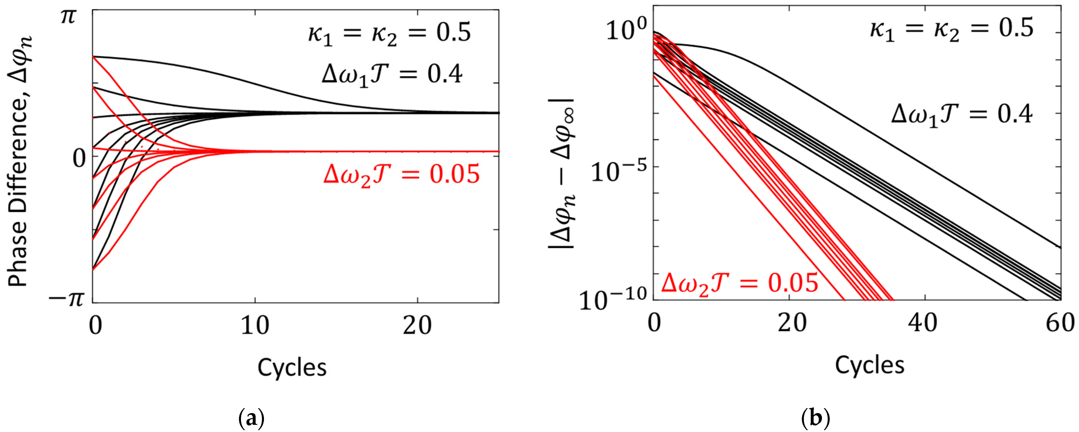
Figure 2.
for links with different values (solid lines). An approximation by quadratic parabola (dashed line).
Figure 2.
for links with different values (solid lines). An approximation by quadratic parabola (dashed line).
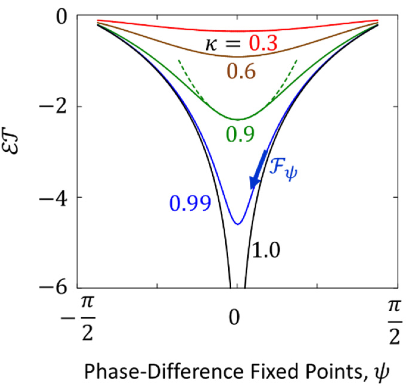
Figure 3.
Normalized elastic force vs. normalized parameter .
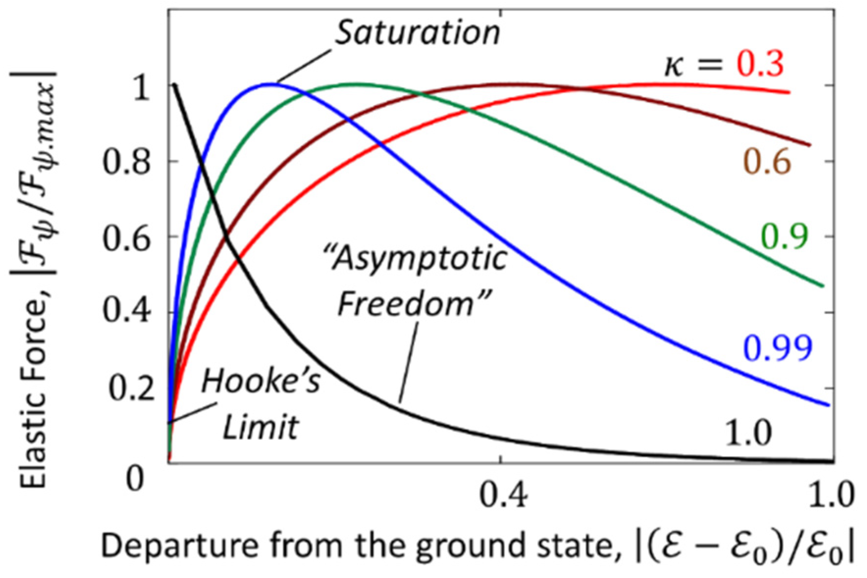
Figure 4.
Comparison between gravitational time dilation (blue) and time-crystal time dilation (red).
Figure 4.
Comparison between gravitational time dilation (blue) and time-crystal time dilation (red).
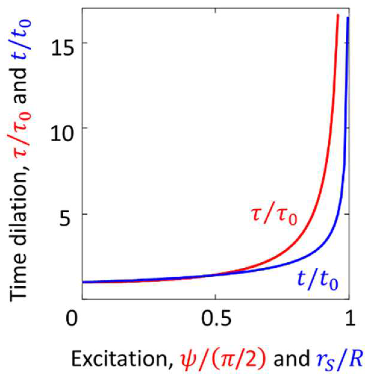
Figure 5.
Topological phases shown by different types of diagrams. Spinorial states are shown in different colors.
Figure 5.
Topological phases shown by different types of diagrams. Spinorial states are shown in different colors.
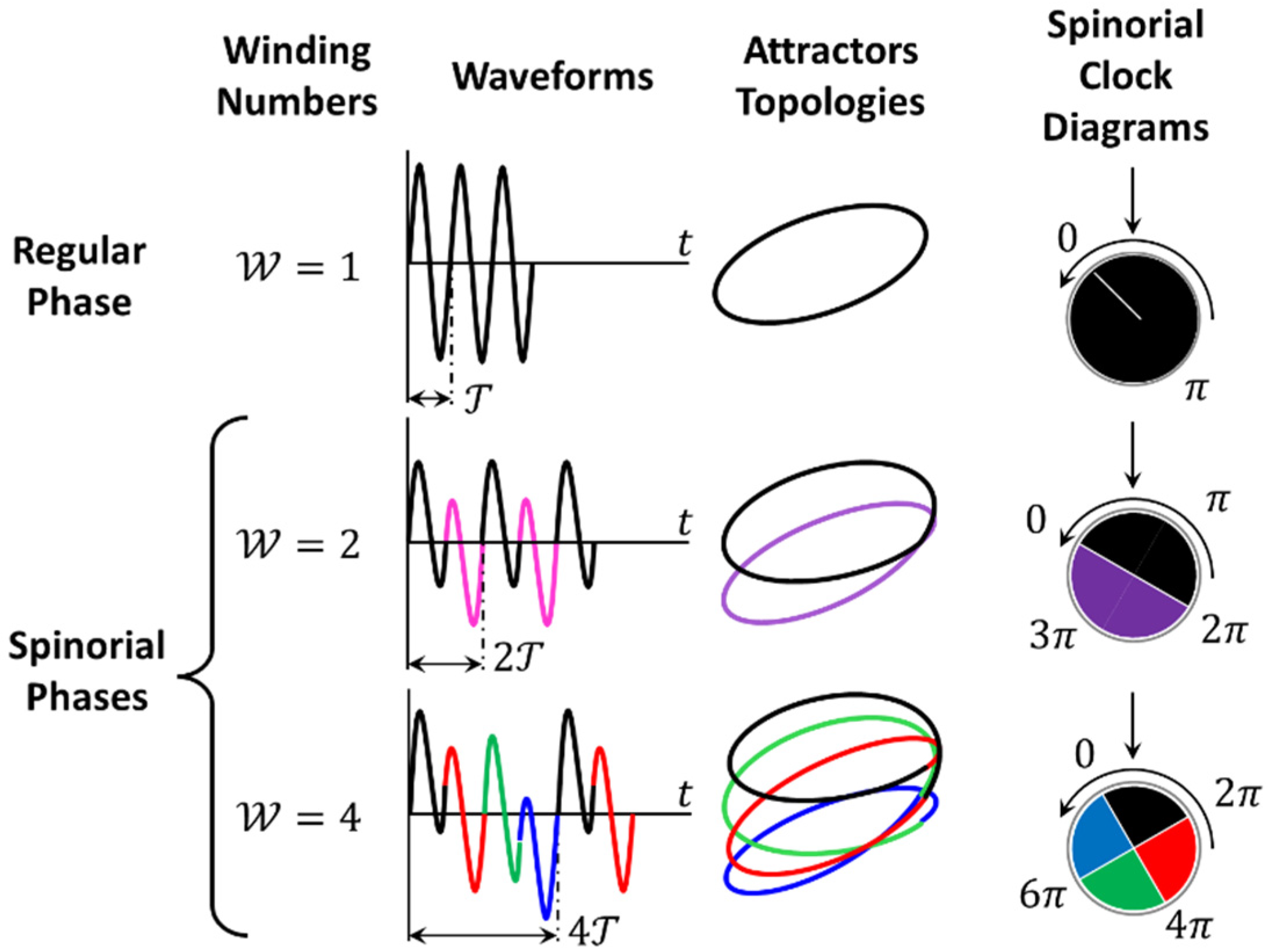
Figure 6.
(a) Example of spinorial clock diagram dynamics, is duration of one spinorial state; (b) A glitch in spinorial sequence equal to .
Figure 6.
(a) Example of spinorial clock diagram dynamics, is duration of one spinorial state; (b) A glitch in spinorial sequence equal to .
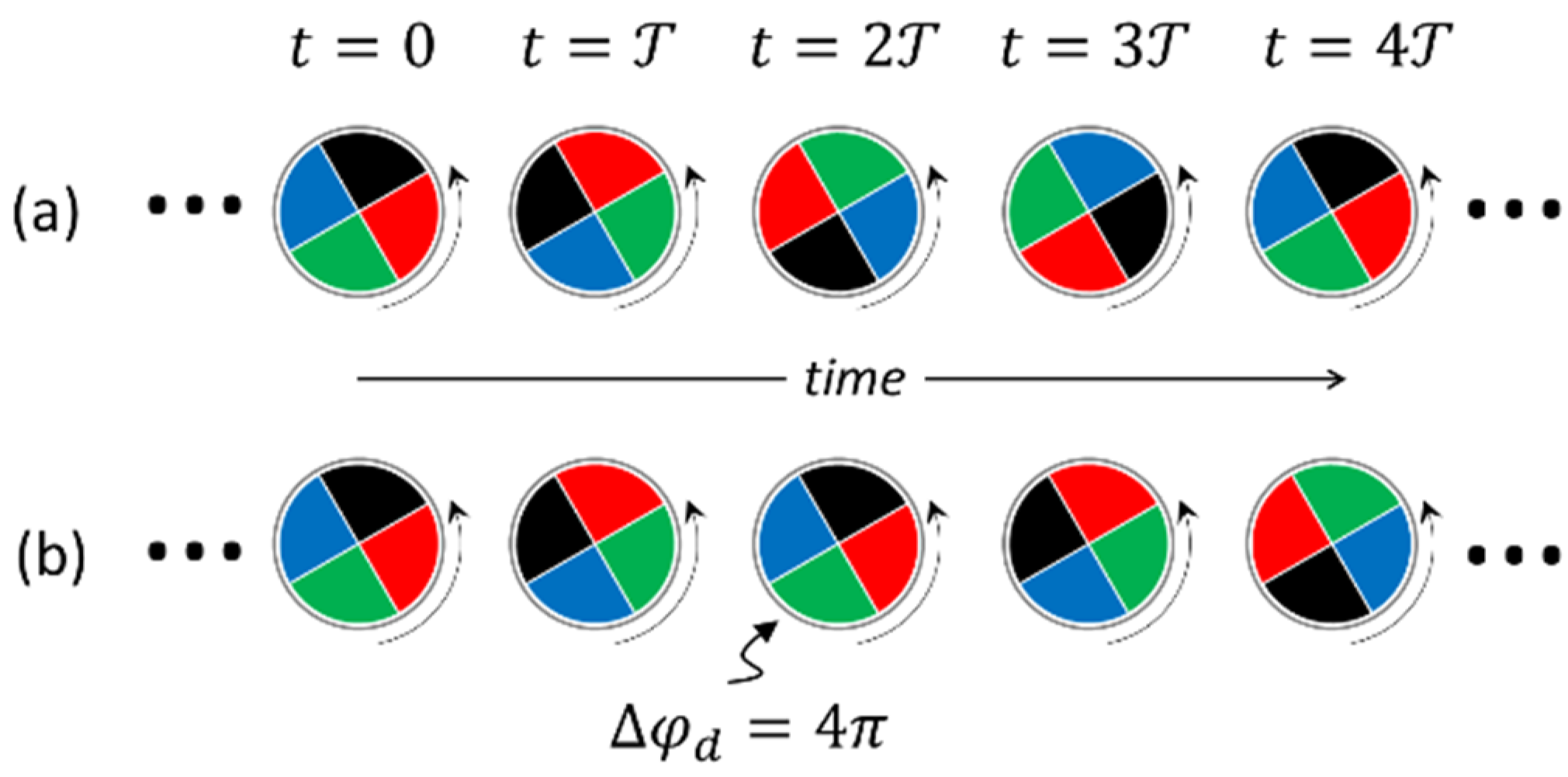
Figure 7.
-profiles in different topological phases.
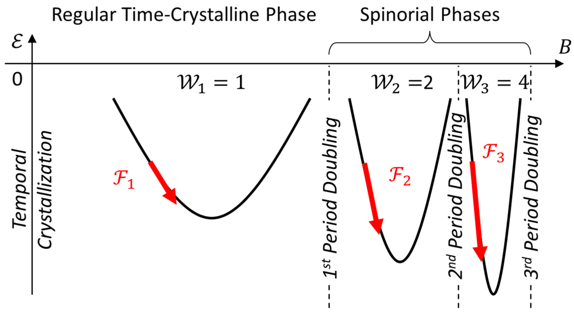
Figure 8.
bonds: (a) evolution trajectories; (b) convergence diagram. .
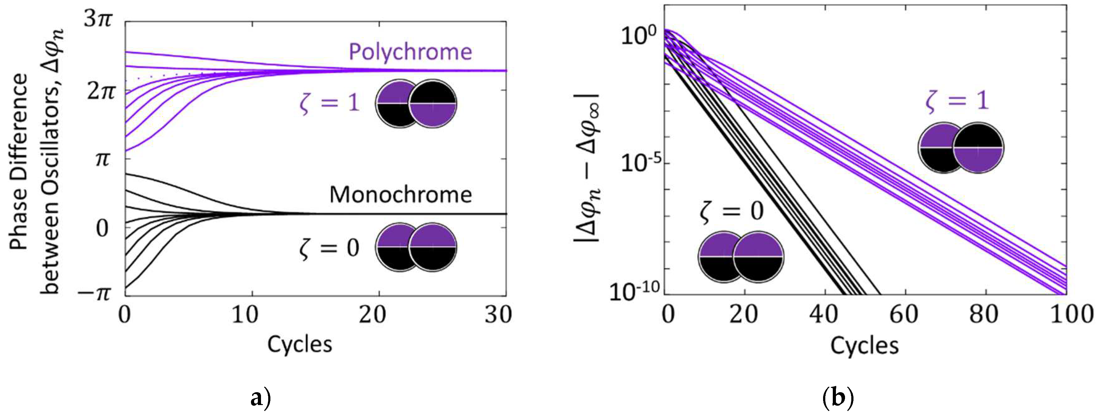
Figure 9.
-profiles for bonds; .
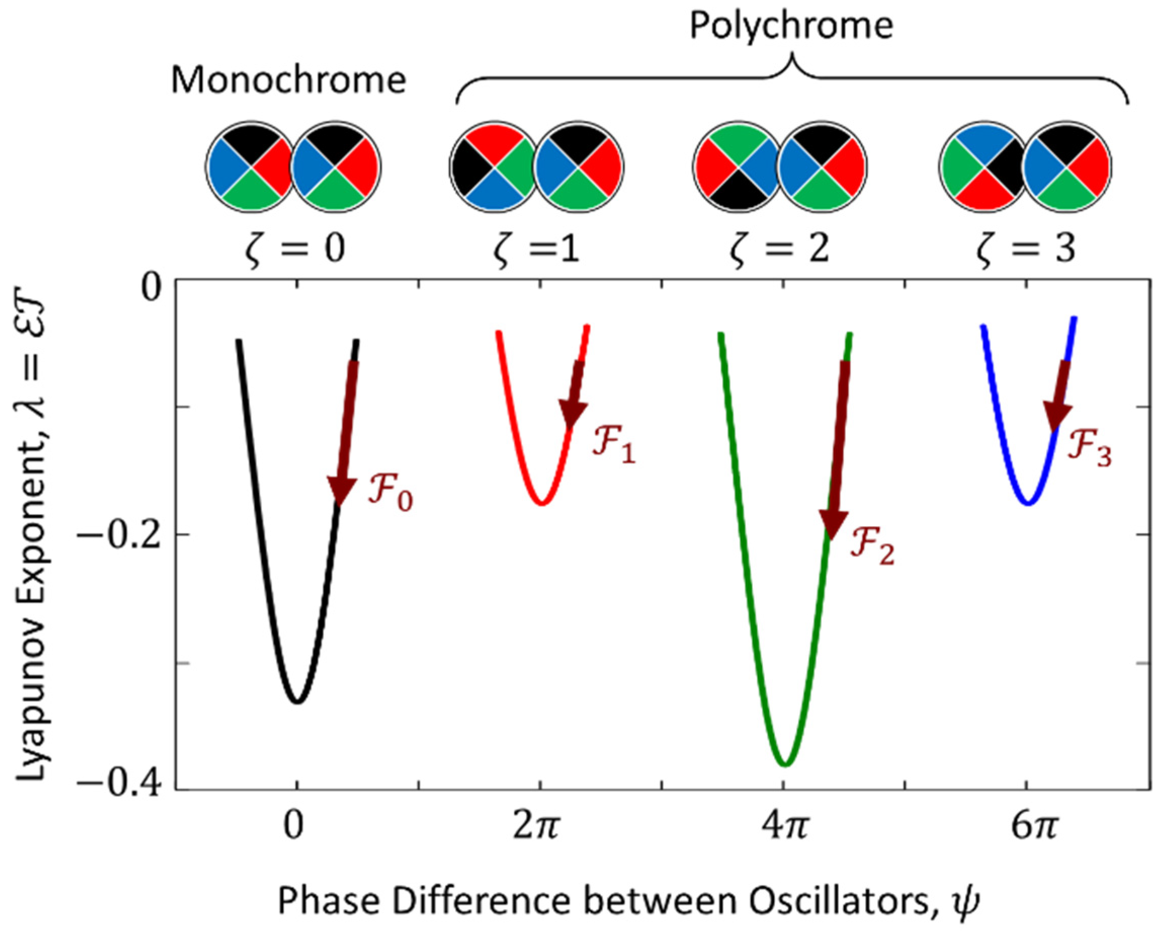
Figure 10.
(a) Network with hypercube topology; (b) a fragment of the network including three edges, each representing a chaos generator; (c) typical generator waveform; (d) correlation functions between resistor nodes.
Figure 10.
(a) Network with hypercube topology; (b) a fragment of the network including three edges, each representing a chaos generator; (c) typical generator waveform; (d) correlation functions between resistor nodes.
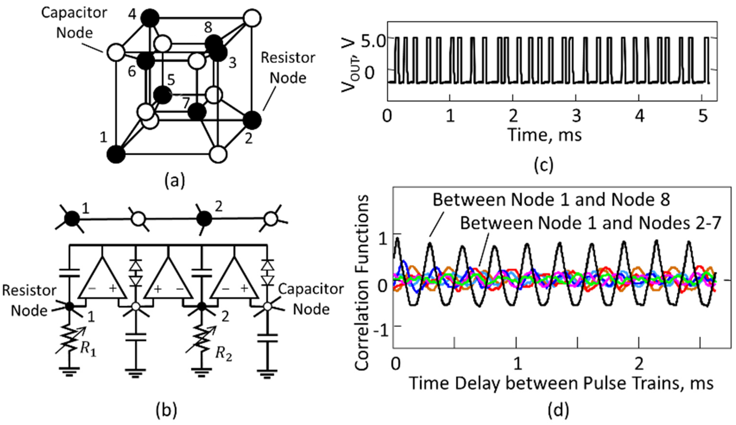
Figure 11.
Tunneling of a spinorial defect: (a) before transfer, (b) during transfer, (c) after relaxation.
Figure 11.
Tunneling of a spinorial defect: (a) before transfer, (b) during transfer, (c) after relaxation.
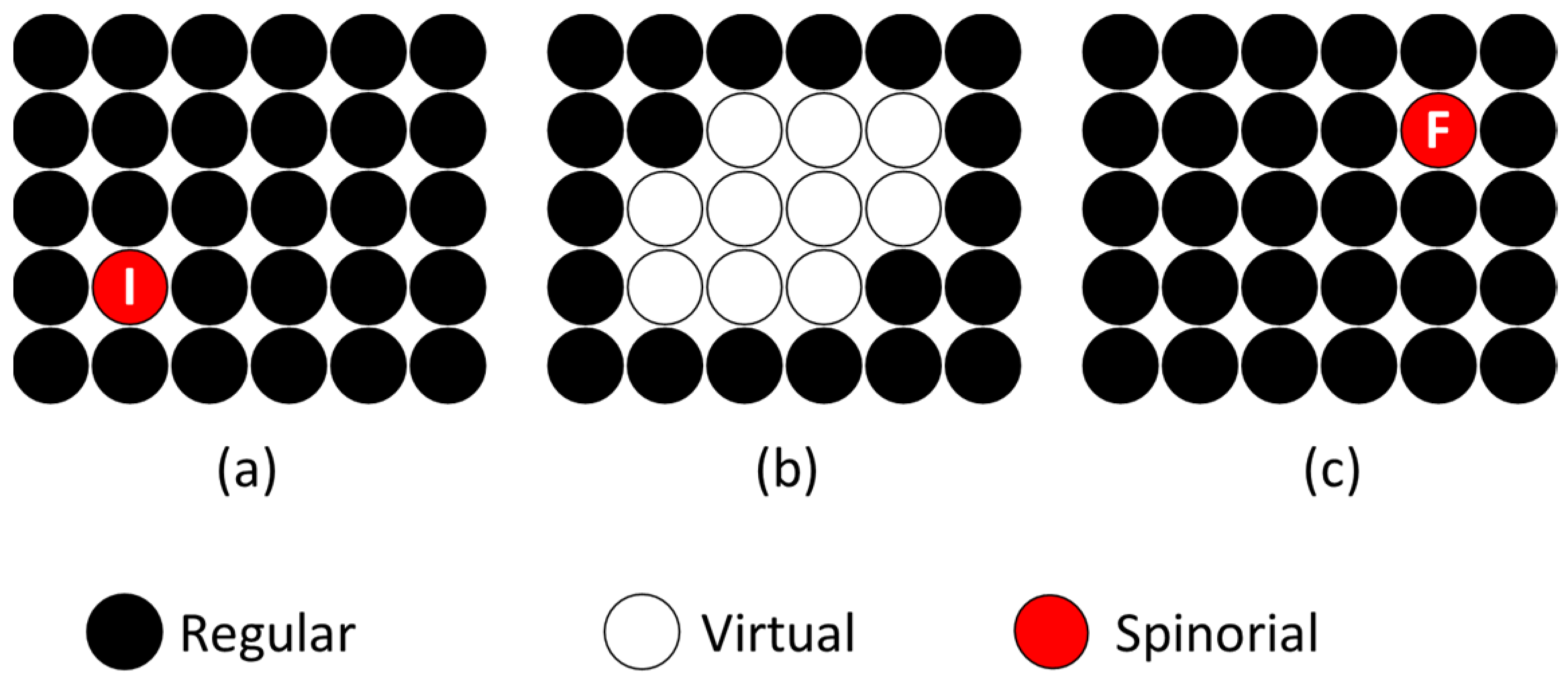
Figure 12.
Entanglement: (a) before excitation, (b) during excitation, (c) after relaxation.
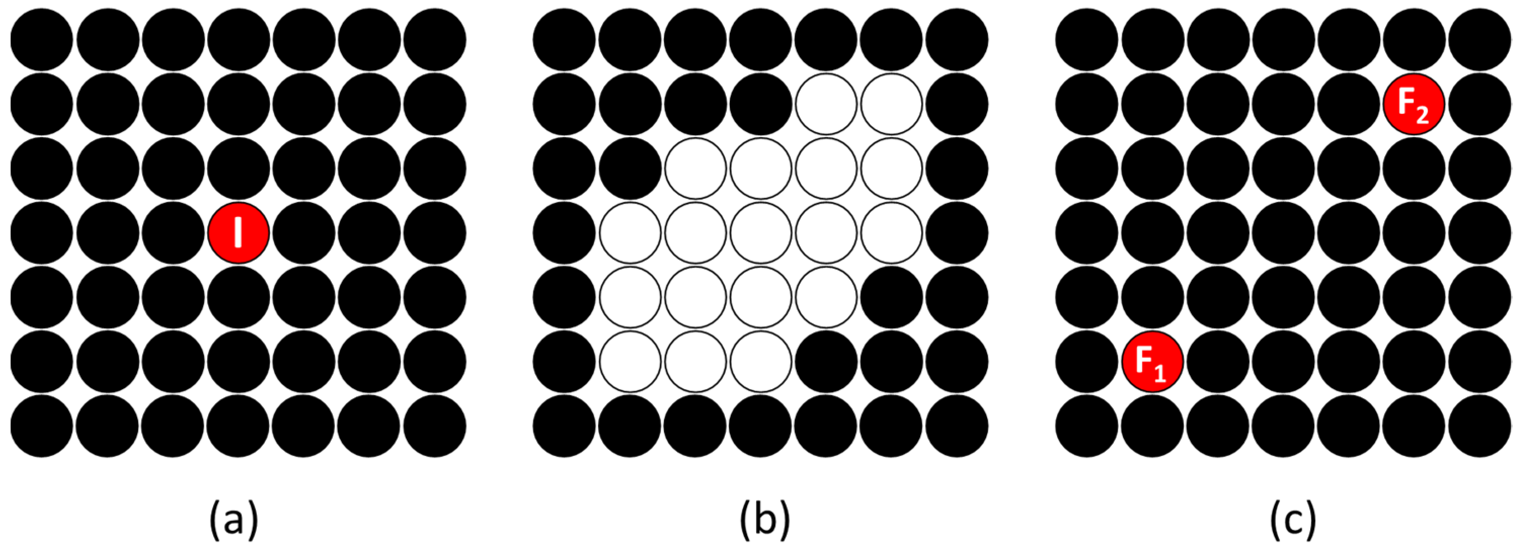
Figure 13.
Spinorial clock diagrams for matter and antimatter vortices in different vacuum phases.
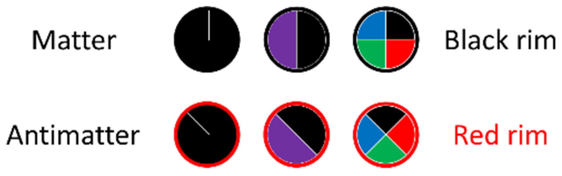
Figure 14.
Topological-phase diagram.
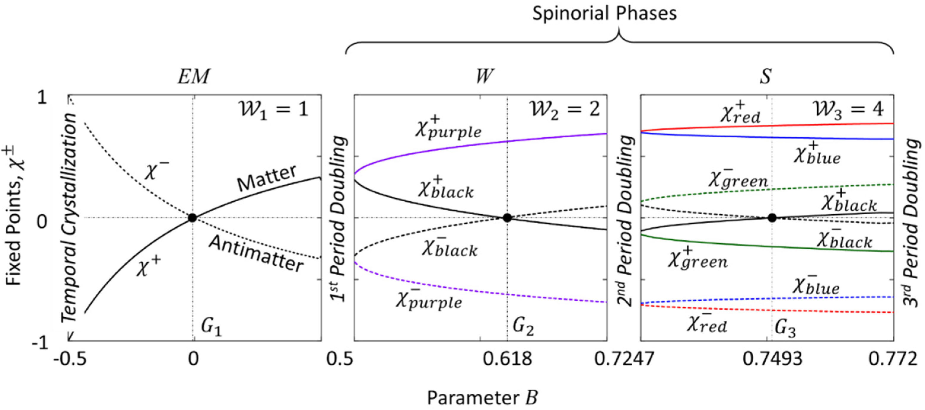
Figure 15.
profile in three vacuum phases.
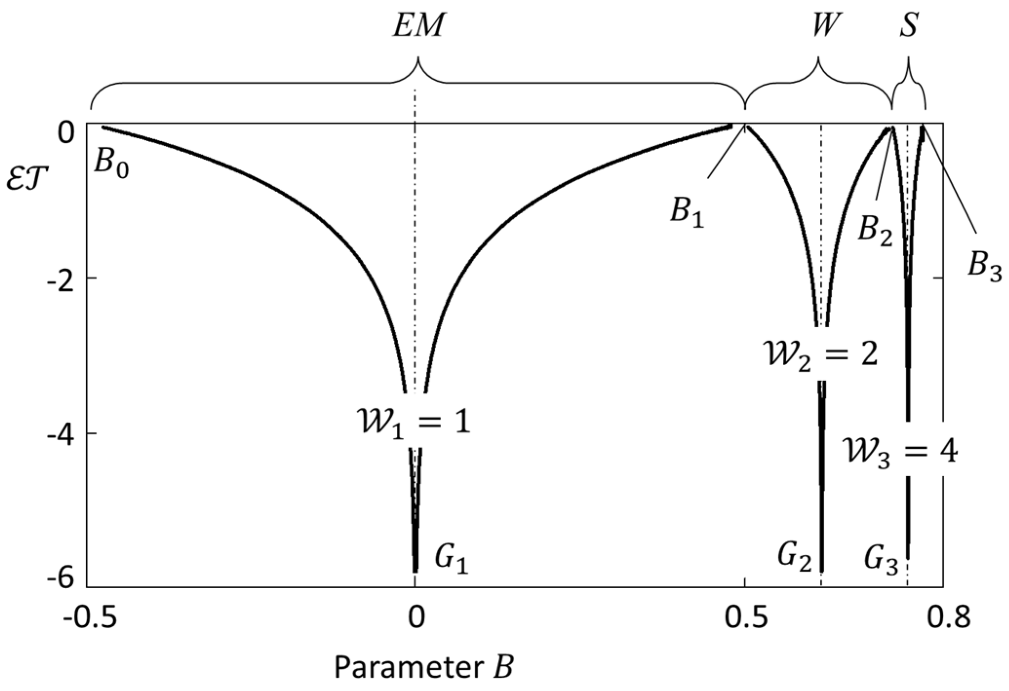
Figure 16.
Distribution of vacuum vortices in different topological phases.
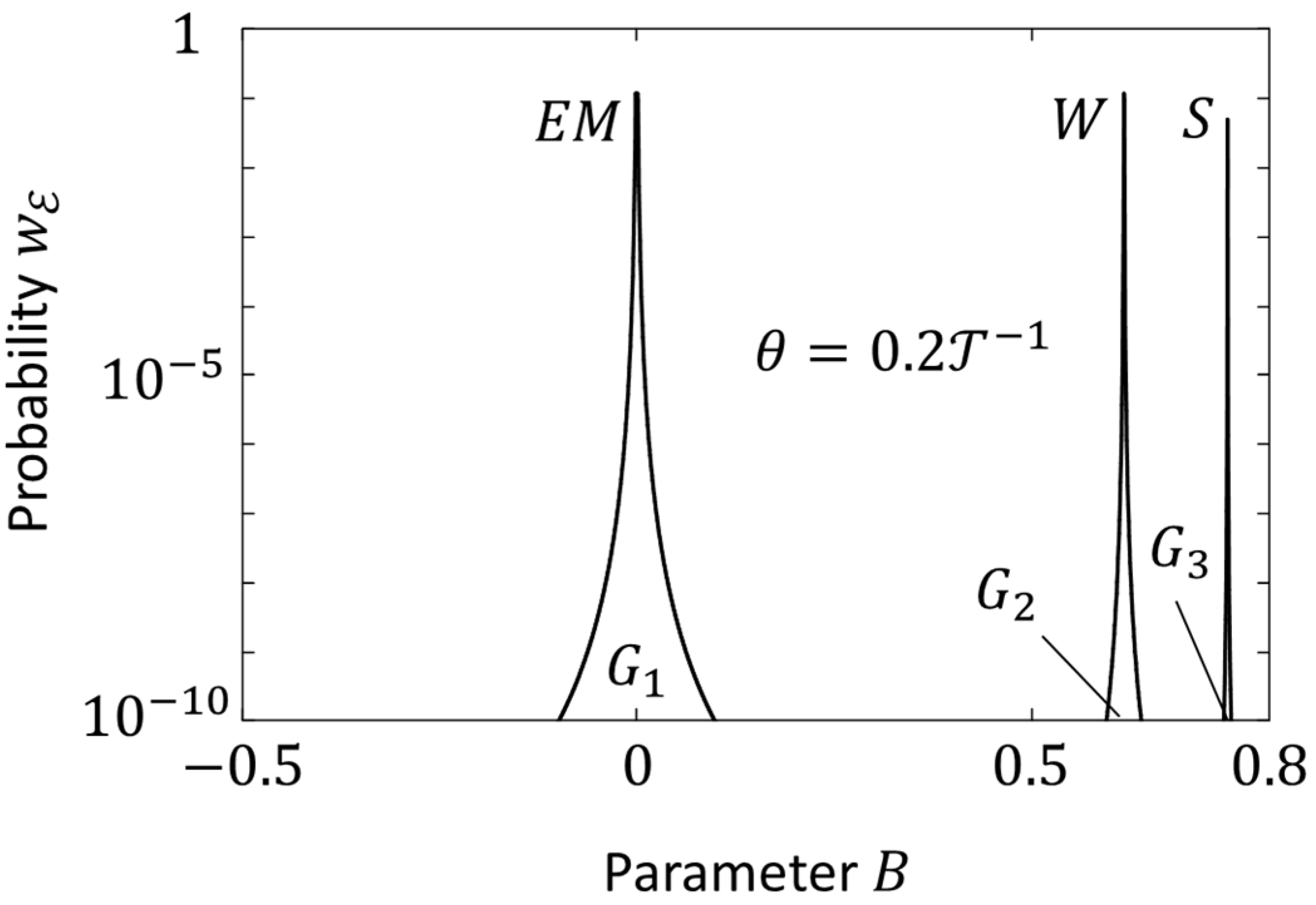
Figure 17.
(a) Half a spinon torus; (b) -spinon flavors, (c) -spinon flavors.
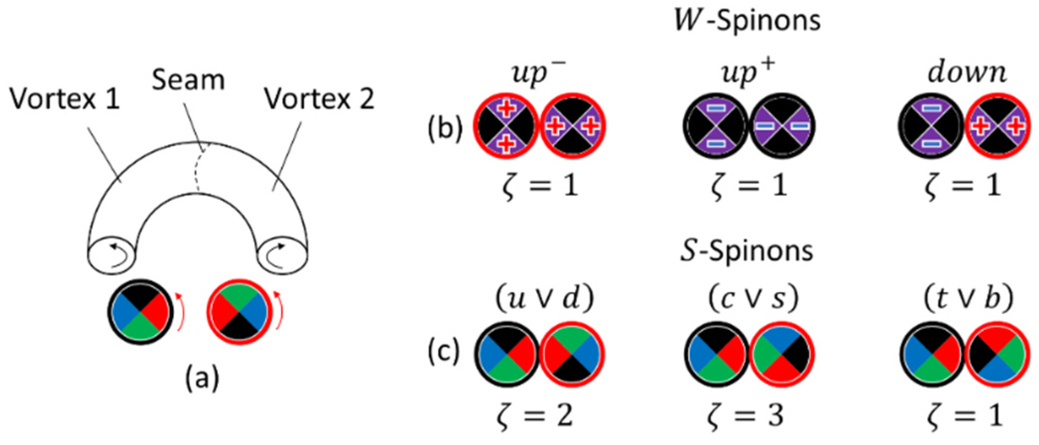
Figure 18.
Example of a flavor change from to .
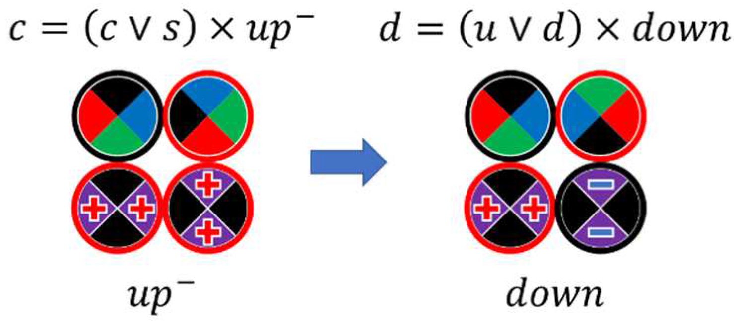
Figure 19.
Three generations of prototype leptons.
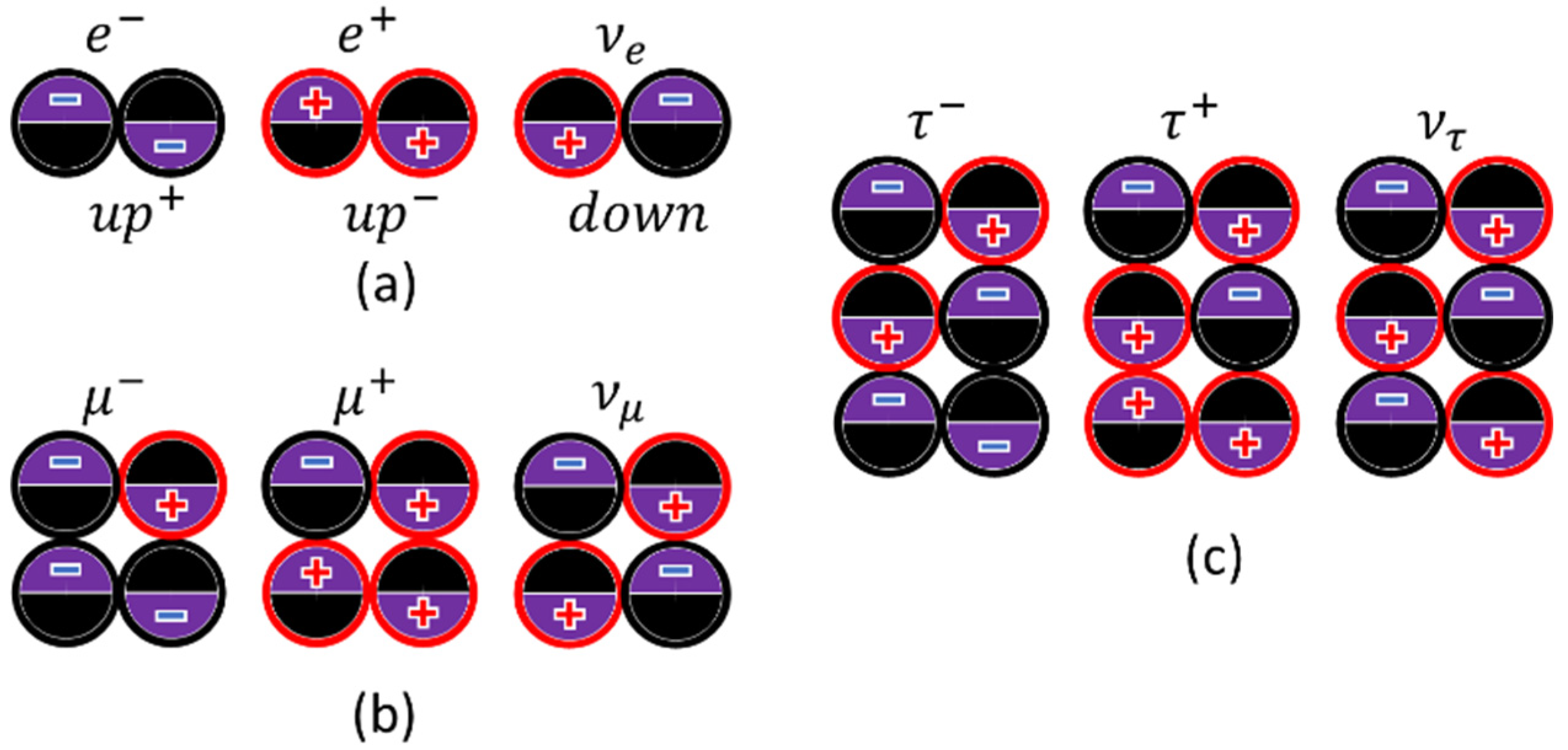
Figure 20.
Spinon representation of “eightfold way” mesons.
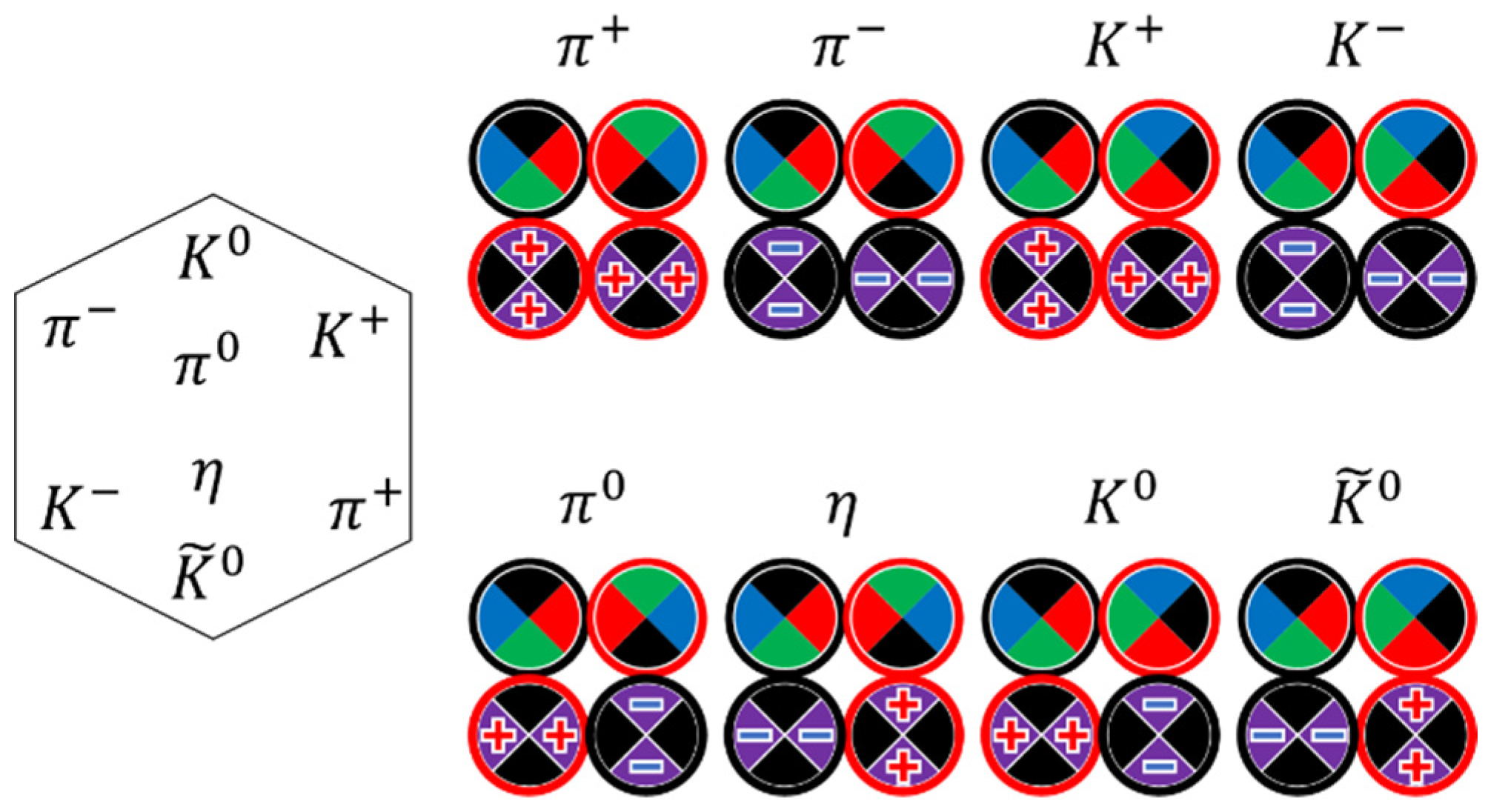
Figure 21.
Spinon representation of “eightfold way” baryons.
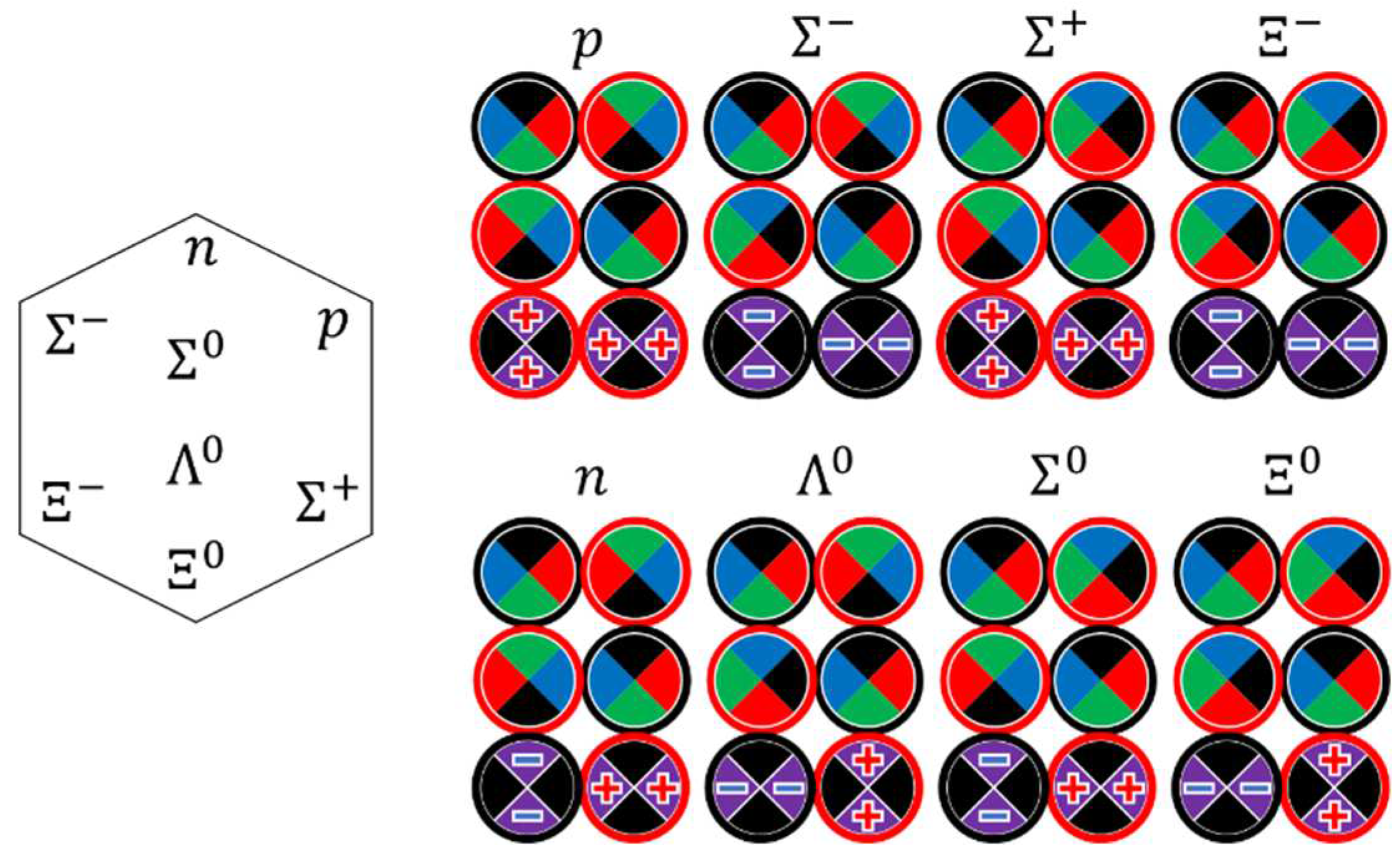
Figure 22.
Flavor rotation diagrams. The excited oscillator is (a) matter; (b) antimatter.
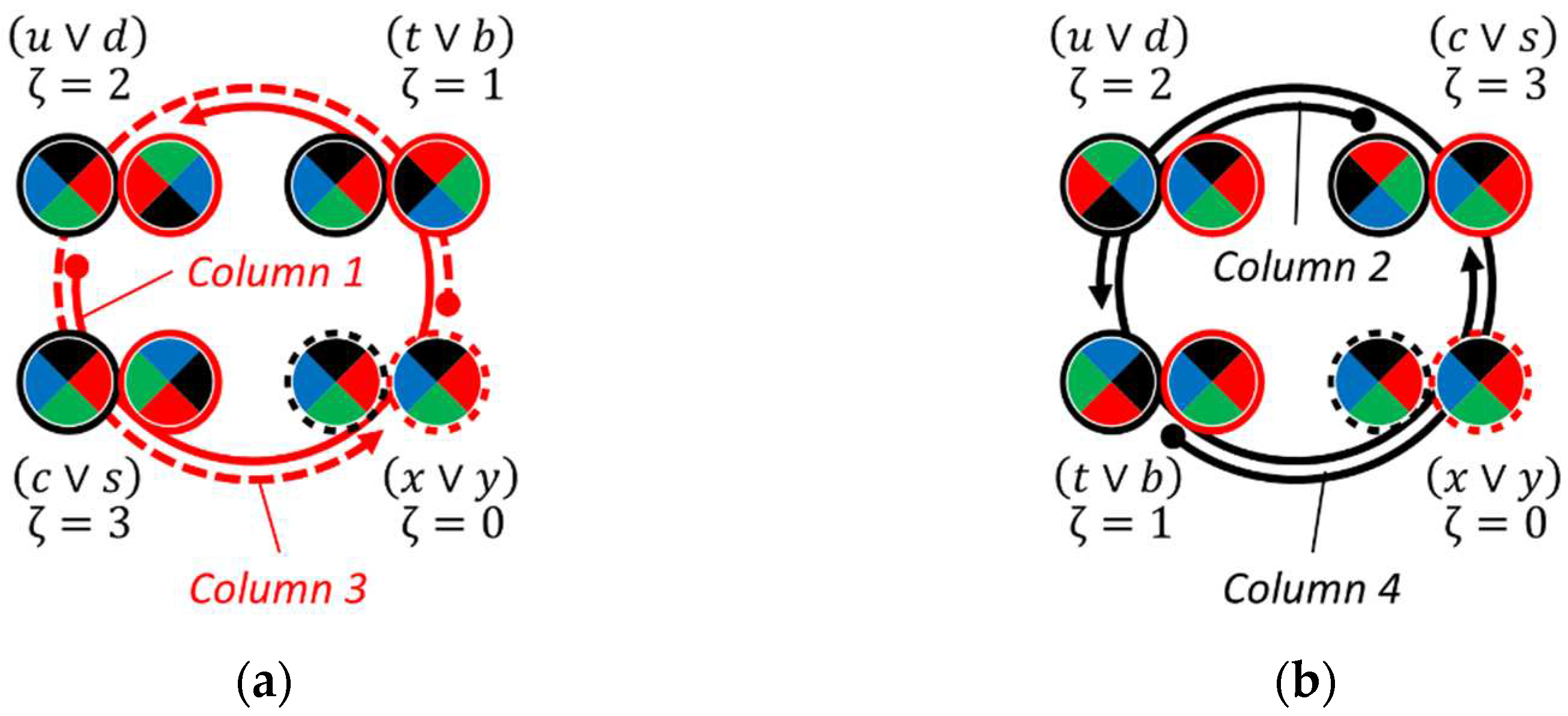

Table 1.
The correspondence chart between the vortex spinorial charges and the standard model boson charges.
Table 1.
The correspondence chart between the vortex spinorial charges and the standard model boson charges.
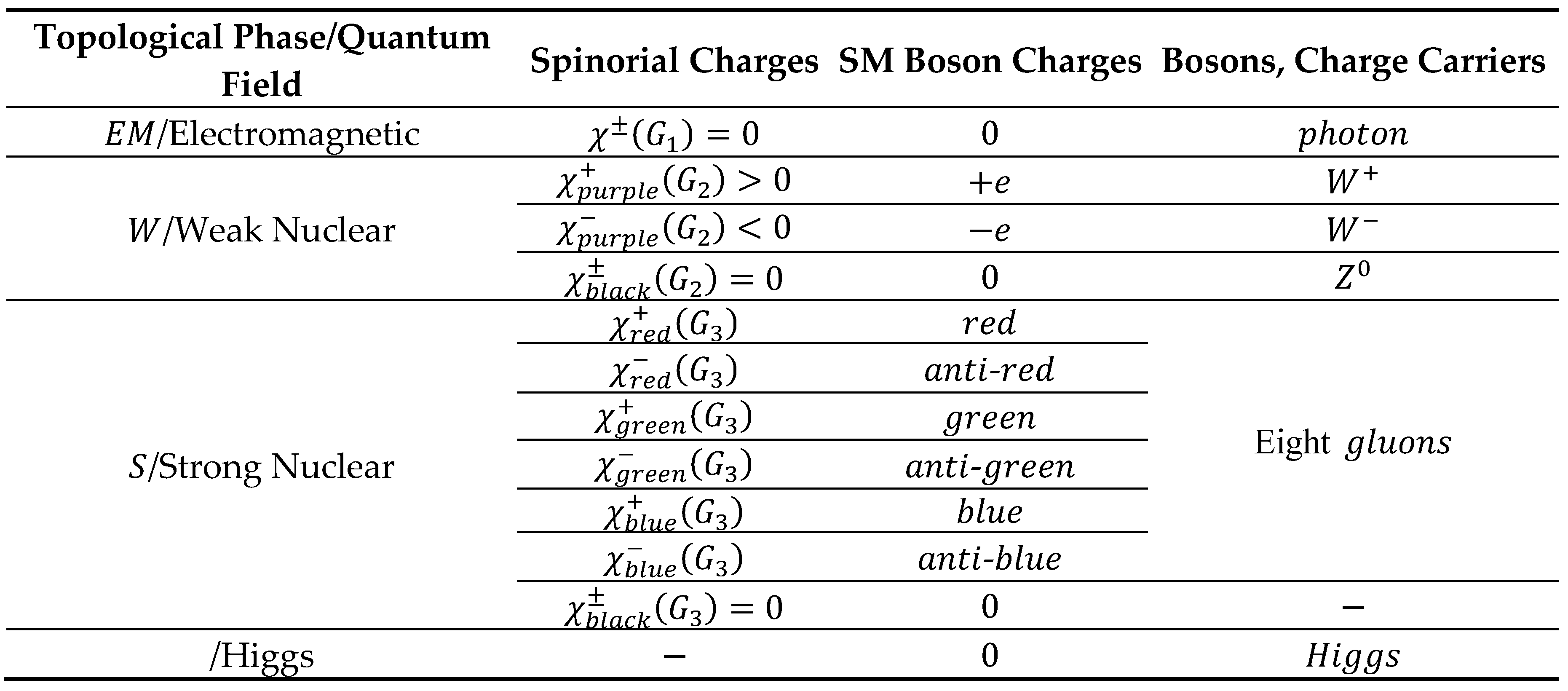 |
Table 2.
Flavor multiplication table.
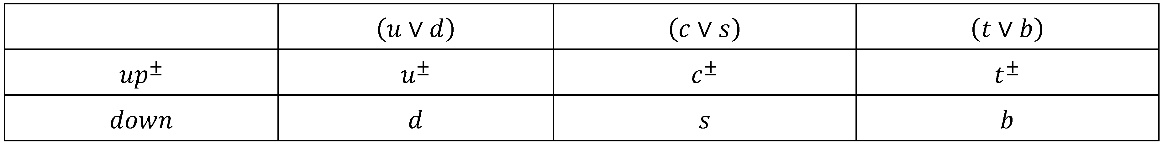 |
Table 3.
Probabilities of flavor change in nonhybridized -spinons.
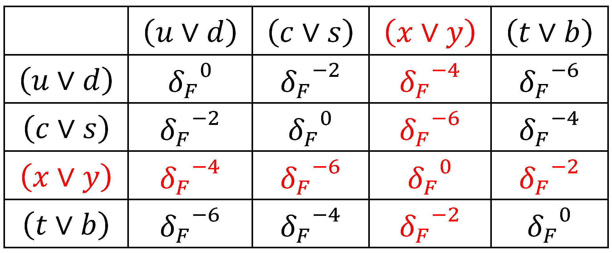 |
Table 4.
(a) Flavor rotation matrix; (b) CKM matrix.
 |
Disclaimer/Publisher’s Note: The statements, opinions and data contained in all publications are solely those of the individual author(s) and contributor(s) and not of MDPI and/or the editor(s). MDPI and/or the editor(s) disclaim responsibility for any injury to people or property resulting from any ideas, methods, instructions or products referred to in the content. |
© 2023 by the authors. Licensee MDPI, Basel, Switzerland. This article is an open access article distributed under the terms and conditions of the Creative Commons Attribution (CC BY) license (http://creativecommons.org/licenses/by/4.0/).
Copyright: This open access article is published under a Creative Commons CC BY 4.0 license, which permit the free download, distribution, and reuse, provided that the author and preprint are cited in any reuse.


