Submitted:
07 May 2025
Posted:
08 May 2025
Read the latest preprint version here
Abstract
In special relativity (SR) and general relativity (GR), there are two concepts of time: coordinate time t and proper time τ. Two facts deserve reflection: (1) Clocks measure τ, but τ is assigned a much smaller role in the equations of physics than t. (2) Cosmologists are aware of the Hubble parameter Hθ, but when parameterizing worldlines in spacetime, the parameter τ is preferred over θ = 1/Hθ. Here we show: There is a different description of nature that does not conflict with SR/GR. Euclidean relativity (ER) uses τ as a coordinate, θ as the “cosmic evolution parameter”, and a Euclidean metric. All energy moves through 4D Euclidean space (ES) at the speed c. The laws of physics have the same form in each object’s reference frame. An object’s reference frame is spanned by its proper space and proper time. Each object experiences its 4D motion as proper time τ, which is the length of a 4D Euclidean vector “flow of proper time” τ. Any acceleration rotates an object’s τ and curves its worldline in flat ES. τ proves crucial for objects that are very far away or entangled. Information hidden in θ and τ is not available in SR/GR. ER solves 15 fundamental mysteries, such as the nature of time, the Hubble tension, the wave–particle duality, and the baryon asymmetry. On top, ER declares cosmic inflation, expanding space, dark energy, and non-locality obsolete.
Keywords:
spacetime
; cosmology
; Hubble tension
; dark energy
; quantum mechanics
; non-locality
There are two approaches to describing nature: either in “empirical concepts” (based on observing) or else in “natural concepts” (inherent in all objects). Observing implies that the description may not be complete or that some of the applied concepts are obsolete. Special and general relativity (SR/GR) take the first approach [1,2], but there is no absolute time in SR/GR and thus no “holistic view” (universal for all objects at the same instant in time). Euclidean relativity (ER) takes the second approach and provides a holistic view. In this paper, I show that natural concepts improve our understanding of nature. For a better readability, I refer to an observer as “he”. To compensate, I refer to nature as “she”.
A new theory of spacetime must either disprove SR/GR or else not conflict with SR/GR. Because of different concepts, ER does not conflict with SR/GR. However, ER tells us that the scope of SR/GR is limited: We must apply ER to objects that are very far away (such as high-redshift supernovae) or entangled (moving in opposite 4D directions at the speed ). In such extreme situations, the 4D vector “flow of proper time” of ER is crucial. ER raises questions: (1) Does ER predict the same relativistic effects as SR/GR? Yes, the Lorentz factor and gravitational time dilation are recovered in ER. (2) What are the benefits of ER? It solves mysteries of cosmology and quantum mechanics (QM). (3) Does ER also make quantitative predictions? Yes, it predicts the 10 percent deviation in the published values of Request to editors/reviewers: (1) Please read carefully. I do not disprove SR/GR. I show that the scope of SR/GR is limited. (2) Do not reject ER without disproving ER. A new theory deserves full consideration unless it can be disproven. (3) Do not apply the concepts of SR/GR to ER. One reviewer argued that spacetime cannot be Euclidean because it is non-Euclidean in SR/GR. According to this logic, Earth cannot orbit the sun because it does not orbit the sun in the geocentric model. (4) Appreciate illustrations. As a geometric theory, ER complies with the stringency of math. (5) Be fair. One paper cannot cover all of physics. Despite some unanswered questions, ER is very promising because it solves 15 mysteries.
1. Introduction
Today’s concepts of space and time were coined by Albert Einstein. In SR, space and time are fused into a flat spacetime described by the Minkowski metric. SR is often presented in Minkowski spacetime [3]. Predicting the lifetime of muons [4] is one example that supports SR. In GR, a curved spacetime is described by the Einstein tensor. The deflection of starlight [5] and the high accuracy of GPS [6] are two examples that support GR. Quantum field theory [7] unifies classical field theory, SR, and QM, but not GR.
In 1969, Newburgh and Phipps [8] pioneered ER. Montanus [9] added a constraint: A pure time interval must be a pure time interval for all observers. According to Montanus [10], this constraint is required to avoid “distant collisions” (without physical contact) and a “character paradox” (confusion of photons, particles, antiparticles). The constraint is obsolete. Whatever is proper time to me, it can be one axis of proper space for you. There are no distant collisions once we take projections into account. There is no character paradox once we take the 4D vector “flow of proper time” (see Sect. 3) into account. Not only the proper time of an antiparticle can flow backward, but also that of a particle (see Sect. 5.15). Montanus verified the precession of Mercury’s perihelion in ER [10] and other effects [11], but he failed to derive Maxwell’s equations because of a wrong sign [10]. Montanus used coordinate time as the parameter. The correct parameter in ER is cosmic time.
Almeida [12] studied geodesics in ER. Gersten [13] showed that the Lorentz transformation is an SO(4) rotation. There is a website about ER: https://euclideanrelativity.com/. Here is why theorists reject ER: (1) Dark energy and non-locality make cosmology and QM work. (2) The SO(4) symmetry in ER seems to exclude waves. (3) Paradoxes seem to arise. This paper marks a turning point. It shows that dark energy and non-locality are obsolete concepts, SO(4) is compatible with waves, and projections avoid paradoxes.
The two postulates of ER: (1) All energy moves through 4D Euclidean space (ES) at the speed of light . (2) The laws of physics have the same form in each object’s reference frame. An object’s reference frame is spanned by its proper space and proper time. Unlike coordinate space and coordinate time in SR, proper space and proper time are assembled to a Euclidean spacetime. My first postulate is stronger than the second SR postulate: is absolute and universal. My second postulate is not limited to inertial frames. The order of the postulates is reversed. Absoluteness comes first. Relativity comes second.
Fig. 1 left illustrates the reference frames of two objects in ES. Each object experiences that axis in which it moves at the speed as its proper time. It experiences the other three axes as its proper space. Proper space and proper time make up its “reality”. There are as many realities as there are objects. Mathematically, ES is 4D Euclidean space, and proper space/proper time are two orthogonal projections from ES. Physically, only three axes of ES are experienced as spatial, one as temporal, and measuring an object’s coordinates is equivalent to projecting it from ES to an observer’s reality. Fig. 1 right illustrates two approaches to describing nature. We must not play SR/GR and ER off against each other. The concepts of SR/GR do not apply to ER, and vice versa. ER solves mysteries that are rooted in ES.
It is instructive to contrast Newton’s physics, Einstein’s physics, and ER. In Newton’s physics, all energy moves through 3D Euclidean space as a function of independent time. There is no speed limit for matter. In Einstein’s physics, all energy moves through a non-Euclidean spacetime. The 3D speed of matter is . In ER, all energy moves through ES. The 4D speed of all energy is . Newton’s physics [14] influenced many philosophers. I am convinced that ER will reform both physics and philosophy.
2. Identifying an Issue in Special and General Relativity
The fourth coordinate in SR is an observer’s coordinate time . In § 1 of SR, Einstein gives an instruction for synchronizing clocks at the points P and Q. At , a light pulse is sent from P to Q. At , it is reflected at Q. At , it is back at P. The clocks synchronize if
In § 3 of SR, Einstein derives the Lorentz transformation. The coordinates of an event in a system K are transformed to the coordinates in K’ by
where K’ moves relative to K in at the constant speed and is the Lorentz factor. Mathematically, Eqs. (2a–c) are correct: They transform the coordinates from K to K’. There are covariant equations that transform the coordinates from K’ to K. Physically, there is an issue in SR and also in GR: The empirical concepts of SR/GR fail to solve fundamental mysteries. There are coordinate-free formulations of both SR and GR [15,16], but there is no absolute time in SR/GR and thus no “holistic view” (I repeat the important definition: universal for all objects at the same instant in time). The view in SR/GR is “multi-egocentric”: SR/GR work for all observers, but each observer’s view is egocentric. All observers’ views taken together do not make a holistic view because they still do not provide absolute time. Without absolute time, observers will not always agree on what is past and what is future. Physics paid a high price for dismissing absolute time: ER restores absolute time (see Sect. 3) and solves 15 mysteries (see Sect. 5). Thus, the issue is real.
The issue in SR/GR is not about making wrong predictions. It has much in common with the issue in the geocentric model: In either case, there is no holistic view. Geocentrism is the egocentric view of mankind. In the old days, it was natural to believe that all celestial bodies would orbit Earth. Only astronomers wondered about the retrograde loops of some planets and claimed that Earth orbits the sun. In modern times, engineers have improved rulers and clocks. Today, it is natural to believe that it would be fine to describe nature as accurately as possible, but in the empirical concepts of one or more observers. The human brain is smart, but it often takes itself as the center/measure of everything.
The analogy of the geocentric model to SR/GR is not perfect: Heliocentrism and geocentrism exclude each other. ER does not conflict with SR/GR. Nevertheless, the analogy is close: (1) After taking some other planet as the center of the Universe (or after a transformation in SR/GR), the view is still geocentric (or else egocentric). (2) Retrograde loops are obsolete in heliocentrism, but they make geocentrism work. Dark energy and non-locality are obsolete in ER, but they make cosmology and QM work. (3) Heliocentrism overcomes the limited perspective from Earth. ER overcomes the limited perspectives of observing. (4) The geocentric model was a dogma in the old days. SR and GR are dogmata nowadays. Have physicists not learned from history? Does history repeat itself?
3. The Physics of Euclidean Relativity
ER cannot be derived from measurement instructions because the proper coordinates of other objects cannot be measured. We start with the Minkowski metric of SR
where is an infinitesimal distance in proper time , whereas all () and are infinitesimal distances in an observer’s coordinate space and coordinate time . Coordinate spacetime is an empirical spacetime because its coordinates are construed by an observer and thus not inherent in rulers and clocks. Rulers measure proper length. Clocks measure proper time. We introduce ER by its metric
where is an infinitesimal distance in the parameter , whereas all () and are infinitesimal distances in an object’s (!) proper space and proper time . Observers are objects too. The fourth coordinate is . The invariant is . The metric tensor is the identity matrix. I prefer the indices 1–4 to 0–3 to stress the SO(4) symmetry. An object’s proper space and proper time span its reference frame in 4D Euclidean space (ES), where . The orientation of its reference frame in absolute ES can change. ES is experienced as a Euclidean spacetime (EST). EST is a natural spacetime because its coordinates are measured by and thus inherent in rulers and clocks. Intrinsic rulers and clocks of all objects measure distances in EST and not in coordinate spacetime! Do not confuse ER with a Wick rotation [17], which keeps invariant.
Montanus [9] distinguished “absolute Euclidean spacetime” (AEST) from a “relative Euclidean spacetime” (REST). His AEST is my ES. His REST is my EST. Montanus [9,10,11] promoted AEST, but he unnecessarily disqualified REST. He rejected the idea of four fully symmetric axes. I show: Whatever is proper time to me, it can be one axis of proper space (or a mix of proper space and proper time) for you. Montanus merely rearranged Eq. (3) to make the metric look Euclidean. He did not distinguish between and .
Each object is free to label the axes of its reference frame. We assume: It labels the axis of its current 4D motion as . Because of my first postulate, it thus always moves in the axis at the speed . If the object moves along a curved worldline in ES, the orientation of its reference frame always adapts to the curvature as if the frame were gimbal-mounted to the origin of ES. Because of length contraction at the speed (see Sect. 4), the axis disappears for itself and is experienced as proper time. Objects moving in the axis at the speed experience the axis as proper time. Each object experiences its 4D motion as proper time , which is the length of a 4D Euclidean vector “flow of proper time” . Information hidden in and is not available in SR/GR.
where is an object’s 4D velocity. In ER, speed is not defined as (), but as (). Thus, Eq. (4) is nothing but my first postulate
Because of , there is no continuous transition between Eqs. (3) and (4) nor between SR/GR and ER. This fact underlines that ER provides a unique description of nature. SR describes nature in empirical concepts , where is some object-related parameter. GR is locally equivalent to SR. ER describes nature in natural concepts , where is what I call the “cosmic evolution parameter”. When parameterizing worldlines in spacetime, the parameter proves more powerful than . Only in proper coordinates can we access ES, but the proper coordinates of other objects cannot be measured. In my Conclusions, I will explain why this is fine.
It is instructive to contrast three concepts of time. is a subjective measure of time: An observer uses his clock as the master clock. is an objective measure of time: Clocks measure independently of observers. is the total distance covered in ES (length of a worldline) divided by . As the invariant in Eq. (4), is a concept of absolute time. This is why I also call it “cosmic time”. By referring to , observers can agree on what is past and what is future. Regarding causality, a finite is incompatible with a coordinate “absolute time”. However, it is compatible with a parameter “absolute time”.
We consider two identical clocks “r” (red clock) and “b” (blue clock). In SR, “r” moves in the axis. Clock “b” starts at and moves in the axis at a constant speed of . Fig. 2 left shows the instant when either clock moved 1.0 Ls (light seconds) in . Clock “b” moved 0.6 Ls in and 0.8 Ls in . It displays “0.8”. In ER, “r” moves in the axis. Fig. 2 right shows the instant when either clock moved 1.0 s in its proper time. Both clocks display “1.0”. Since “r” remains at and “b” remains at , there is for “r” and for “b” according to Eq. (4). A uniformly moving clock always displays both its and . However, is not invariant in ER. Thus, of “r” is not equal to of “b”. In ER, is invariant. Thus, of “r” is equal to of “b”.
We now assume that an observer R (or B) moves with clock “r” (or else “b”). In SR and only from the perspective of R, clock “b” is at when “r” is at (see Fig. 2 left). Thus, “b” is slow with respect to “r” in (of B). In ER and independently of observers, clock “b” is at when “r” is at (see Fig. 2 right). Thus, “b” is slow with respect to “r” in (of R). In SR and ER, “b” is slow with respect to “r”, but time dilation occurs in different axes. Experiments do not disclose that axis in which a clock is slow. Thus, both SR and ER describe time dilation correctly if ER yields the same Lorentz factor as SR. In Sect. 4, I will show that this is the case.
Note that the Michelson–Morley experiment [18] refutes a 3D ether, but not absolute ES and its projections to an object’s proper space and proper time. Note also that “relativity” has different connotations in SR and ER. In SR, spatial/temporal distances are relative: They depend on an observer’s frame of reference. In ES, there are no spatial/temporal distances. All are “pure distances”. Only objects/observers experience three axes of ES as spatial and one as temporal. However, the orientation of a frame of reference in ES is relative: It depends on an object’s/observer’s 4D vector . There is also a difference regarding clock synchronization: In SR, R synchronizes clock “b” to his clock “r” (same value of in Fig. 2 left). If he does, the clocks are not synchronized for B. In ER and independently of observers, clocks with the same are naturally synchronized, while clocks with different and are never synchronized (different values of in Fig. 2 right).
But why does ER provide a holistic view? Eq. (4) is symmetric in all (). R and B experience different axes as temporal. This is why Fig. 2 left works for R, but not for B: A second Minkowski diagram is required, where and are orthogonal. Here the view is multi-egocentric. In contrast, Fig. 2 right works for R and for B at once (at the same cosmic time): Not only are and orthogonal, but also and . ES is independent of observers and thus absolute. Here the view is universal and thus holistic.
Regarding waves, I was misled by editors who insisted that the SO(4) symmetry of ES is incompatible with waves. SO(4) is incompatible with waves that propagate as a function of a coordinate time , but compatible with waves that propagate as a function of the cosmic evolution parameter . This is because Eq. (4) can be rewritten as
which is of the same form as Eq. (3). A big advantage of mathematics is that it remains the same when we replace the variables. Maxwell’s equations thus have the same form in ER as in today’s physics except that replaces and waves can propagate in one out of four axes. I claim: All objects are “wavematters” (pure energy) that propagate through and oscillate in ES as a function of the parameter . I will give evidence of my claim in Sect. 5.13.
4. Geometric Effects in Euclidean Relativity
We consider two identical rockets “r” (red rocket) and “b” (blue rocket). Let observer R (or B) be in the rear end of “r” (or else “b”). The 3D space of R (or B) is spanned by (or else ). We use “3D space” as a synonym of proper space. The proper time of R (or B) relates to (or else ) according to Eq. (5). Both rockets start at the same point P and at the same cosmic time . They move relative to each other at the constant speed . R and B are free to label the axis of relative motion in 3D space. R (or B) labels it as (or else ). The ES diagrams in Fig. 3 must fulfill my two postulates and the initial conditions (same P, same ). This is achieved by rotating the red and the blue frame with respect to each other. Do not confuse ES diagrams with Minkowski diagrams. In ES diagrams, objects maintain proper length and clocks display proper time. For a better readability, a rocket’s width is drawn in (or ), although its width is in (or else ).
Up next, we verify: Projecting distances in ES to the axes and of an observer causes length contraction and time dilation. Let (or ) be the length of rocket “b” for observer R (or else B). In a first step, we project “b” in Fig. 3 left to the axis.
where is the same Lorentz factor as in SR. For observer R, rocket “b” contracts to . Despite the Euclidean metric, we calculate the same Lorentz factor as in SR. We now ask: Which distances will R observe in the axis? We rotate rocket “b” until it serves as a ruler for R in the axis. In his 3D space, this ruler contracts to zero length. In other words: The axis disappears for R because of length contraction at the speed . In a second step, we project “b” in Fig. 3 left to the axis.
where (or ) is the distance that B moved in (or else ). With (R and B cover the same distance in ES, but in different 4D directions), we calculate
where is the distance that R moved in . Eqs. (9) and (12) tell us: is recovered in ER if we project ES to the axes and of an observer. This result is significant: It tells us that ER predicts the same relativistic effects as SR. The rockets serve as an example. Other objects are projected the same way. For orthogonal projections, the reader is referred to geometry textbooks [19,20]. For instance, and the lifetime of a muon are recovered in ER when R is kept as the observer and the blue rocket is replaced by a muon.
We now transform the proper coordinates of observer R (unprimed) to the ones of B (primed). R cannot measure the proper coordinates of B, and vice versa, but we can always calculate them from ES diagrams. Fig. 3 right tells us how to calculate the 4D motion of R in the proper coordinates of B. The transformation is a 4D rotation by the angle .
Up next, I show that not only the Lorentz factor is recovered in ER, but also gravitational time dilation. Clock “r” and Earth move in the axis at the speed (see Fig. 4). Clock “b” accelerates toward Earth while maintaining the speed in ES. Because of Eq. (7), there are only transversal accelerations in ES. The speed of “b” in increases at the expense of its speed in . Thus, “b” is slow with respect to “r” in .
Initially, our two clocks shall be very far away from Earth. Eventually, clock “b” falls freely toward Earth. The kinetic energy of “b” (mass ) in the axis of “r” is
where is the gravitational constant, is the mass of Earth, and is the distance of “b” to Earth in the 3D space of “r”. By applying Eq. (7), we get
With (“b” moves in the axis at the speed ) and (“r” moves in the axis at the speed ), we calculate
where is the same dilation factor as in GR. Eq. (17) tells us: is recovered in ER if we project ES to the axis of an observer. This result is significant: It tells us that ER predicts the same gravitational time dilation as GR. However, curved spacetime in GR replaces gravitational fields. In ER, gravitational fields celebrate a comeback. Any acceleration rotates an object’s and curves its worldline in flat ES.
Clock “b” is slow with respect to “r” in . Since “r” displays both its and , “b” is slow even with respect to , although is absolute time. An accelerated clock displays its , but not . For this reason, clocks placed next to each other display different times after being exposed to different gravitational fields. Since does not depend on , “b” is slow with respect to whether or not it keeps on moving relative to Earth. Action at a distance is not an issue if variations in field strength also spread at the speed . I invite theorists to show: (1) Gravitational waves [21] are compatible with ER. (2) Variational principles [22] are an alternative to derive ER. I showed that and are recovered in ER.
Summary of time dilation: In SR, a uniformly moving clock “b” is slow with respect to “r” in the time axis of “b”. In GR, an accelerated clock “b” or else a clock “b” in a more curved spacetime is slow with respect to “r” in the time axis of “b”. In ER, a clock “b” is slow with respect to “r” in the time axis of “r” (!) if the 4D vector of “b” differs from the 4D vector of “r”. Since both and are recovered in ER, the Hafele–Keating experiment [23] supports ER too. GPS works in ER just as well as in SR/GR.
Fig. 5 illustrates how to read ES diagrams. Problem 1: Two objects move through ES. “r” moves in . “b” emits a radio signal at . The signal recedes radially from “b” in all axes as a function of , but cannot catch up with “r” in the axis. Can the signal and “r” collide in the 3D space of “r” if they do not collide in ES? Problem 2: A rocket moves along a guide wire. The wire moves in . The rocket’s speed in is less than . Doesn’t the wire escape from the rocket? Problem 3: Earth orbits the sun. The sun moves in . Earth’s speed in is less than . Doesn’t the sun escape from Earth’s orbit?
The last paragraph seems to reveal paradoxes in ER. The fallacy lies in the assumption that all four axes would be spatial at once. This is not the case. Only three axes of ES are experienced as spatial and one as temporal. We solve all problems by projecting ES to the 3D space of that object which moves in at the speed . In its 3D space, it is always at rest. The radio signal collides with “r” in the 3D space of “r” if () at one instant in cosmic time . Thus, a collision is possible even if there is . Two objects collide when their positions in coincide. In Fig. 5 left, the signal collides with “r” once has elapsed since “r” started from the origin. Collisions in 3D space do not show up as collisions in ES. In ER, events are not a function of , but a function of the parameter . This parameter is not an axis in ES diagrams. ES diagrams do not show events, but each object’s flow of proper time. The sun does not spatially escape from Earth’s orbit. Rather, the sun and Earth are aging in different 4D directions.
5. Outlining the Solutions to 15 Fundamental Mysteries
In Sect. 5.1 through 5.15, ER solves 15 mysteries and declares four concepts obsolete.
5.1. The Nature of Time
Clocks measure proper time . This fact is true even under acceleration. Cosmic time is the total distance covered in ES divided by . A uniformly moving clock always displays both its and . An accelerated clock displays its , but not . An observed clock’s 4D vector can differ from the observer’s 4D vector . If it does, the observed clock is slow with respect to the observer’s clock in his time axis.
5.2. Time’s Arrow
“Time’s arrow” is a synonym of time flowing forward only. Why does time flow forward only? Here is the answer: Covered distance cannot decrease, but only increase.
5.3. The Factor
in the Energy Term
In SR, the total energy of an object (mass ) in the absence of forces is given by
where is its kinetic energy in an observer’s coordinate space and is its energy at rest. The term can be derived from SR, but SR does not tell us why there is a factor in the energy of objects that move at a speed less than . ER is eye-opening: An object is never “at rest”. From its perspective, is zero and is its kinetic energy in . The factor is a hint that it moves through ES at the speed . In SR, there is also
where is the total momentum of an object and is its momentum in an observer’s coordinate space. Again, ER is eye-opening: From its perspective, is zero and is its momentum in . The factor is a hint that it moves through ES at the speed .
5.4. Length Contraction and Time Dilation
In SR, length contraction and time dilation can be traced back to Einstein’s instruction for synchronizing clocks. In ER, these relativistic effects are natural effects: They stem from projecting distances in ES to the axes and of an observer.
5.5. Gravitational Time Dilation
In GR, gravitational time dilation stems from curved spacetime. In ER, this relativistic effect stems from projecting curved worldlines in ES to the axis of an observer. Eq. (7) tells us: If an object accelerates in his proper space, it automatically decelerates in his proper time. More studies are required to understand other gravitational effects in ER.
5.6. The Cosmic Microwave Background (CMB)
In the inflationary Lambda-CDM model, the Big Bang occurred “everywhere” (space inflated from a singularity). In Sect. 5.6 through 5.12, I outline an ER-based model of cosmology, in which the Big Bang can be localized: It injected a huge amount of energy into ES at an origin O. Cosmic time is the total time that has elapsed since the Big Bang. At , all energy started moving radially away from O. The Big Bang was a singularity in providing energy and radial momentum. Ever since the Big Bang, this energy has been moving through ES at the speed . Shortly after , energy was highly concentrated. While it became less concentrated, plasma particles were created in the projection to any 3D space. Recombination radiation was emitted that we still observe as CMB today [24].
The ER-based model must be able to answer these questions: (1) Why is the CMB so isotropic? (2) Why is the temperature of the CMB so low? (3) Why do we still observe the CMB today? Here are some possible answers: (1) The CMB is so isotropic because it has been scattered equally in the 3D space of Earth. (2) The temperature of the CMB is so low because the plasma particles receded at a very high speed (Doppler redshift, see Sect. 5.11). (3) We still observe the CMB today because the radiation reaches Earth after having covered the same distance in (multiple scattering) as Earth in .
5.7. The Hubble–Lemaître Law
Earth and a galaxy G recede from the origin O of ES at the speed (see Fig. 6 left). While doing so, G recedes from the axis at the speed . Distance (or ) is the distance of G to Earth in the 3D space of Earth at the time (or else ). Because of the 4D Euclidean geometry, relates to as relates to the radius of an expanding 4D hypersphere. All energy is within this hypersphere. Some energy is in its 3D hypersurface. The 4D motion of energy can change continuously by a transversal acceleration (scattering, gravitational field) or discontinuously (photon emission, pair production).
where is the Hubble parameter. If we observe G today at the cosmic time , the recession speed and remain unchanged. Thus, Eq. (20) turns into
where is the Hubble constant, , and is today’s radius of the 4D hypersphere. Eq. (21) is an improved Hubble–Lemaître law [25,26]. Cosmologists are aware of and . They are not yet aware that the 4D geometry is Euclidean, that is absolute, and that is equal to (not to ). Out of two galaxies, the one farther away recedes faster, but each galaxy maintains its recession speed . Time dilation results from Eq. (7): Since G moves in at the speed , it moves in at the speed . Thus, a clock in G is slow with respect to a clock on Earth in the axis and by the factor . The values of Earth and an energy (emitted by G at the time ) never match. Can and Earth collide in the 3D space of Earth if they do not collide in ES? As in Fig. 5 left, collisions in 3D space do not show up as collisions in ES. collides with Earth once has covered the same distance in as Earth in .
5.8. The Flat Universe
Two orthogonal projections from flat ES make up an observer’s reality. This is why he experiences two independent structures: flat 3D space and time.
5.9. Cosmic Inflation
Most cosmologists [27,28] believe that an inflation of space shortly after the Big Bang explains the isotropic CMB, the flat universe, and large-scale structures. The latter inflated from quantum fluctuations. I just showed that ER explains the first two effects. ER even explains large-scale structures if the impacts of quantum fluctuations have been expanding like the 3D hypersurface. In ER, cosmic inflation is an obsolete concept.
5.10. Cosmic Homogeneity (Horizon Problem)
How can the universe be so homogeneous if there are causally disconnected regions? In the Lambda-CDM model, region A at and region B at are causally disconnected unless we postulate cosmic inflation. Without inflation, information could not have covered since the Big Bang. The ER-based model applies natural concepts: Region A is at (see Fig. 6 left). Region B is at (not shown in Fig. 6 left). For A and for B, their axis (equal to Earth’s axis) disappears because of length contraction at the speed . Since A and B overlap spatially in their 3D space, they are causally connected. Note that their opposite 4D vectors “flow of proper time” do not affect causal connectivity as long as A and B overlap spatially.
5.11. The Hubble Tension
Up next, I show that ER predicts the 10 percent deviation in the published values of (known as the “Hubble tension”). We consider CMB measurements and distance ladder measurements. According to team A [29], there is . According to team B [30], there is . Team B made efforts to minimize the error margins in the distance measurements, but there is a systematic error in team B’s value of . The error stems from assuming a wrong cause of the redshifts.
We assume that team A’s value of is correct. We simulate the supernova of a star S that occurred at a distance of from Earth (see Fig. 6 right). The recession speed of S is calculated from measured redshifts. The redshift parameter tells us how each wavelength of the supernova’s light is either stretched by an expanding space (team B) or else Doppler-redshifted by receding objects (ER-based model). The supernova occurred at the cosmic time , but we observe it today at the cosmic time (see Fig. 6 right). While the supernova’s light moved the distance in the axis, Earth moved the same distance , but in the axis (first postulate). There is
For a short distance of , Eq. (22) tells us that deviates from by only 0.009 percent. When plotting versus for distances from 0 Mpc to 500 Mpc in steps of 25 Mpc (red points in Fig. 7), the slope of a straight-line fit through the origin is roughly 10 percent greater than . Since team B calculates from versus magnitude, which is like plotting versus , its value of is roughly 10 percent too high. Team B’s value of is not correct because Eq. (21) tells us: We must plot versus to get a straight line (blue points in Fig. 7). Ignoring the 4D Euclidean geometry in distance ladder measurements leads to an overestimation of by 10 percent. This solves the Hubble tension.
We cannot measure . Observable magnitudes relate to and not to . Thus, the easiest way to fix the calculation of team B is to rewrite Eq. (21) as
where is today’s 3D speed of a star that happens to be at the same distance today at which the supernova of S occurred (see Fig. 6 right). I kindly ask team B to recalculate after converting all to by combining Eqs. (22), (23), and (20) to
Because of Eq. (23), we also get a straight line by applying Eq. (25) and plotting versus . In addition, Fig. 7 tells us: The more high-redshift data are included in team B’s calculation, the more the Hubble tension increases. The moment of the supernova is irrelevant to team B’s calculation. In the Lambda-CDM model, all that counts is the duration of the light’s journey to Earth ( increases during the journey). In the ER-based model, all that counts is the moment of the supernova. Wavelengths are redshifted by the Doppler effect ( is constant during the journey). Space is not expanding. Energy recedes from the location of the Big Bang in ES. In ER, expanding space is an obsolete concept.
5.12. Dark Energy
I now identify another systematic error, but it is inherent in the Lambda-CDM model. It stems from assuming an accelerating expansion of space and is only solved by switching to the ER-based model unless we postulate dark energy. Most cosmologists [31,32] believe in an accelerating expansion because the recession speeds increasingly deviate from a straight line when is plotted versus . An accelerating expansion of space would indeed stretch each wavelength even further and explain the deviations.
In ER, the cause of the deviations is far less speculative: The longer ago a supernova occurred, the more deviates from , and thus the more deviates from . If a star happens to be at the same distance of today at which the supernova of S occurred, Eq. (25) tells us: recedes more slowly (27,064 km/s, the shortest arrow in Fig. 6 right) from than S (29,750 km/s). It does so because of the 4D Euclidean geometry: The 4D vector of deviates less from of Earth than of S deviates from . As of today, cosmologists hold dark energy [33] responsible for an accelerating expansion of space. Dark energy has not been confirmed. It is a stopgap solution for an effect that the Lambda-CDM model cannot explain. Supernovae occurring earlier in cosmic time recede faster because of a larger in Eq. (20) and not because of dark energy.
The Hubble tension and dark energy are solved exactly the same way: In Eq. (21), we must not confuse with . Because of Eq. (20) and because of , the recession speed is not proportional to , but to . This is why the red points in Fig. 7 run away from a straight line. Any expansion of space (uniform or else accelerating) is only virtual even if the Nobel Prize in Physics 2011 was given “for the discovery of the accelerating expansion of the Universe through observations of distant supernovae”. This particular prize was given for an illusion that stems from interpreting astronomical observations in the wrong concepts. Most galaxies recede from Earth, but they do so uniformly in a non-expanding space. In ER, dark energy is an obsolete concept.
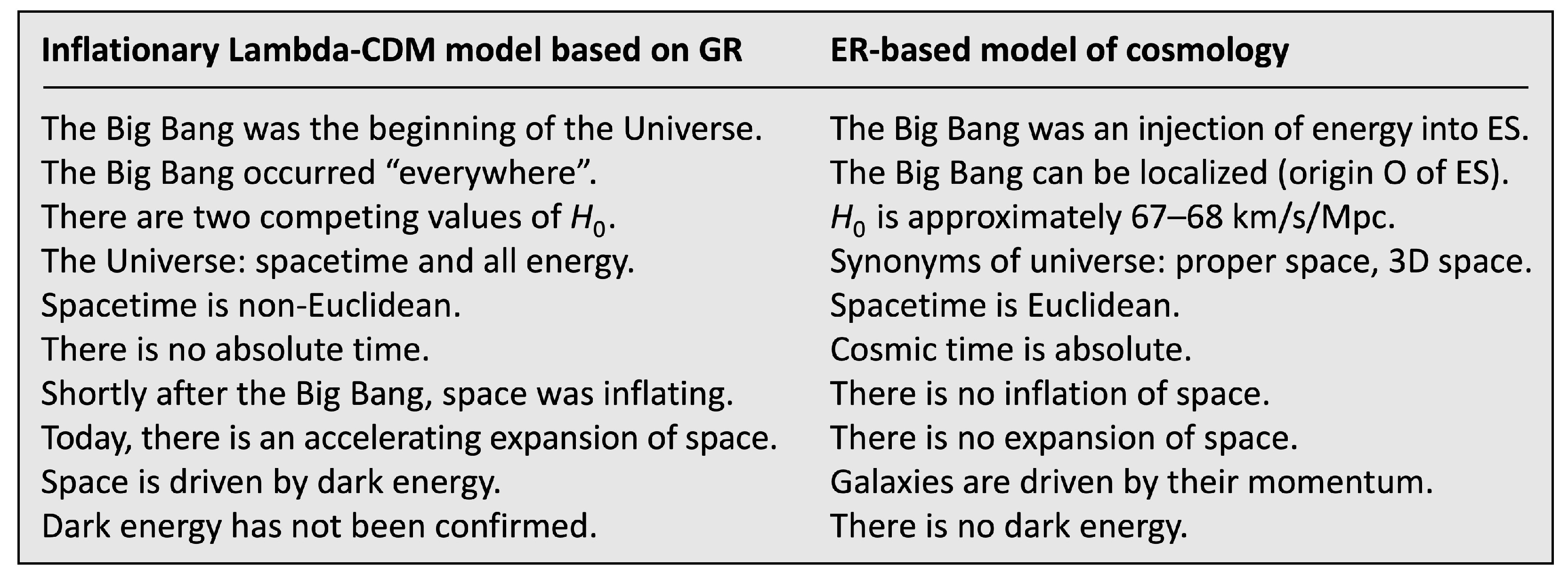
The Hubble tension and dark energy are solved by taking the 4D Euclidean geometry into account, and the 4D vector in particular. These results cast doubt on the Lambda-CDM model. GR works well as long as is not crucial, but it is crucial for high-redshift supernovae. Space is not driven by dark energy. Galaxies are driven by their momentum and maintain their recession speed with respect to Earth. Because of various effects (scattering, gravitational field, photon emission, pair production), some energy deviates from a radial motion in ES while maintaining the speed . Gravitational attraction enables near-by galaxies to move toward our galaxy. Table 1 compares two models of cosmology. Note that “the Universe” (Lambda-CDM model) and “universe” (ER-based model) are not the same thing. Each observer experiences three axes of ES as his universe. Cosmology benefits from ER. In Sect. 5.13 and 5.14, I show that QM also benefits from ER.
5.13. The Wave–Particle Duality
The wave–particle duality was first discussed by Niels Bohr and Werner Heisenberg [34]. It has bothered physicists ever since. In some experiments, objects behave like waves. In others, the same objects behave like particles (known as the “wave–particle duality”). One object cannot be both because a wave’s energy spreads out in space, whereas a particle’s energy is always localized in space. We overcome the duality by introducing another natural concept: All objects are “wavematters” (pure energy) that propagate through and oscillate in ES as a function of the parameter . In an observer’s view, wavematters reduce to wave packets if not tracked or else to particles if tracked.
In Fig. 8, observer R moves in the axis at the speed . Three wavematters , , and move in different 4D directions at the speed . For a better readability, a wavematter’s oscillation is drawn in the plane, although it can oscillate in any axis that is orthogonal to its propagation axis. does not move relative to R. Thus, it is automatically tracked and reduces to a particle (). In the 3D space of R, and reduce to wave packets () if not tracked or else to particles () if tracked. In the 3D space of R, moves at a speed less than . Thus, is what Louis de Broglie called a “matter wave” [35]. Erwin Schrödinger formulated his Schrödinger equation to describe matter waves [36]. In the 3D space of R, both and move at the speed . Thus, is the only wavematter that reduces for R to an electromagnetic wave packet or else to a photon. Light gives us a good idea of how wavematters move through ES.
Remarks: (1) “Wavematter” is not just a new word for the duality. It is a new concept, which tells us where the duality stems from and that it is experienced by observers only. Isn’t it enriching to learn that particles, matter waves, photons, and electromagnetic waves all stem from a common concept? (2) In today’s physics, there is no “photon’s view”. In ER, we can assign a 3D space and a proper time to each wavematter. In its view, its 4D motion disappears because of length contraction at the speed . In its 3D space, it is always at rest and reduces to a particle. (3) In a particle, a wavematter’s energy condenses to mass. Albert Einstein taught that energy and mass are equivalent [37]. Wavematters suggest that, likewise, a wave’s polarization and a particle’s spin are equivalent.
In double-slit experiments, light creates an interference pattern on a screen if it is not tracked through which slit single portions of energy are passing. The same applies if material objects, such as electrons, are sent through the double-slit [38]. Here light and matter behave like waves. In experiments on the photoelectric effect, an electron is released from a metal surface only if the energy of an incoming photon exceeds the binding energy of that electron. The photon must interact with that electron to release it. The interaction discloses their current position. They are tracked. Here light and matter behave like particles. Since an observer automatically tracks all objects that are slow in his 3D space, he classifies all slow objects—and thus all macroscopic objects—as matter. For a better readability, most of my ES diagrams do not show wavematters, but how they appear to observers.
5.14. Non-Locality
It was Erwin Schrödinger who coined the word “entanglement” in his comment [39] on the Einstein–Podolsky–Rosen paradox [40]. The three authors argued that QM would not provide a complete description of reality. Schrödinger’s neologism does not solve the paradox, but it demonstrates our difficulties in comprehending QM. John Bell [41] showed that QM is incompatible with local hidden-variable theories. Meanwhile, it has been confirmed in several experiments [42,43,44] that entanglement violates locality in an observer’s 3D space. Entanglement has been interpreted as a non-local effect ever since.
Up next, I show that ER is able to “untangle” entanglement. There is no violation of locality in ES, where all four axes are fully symmetric. In Fig. 9, observer R moves in the axis at the speed . There are two pairs of entangled wavematters. One pair was created at the point P and moves in opposite directions (equal to the axes of R) at the speed . The other pair was created at the point Q and moves in opposite directions at the speed . In the 3D space of R, the first pair (green) reduces to two entangled photons. The second pair (blue) reduces to two entangled material objects (for instance, electrons). R has no idea how two entangled objects are able to “communicate” in no time.
In the photons’ view (or electrons’ view), the axis (or else the axis) disappears because of length contraction at the speed . Thus, each pair stays together in its respective 3D space. Entangled objects have never been spatially separated in their view, but their proper time flows in opposite 4D directions. This is how two entangled objects are able to communicate in no time. Note that their opposite 4D vectors “flow of proper time” do not affect local communication as long as the twins stay together spatially. There is a “spooky action at a distance” (attributed to Einstein) in an observer’s view only.
The horizon problem and entanglement are solved exactly the same way: An observed region’s (or an observed object’s) 4D vector and its 3D space can differ from the observer’s 4D vector and his 3D space. All of this is possible, but only in ES, where all four axes are fully symmetric. The SO(4) symmetry of ES solves entanglement. It explains the entanglement of photons just as well as the entanglement of material objects, such as atoms or electrons [45]. Any measurement on one entangled twin will terminate its existence or tilt the axis of its 4D motion. In either case, the twins will not move in opposite 4D directions anymore. The entanglement is destroyed. In ER, non-locality is an obsolete concept.
5.15. The Baryon Asymmetry
In the Lambda-CDM model, almost all matter was created shortly after , when the temperature was high enough to enable pair production. But this process creates equal amounts of particles and antiparticles, and the process of annihilation annihilates equal amounts of particles and antiparticles. So, why do we observe more baryons than antibaryons (known as the “baryon asymmetry”)? In an observer’s view, wavematters reduce to wave packets or else to particles. Pair production creates particles and antiparticles, which annihilate each other very soon. Thus, there is one source of long-lived particles (reduction of wavematters), one source of short-lived particles (pair production), but only one source of short-lived antiparticles (pair production). This solves the baryon asymmetry.
ER also tells us why an antiparticle’s proper time seems “to flow backward”: Proper time flows in opposite 4D directions for any two wavematters created in pair production. The antiparticle’s 4D vector is reversed with respect to the particle’s 4D vector . In the antiparticle’s view, its proper time flows forward. ER predicts that any two wavematters created in pair production are entangled. This gives us a chance to falsify ER. Scientific theories must be falsifiable [46]. Note that galaxies moving in (not shown in Fig. 6 left) are not made up of antimatter. Only their flow of proper time is reversed with respect to galaxies moving in . Their physical charges are not reversed.
6. Conclusions
Modern physics lacks two qualities of time: absolute and vectorial. On the one hand, there is the cosmic evolution parameter (absolute time), which separates absolute past, present, and future. There is no absolute time in SR/GR. On the other hand, proper time is the length of a 4D Euclidean vector “flow of proper time” . There is no in SR/GR. While SR/GR work for all observers, the 15 mysteries solved in Sect. 5 show that the scope of SR/GR is limited. The 4D vector is crucial for objects that are very far away or entangled. Information hidden in and is not available in SR/GR. It is very unlikely that 15 solutions in different (!) areas of physics are 15 coincidences. Some of the 15 mysteries had been solved without ER, but with concepts that now prove obsolete. ER declares cosmic inflation, expanding space, dark energy, and non-locality obsolete. They are all subject to Occam’s razor. Occam shaves off obsolete concepts. No exceptions.
It was a wise decision to award Einstein the Nobel Prize for his theory of the photoelectric effect [47] and not for SR/GR. ER penetrates to a deeper level. Einstein, one of the most brilliant physicists ever, did not realize that the metric of nature is Euclidean. In fact, his instruction for synchronizing clocks blocks access to ER. He sacrificed absolute space and time. ER restores absolute time, but sacrifices the absolute nature of particles, matter waves, photons, and electromagnetic waves. In retrospect, two unfortunate practices of physicists delayed the formulation of ER: (1) Clocks measure , but is assigned a much smaller role in the equations of physics than . (2) Cosmologists are aware of , but when parameterizing worldlines in spacetime, the parameter is preferred over . For the first time ever, mankind now understands the nature of time: Cosmic time is the total distance covered in ES divided by . The human brain is able to imagine that we move at the speed . With that said, conflicts of mankind become all so small.
Is ER a physical or a metaphysical theory? This is a very good question because only in proper coordinates can we access ES, but the proper coordinates of other objects cannot be measured. I now explain why this is fine: We can always calculate these proper coordinates from ES diagrams as I showed in Eqs. (13a–c). Measuring is an observer’s source of knowledge, but ER tells us not to interpret too much into whatever we measure. Measurements are wedded to observers, whose concepts can be obsolete. I was often told that physics is all about observing. I disagree. We cannot observe quarks, can we? Regrettably, physicists have applied empirical concepts—which work well in our everyday life—to the very distant and the very small. This is why cosmology and QM benefit the most from ER. ER is a physical theory because it solves fundamental mysteries of physics.
Final remarks: (1) I only touched on gravity. We must not reject ER because gravity is still an issue. GR seems to solve gravity, but GR is incompatible with QM unless we add quantum gravity. Since ER solves mysteries of QM, quantum gravity is probably another obsolete concept. More studies are required to understand gravitational effects in ER. (2) Mysteries often disappear once the symmetry is matched. The symmetry group of natural spacetime is SO(4). (3) The parameter puts an end to all discussions about time travel. Does any other theory solve the mystery of time’s arrow as beautifully as ER? (4) Physics does not ask: Why is my reality a projection? Nor does it ask: Why is it a wave function? Projections are far less speculative than cosmic inflation plus expanding space plus dark energy plus non-locality. (5) It seems as if Plato had anticipated ER in his Allegory of the Cave [48]: Mankind experiences projections and cannot observe any reality beyond.
The key question in science is this: How does all of our insight into nature fit together without adding highly speculative concepts? It is this very question that leads to the truth. I laid the groundwork for ER and showed how powerful it is. Paradoxes are only virtual. The true pillars of physics are ER, SR/GR (for observers), and QM. Together they describe Mother Nature from the very distant down to the very small. Whenever we use empirical concepts, we must apply SR/GR. Whenever we use natural concepts, we must apply ER. Introducing a holistic view to physics is probably the most significant achievement of this paper. I demonstrated that SR/GR do not provide a holistic view. All observers’ views taken together do not make a holistic view because they still do not provide absolute time. Physics got stuck in its own concepts. Empirical concepts block our view of nature as a whole. Only in natural concepts does Mother Nature reveal her secrets. Everyone is welcome to solve even more mysteries by describing her in natural concepts.
Funding
No funds, grants, or other support was received.
Acknowledgements
I thank Siegfried W. Stein for his contributions to Sect. 5.11 and to Figs. 3, 5, 6. After several unsuccessful submissions, he decided to withdraw his co-authorship. I thank Matthias Bartelmann, Walter Dehnen, Cornelis Dullemond, Dirk Rischke, Jürgen Struckmeier, Christopher Tyler, Götz Uhrig, and Andreas Wipf for asking questions about the physics of ER. I am very grateful to all reviewers and editors for devoting their precious time to evaluating this new theory.
Comments
It takes open-minded editors and reviewers to evaluate a theory that heralds a paradigm shift. Taking SR/GR for granted paralyzes progress. I apologize for numerous preprint versions, but I received little support only. The preprints document my path. The final version is all that is needed. I did not surrender when top journals rejected my theory. Interestingly, I was never given any solid arguments that would disprove my theory. Rather, I was asked to try a different journal. Were the editors afraid of publishing a theory that is off the mainstream? Did they underestimate the benefits of ER? I was told that 15 solved mysteries are too much to be trustworthy. I disagree. Paradigm shifts often solve many mysteries at once. Even good friends refused to support me. Anyway, each setback motivated me to work out the benefits of ER even better. Finally, I succeeded in identifying an issue in SR/GR, which shows that Einstein’s general relativity is not as general as it seems.
Some physicists are not ready to accept ER because the SO(4) symmetry of ES seems to exclude waves. ER does not exclude waves. SO(4) is compatible with waves that propagate as a function of the parameter . A well-known preprint archive suspended my submission privileges. I was penalized because I identified an issue in Einstein’s SR and GR. The editor-in-chief of a top journal replied: “Publishing is for experts only.” One editor rejected my paper because it would “demand too much” from the reviewers. One editor could not imagine that the Hubble tension is solved without GR and called me a “pesky irritation”. I don’t blame anyone. Paradigm shifts are hard to accept. These comments shall encourage young scientists to stand up for good ideas even if it is hard work to oppose the mainstream. I was told that ER is “unscholarly research”, “fake science”, “too simple to be true”. Simplicity and truth are not mutually exclusive. Beauty is when they go hand in hand together.
Data availability
The data that support the findings of this study are available within the article.
Declarations
Conflict of Interest
The author has no conflicts to disclose.
References
- Einstein, A.: Zur Elektrodynamik bewegter Körper. Ann. Phys. 322, 891–921 (1905).
- Einstein, A.: Die Grundlage der allgemeinen Relativitätstheorie. Ann. Phys. 354, 769–822 (1905). [CrossRef]
- Minkowski, H.: Die Grundgleichungen für die elektromagnetischen Vorgänge in bewegten Körpern. Math. Ann. 68, 472–525 (1910).
- Rossi B., Hall, D.B.: Variation of the rate of decay of mesotrons with momentum. Phys. Rev. 59, 223–228 (1941). [CrossRef]
- Dyson, F.W., Eddington, A.S., Davidson, C.: A determination of the deflection of light by the sun’s gravitational field, from observations made at the total eclipse of May 29, 1919. Phil. Trans. R. Soc. A 220, 291–333 (1920).
- Ashby, N.: Relativity in the global positioning system. Living Rev. Relativ. 6, 1–42 (2003).
- Ryder, L.H.: Quantum Field Theory. Cambridge University Press, Cambridge (1985).
- Newburgh, R.G., Phipps Jr., T.E.: Physical Sciences Research Papers no. 401. United States Air Force (1969).
- Montanus, H.: Special relativity in an absolute Euclidean space-time. Phys. Essays 4, 350–356 (1991). [CrossRef]
- Montanus, H.: Proper Time as Fourth Coordinate. ISBN 978-90-829889-4-9 (2023). https://greenbluemath.nl/proper-time-as-fourth-coordinate/ (accessed 07 May 2025).
- Montanus, J.M.C.: Proper-time formulation of relativistic dynamics. Found. Phys. 31, 1357–1400 (2001). [CrossRef]
- Almeida, J.B.: An alternative to Minkowski space-time. arXiv:gr-qc/0104029 (2001).
- Gersten, A.: Euclidean special relativity. Found. Phys. 33, 1237–1251 (2003). [CrossRef]
- Newton, I.: Philosophiae Naturalis Principia Mathematica. Joseph Streater, London (1687).
- Hudgin, R.H.: Coordinate-free relativity. Synthese 24, 281–297 (1972). [CrossRef]
- Misner, C.W., Thorne, K.S., Wheeler, A.: Gravitation. W. H. Freeman and Company, San Francisco (1973).
- Wick, G.C.: Properties of Bethe-Salpeter wave functions. Phys. Rev. 96, 1124–1134 (1954). [CrossRef]
- Michelson, A.A., Morley, E.W.: On the relative motion of the Earth and the luminiferous ether. Am J. Sci. 34, 333–345 (1887).
- Church, A.E., Bartlett, G.M.: Elements of Descriptive Geometry. Part I. Orthographic Projections. American Book Company, New York (1911).
- Nowinski, J.L.: Applications of Functional Analysis in Engineering. Plenum Press, New York (1981).
- Abbott, B.P. et al.: Observation of gravitational waves from a binary black hole merger. Phys. Rev. Lett. 116, 061102 (2016). [CrossRef]
- Wald, R.M.: General Relativity. The University of Chicago Press, Chicago (1984).
- Hafele, J.C., Keating, R.E.: Around-the-world atomic clocks: predicted relativistic time gains. Science 177, 166–168 (1972). [CrossRef]
- Penzias, A.A., Wilson, R.W.: A measurement of excess antenna temperature at 4080 Mc/s. Astrophys. J. 142, 419–421 (1965). [CrossRef]
- Hubble, E.: A relation between distance and radial velocity among extra-galactic nebulae. Proc. Natl. Acad. Sci. U.S.A. 15, 168–173 (1965).
- Lemaître, G.: Un univers homogène de masse constante et de rayon croissant, rendant compte de la vitesse radiale des nébuleuses extra-galactiques. Ann. Soc. Sci. Bruxelles A 47, 49–59 (1927).
- Linde, A.: Inflation and Quantum Cosmology. Academic Press, Boston (1990).
- Guth, A.H.: The Inflationary Universe. Perseus Books, New York (1997).
- Aghanim, N. et al.: Planck 2018 results. VI. Cosmological parameters. Astron. Astrophys. 641, A6 (2020).
- Riess, A.G. et al.: A comprehensive measurement of the local value of the Hubble constant with 1 km s−1 Mpc−1 uncertainty from the Hubble Space Telescope and the SH0ES team. Astrophys. J. Lett. 934, L7 (2022). [CrossRef]
- Perlmutter, S. et al.: Measurements of Ω and Λ from 42 high-redshift supernovae. Astrophys. J. 517, 565–586 (1999).
- Riess, A.G. et al.: Observational evidence from supernovae for an accelerating universe and a cosmological constant. Astron. J. 116, 1009–1038 (1998).
- Turner, M.S.: Dark matter and dark energy in the universe. arXiv:astro-ph/9811454 (1998).
- Heisenberg, W.: Die physikalischen Prinzipien der Quantentheorie. Hirzel, Leipzig (1930).
- de Broglie, L.: The reinterpretation of wave mechanics. Found. Phys. 1, 5–15 (1970).
- Schrödinger, E.: An undulatory theory of the mechanics of atoms and molecules. Phys. Rev. 28, 1049–1070 (1926). [CrossRef]
- Einstein, A.: Ist die Trägheit eines Körpers von seinem Energieinhalt abhängig? Ann. Phys. 323, 639–641 (1905).
- Jönsson, C.: Elektroneninterferenzen an mehreren künstlich hergestellten Feinspalten. Z. Phys. 161, 454–474 (1961).
- Schrödinger, E.: Die gegenwärtige Situation in der Quantenmechanik. Naturwissenschaften 23, 807–812 (1935). [CrossRef]
- Einstein, A., Podolsky, B., Rosen, N.: Can quantum-mechanical description of physical reality be considered complete? Phys. Rev. 47, 777–780 (1935). [CrossRef]
- Bell, J.S.: On the Einstein Podolsky Rosen paradox. Physics 1, 195–200 (1964).
- Freedman, S.J., Clauser, J.F.: Experimental test of local hidden-variable theories. Phys. Rev. Lett. 28, 938–941 (1972). [CrossRef]
- Aspect, A., Dalibard, J., Roger, G.: Experimental test of Bell’s inequalities using time-varying analyzers. Phys. Rev. Lett. 49, 1804–1807 (1982).
- Bouwmeester, D. et al.: Experimental quantum teleportation. Nature 390, 575–579 (1997).
- Hensen, B. et al.: Loophole-free Bell inequality violation using electron spins separated by 1.3 kilometres. Nature 526, 682–686 (2015). [CrossRef]
- Popper, K.: Logik der Forschung. Julius Springer, Vienna (1935).
- Einstein, A.: Über einen die Erzeugung und Verwandlung des Lichtes betreffenden heuristischen Gesichtspunkt. Ann. Phys. 322, 132–148 (1905). [CrossRef]
- Plato: Politeia, 514a.
Fig. 1.
Orthogonal projections and two approaches to describing nature. Left: How to project ES to an object’s reality. Right: ER and SR/GR describe nature in different concepts.
Fig. 1.
Orthogonal projections and two approaches to describing nature. Left: How to project ES to an object’s reality. Right: ER and SR/GR describe nature in different concepts.
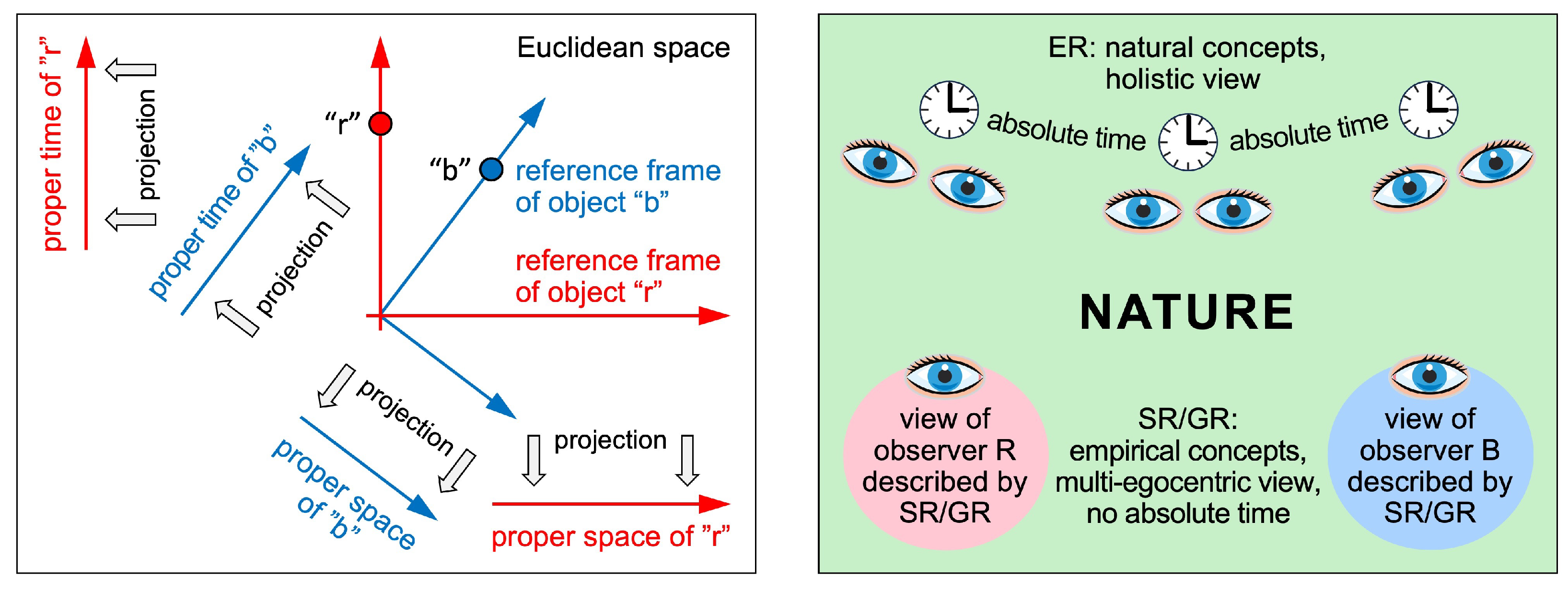
Fig. 2.
Minkowski diagram and ES diagram of two clocks “r” and “b”. Left: “b” is slow with respect to “r” in . Coordinate time is relative (“b” is at different positions in and ). Right: “b” is slow with respect to “r” in . Cosmic time is absolute (“r” is in at the same position as “b” in ).
Fig. 2.
Minkowski diagram and ES diagram of two clocks “r” and “b”. Left: “b” is slow with respect to “r” in . Coordinate time is relative (“b” is at different positions in and ). Right: “b” is slow with respect to “r” in . Cosmic time is absolute (“r” is in at the same position as “b” in ).
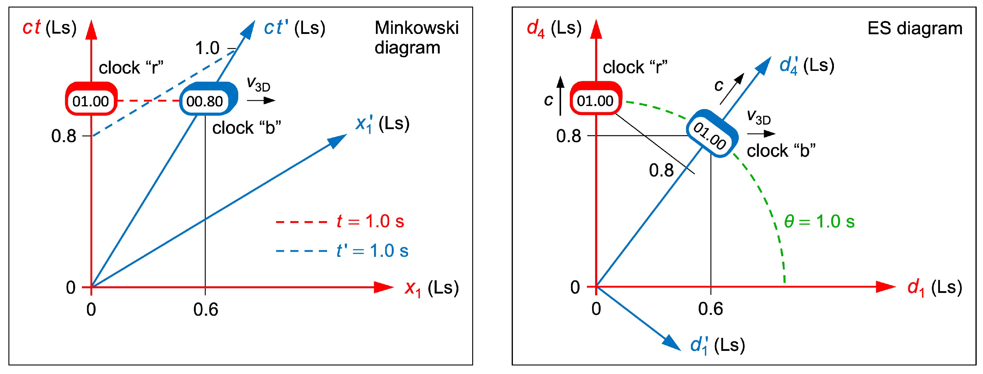
Fig. 3.
ES diagrams of two rockets “r” and “b”. Observer R (or B) is in the rear end of “r” (or else “b”). Left: “r” moves in the axis. “b” moves in the axis. In the 3D space of R, “b” contracts to . Right: The ES diagram has been rotated only. In the 3D space of B, “r” contracts to
Fig. 3.
ES diagrams of two rockets “r” and “b”. Observer R (or B) is in the rear end of “r” (or else “b”). Left: “r” moves in the axis. “b” moves in the axis. In the 3D space of R, “b” contracts to . Right: The ES diagram has been rotated only. In the 3D space of B, “r” contracts to
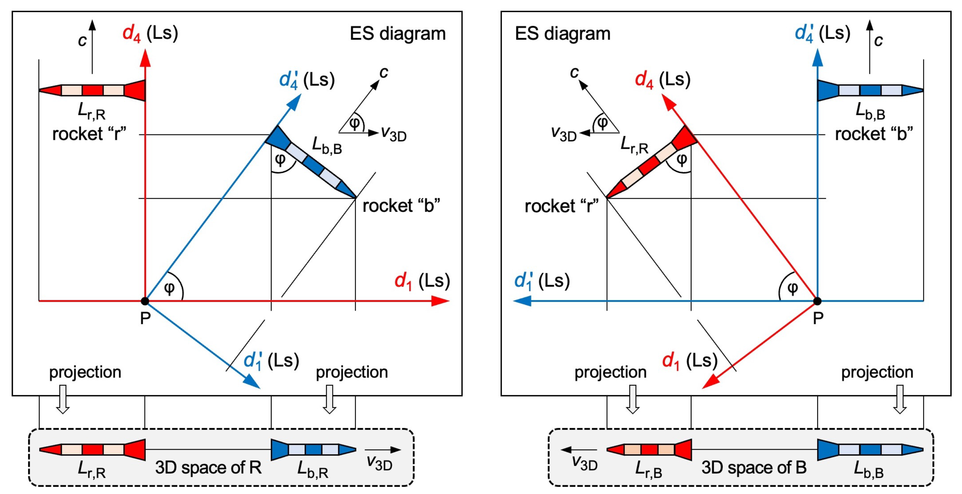
Fig. 4.
ES diagram of two clocks “r” and “b” and Earth. Clock “b” accelerates toward Earth. The axis is drawn curved because it indicates the current 4D motion of “b”.
Fig. 4.
ES diagram of two clocks “r” and “b” and Earth. Clock “b” accelerates toward Earth. The axis is drawn curved because it indicates the current 4D motion of “b”.
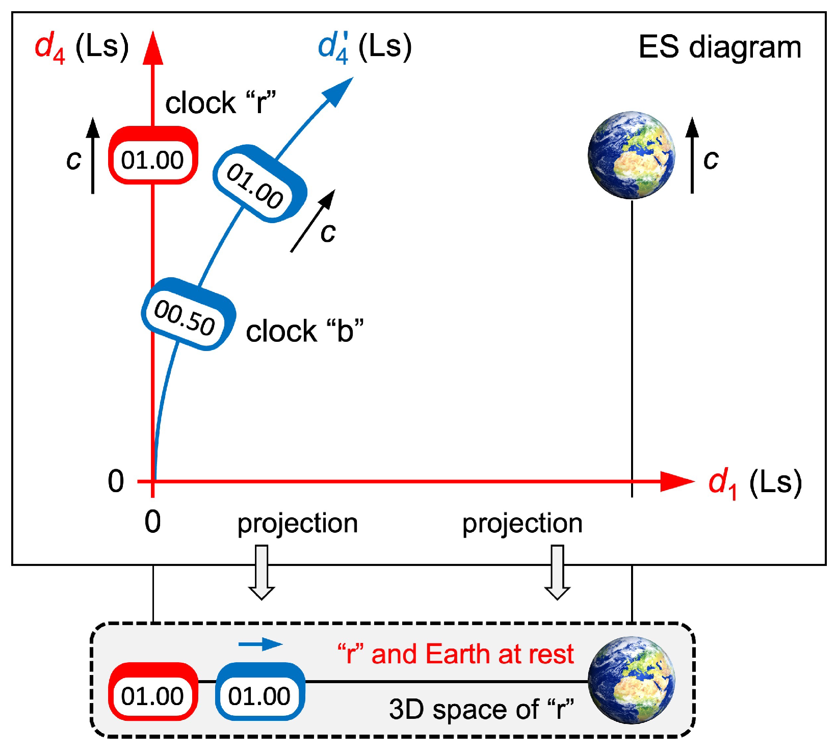
Fig. 5.
Three instructive problems. Left: Two objects move through ES. The orange circle shows where a signal emitted by “b” at is at . In ES, the objects do not collide. In the 3D space of “r”, they do. Center: In ES, the wire escapes from the rocket. In the 3D space of the wire, it does not. Right: In ES, the sun escapes from Earth’s orbit. In the 3D space of the sun, it does not.
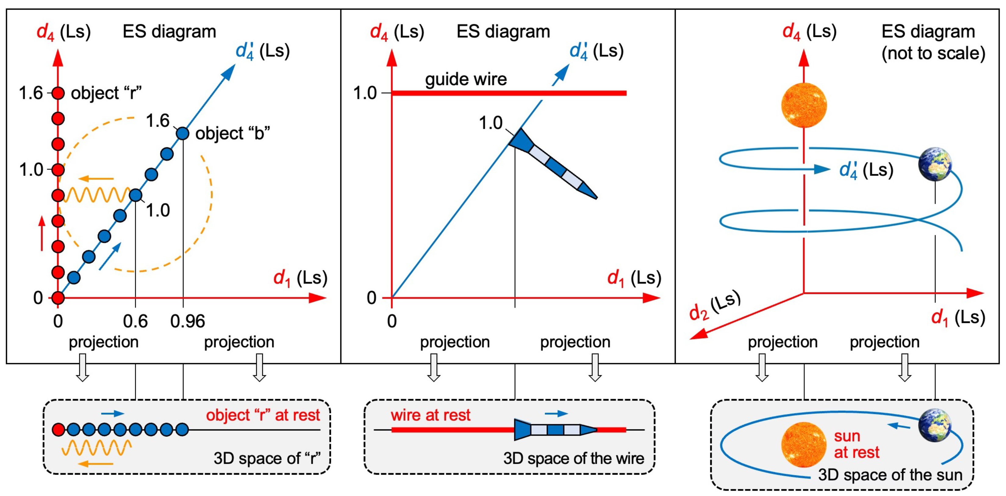
Fig. 6.
ER-based model of cosmology. The green arcs show parts of a 3D hypersurface. The orange circles show where most of the energy emitted by G or S at the time is today. Left: G recedes from O at the speed and from the axis at the speed . Right: If a star happens to be at the same distance today at which the supernova of S occurred, recedes more slowly from than S.
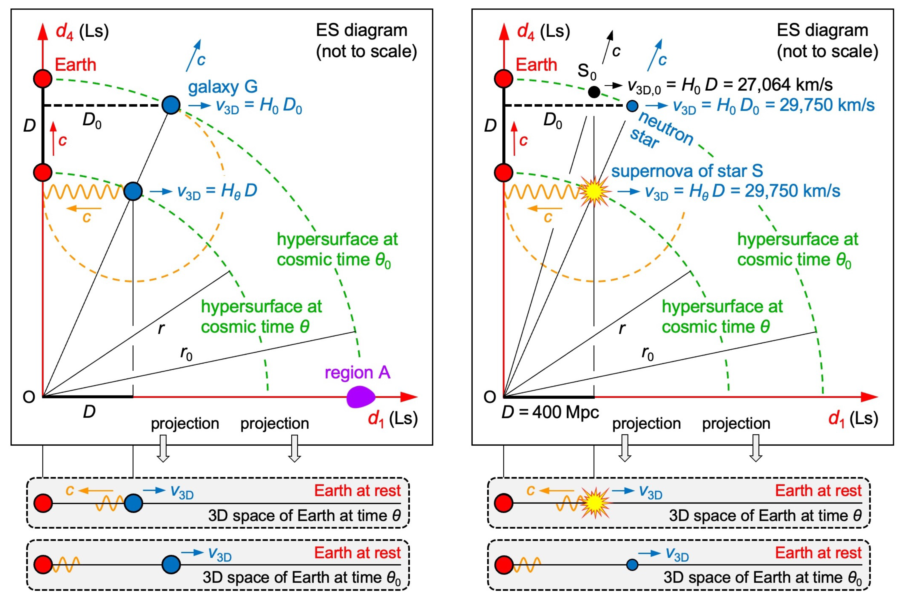
Fig. 7.
Hubble diagram of simulated supernovae. The horizontal axis is for the red points or else for the blue points. The red points, calculated from Eq. (20), do not yield a straight line because is not a constant. The blue points, calculated from Eq. (21), yield a straight line.
Fig. 7.
Hubble diagram of simulated supernovae. The horizontal axis is for the red points or else for the blue points. The red points, calculated from Eq. (20), do not yield a straight line because is not a constant. The blue points, calculated from Eq. (21), yield a straight line.
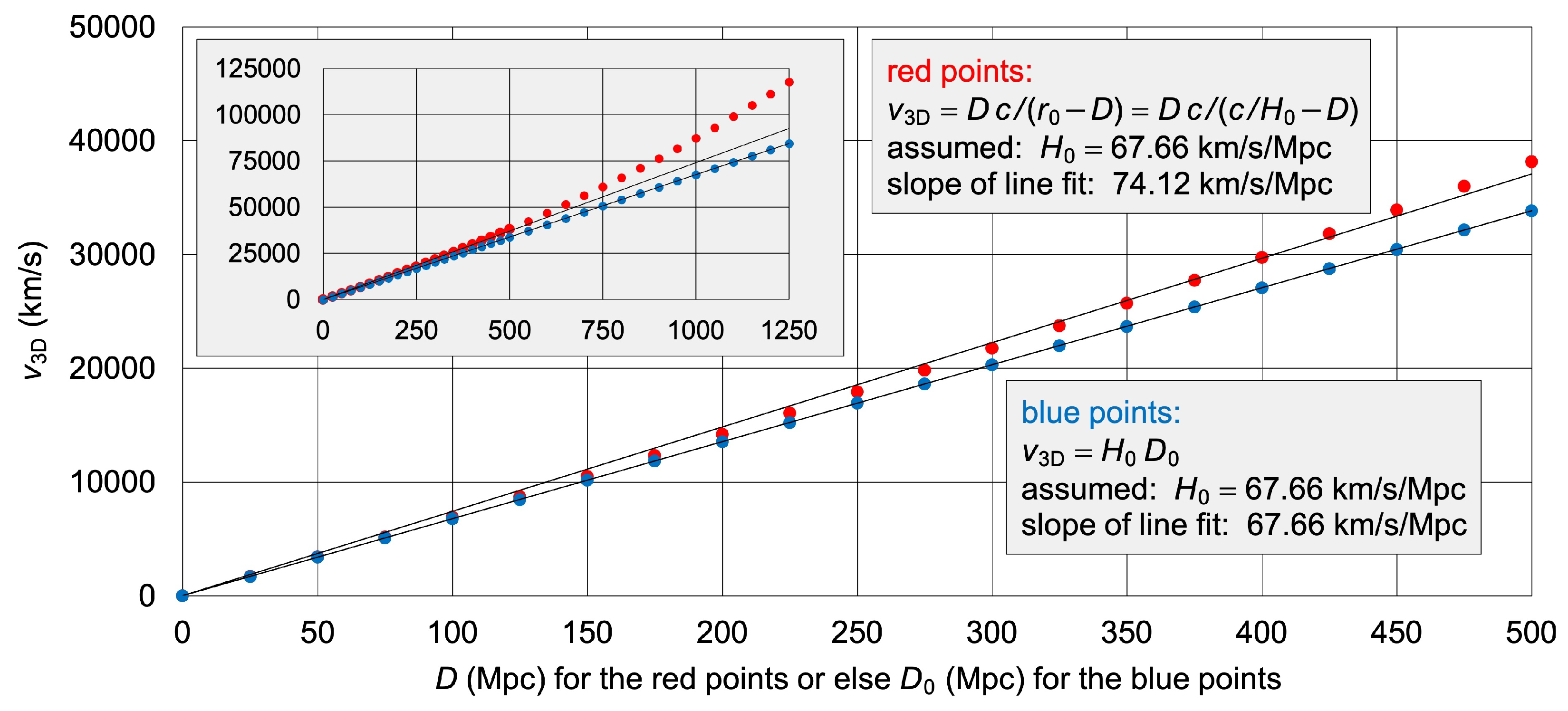
Fig. 8.
Wavematters. Observer R moves in the axis. In his 3D space, and reduce to wave packets () if not tracked or else to particles () if tracked. : possibly an atom of R. : matter wave. : moving particle. : electromagnetic wave packet. : photon.
Fig. 8.
Wavematters. Observer R moves in the axis. In his 3D space, and reduce to wave packets () if not tracked or else to particles () if tracked. : possibly an atom of R. : matter wave. : moving particle. : electromagnetic wave packet. : photon.
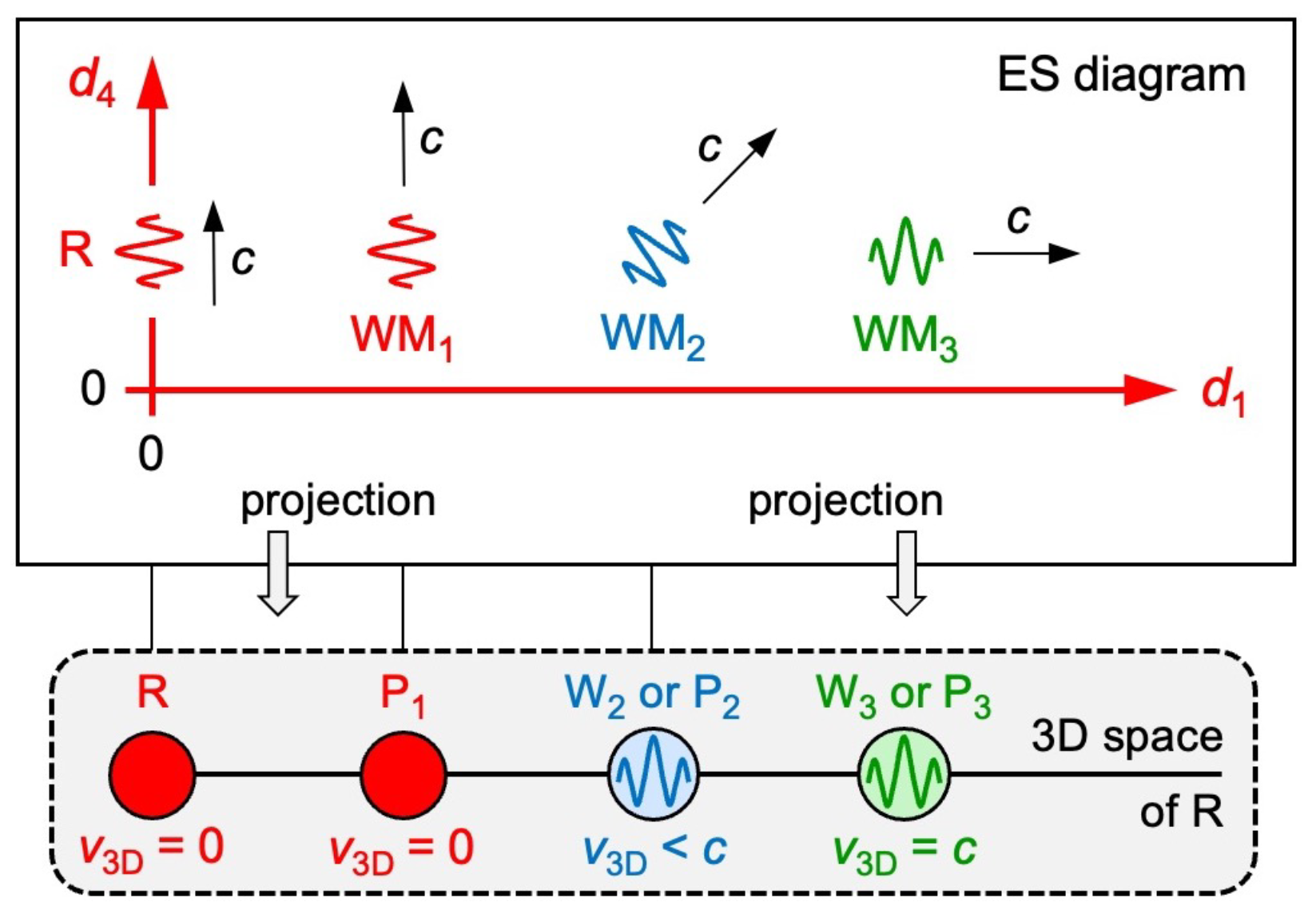
Fig. 9.
Entanglement. Observer R moves in the axis at the speed . Two entangled wavematters (green) reduce to photons. Two entangled wavematters (blue) reduce to electrons. In the photons’ 3D space (or electrons’ 3D space, not shown), the photons (or else electrons) stay together.
Fig. 9.
Entanglement. Observer R moves in the axis at the speed . Two entangled wavematters (green) reduce to photons. Two entangled wavematters (blue) reduce to electrons. In the photons’ 3D space (or electrons’ 3D space, not shown), the photons (or else electrons) stay together.
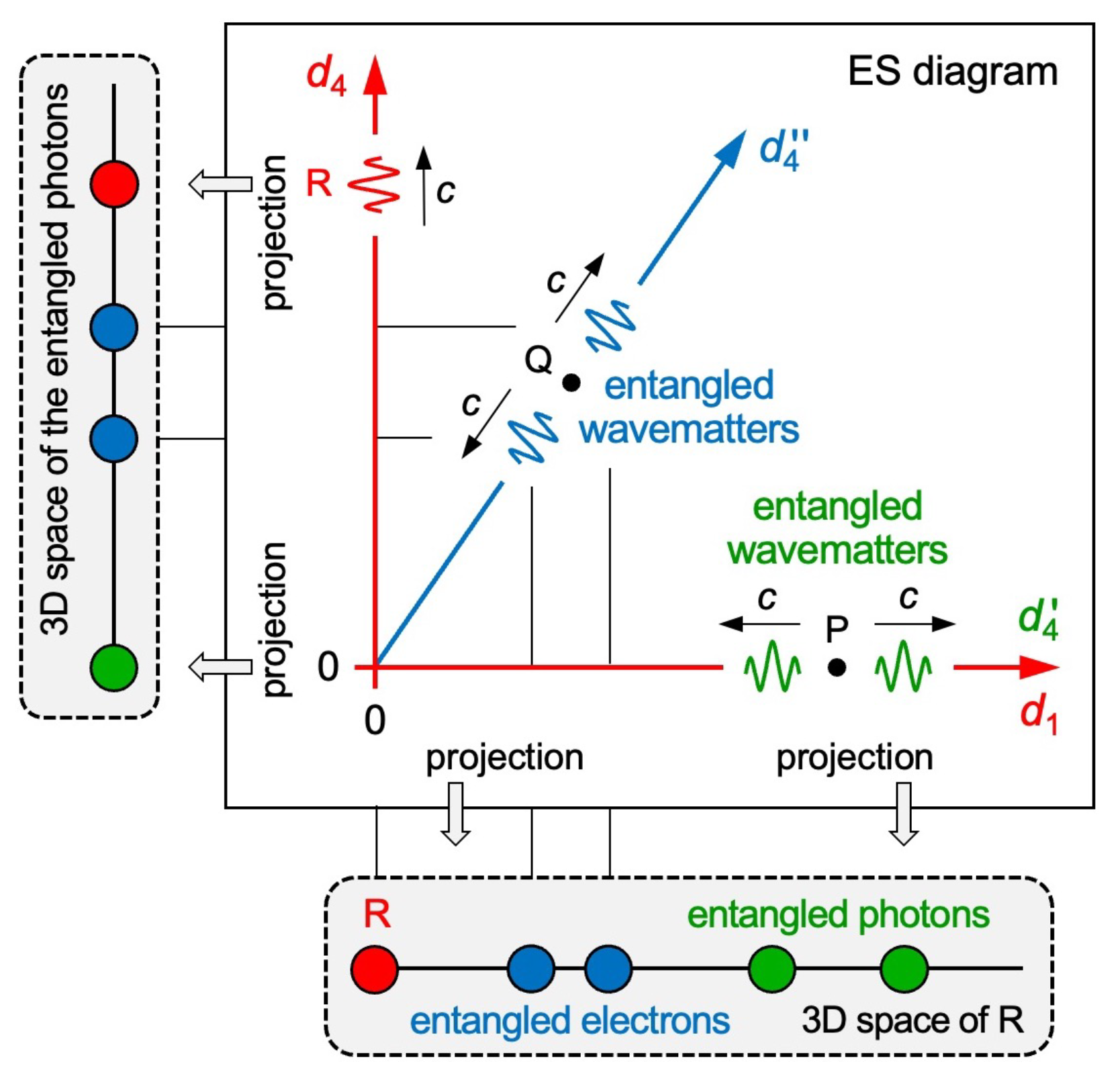
Table 1.
Comparing two models of cosmology.
Disclaimer/Publisher’s Note: The statements, opinions and data contained in all publications are solely those of the individual author(s) and contributor(s) and not of MDPI and/or the editor(s). MDPI and/or the editor(s) disclaim responsibility for any injury to people or property resulting from any ideas, methods, instructions or products referred to in the content. |
© 2025 by the authors. Licensee MDPI, Basel, Switzerland. This article is an open access article distributed under the terms and conditions of the Creative Commons Attribution (CC BY) license (http://creativecommons.org/licenses/by/4.0/).
Copyright: This open access article is published under a Creative Commons CC BY 4.0 license, which permit the free download, distribution, and reuse, provided that the author and preprint are cited in any reuse.


