

Submitted:
12 February 2023
Posted:
13 February 2023
Read the latest preprint version here
Abstract
The FRW model of cosmology assumes a Universe with uniform pressure and density everywhere in space at a given time. But at the largest scales, the Universe has a web-like structure surrounding large voids, violating these assumptions. Furthermore, a given region of spacetime is describable only by a single metric and therefore it cannot be that the Universe is modelled as an FRW perfect fluid since this would be the incorrect description of both the web and the voids. The cosmic web must be described by metrics with non-zero energy-momentum tensors with non-uniform pressure and density describing the matter within it. Therefore, the model of cosmology describing the expansion of the Universe must be a vacuum solution describing the empty spaces in the Universe surrounded by an infinite, massive shell (the surrounding Universe). The internal Schwarzschild metric is that model. The source of the Schwarzschild metric is shown to be at the event horizon, a location/time of infinite density, not at the singularity, as it is currently assumed. The spatial homogeneity of the metric is demonstrated by visualizing the geometry in the extrinsic "Kruskal-Szekeres" coordinates (visualized in 1+2 dimensions). Using the coordinate age of the Universe and transition redshift, this predicts the accelerated expansion, the Hubble diagram fits currently available cosmological data, and it gives a Hubble constant H0 of 71.6km/s/Mpc. The angular term of the metric describes the relativistic kinematic precession effect known as Thomas Precession which can be interpreted as spin about the time dimension.
Keywords:
Cosmology
; Black holes
; Dark Energy
; Schwarzschild metric
1. Motivation and Roadmap
The current model of cosmology is based on the FRW metric, which comes from the assumption that the Universe is accurately modelled as perfect fluid. This means that we are modelling the Universe as having uniform density and pressure at all points in space. While this may be a good approximation for the early pre-recombination Universe, the perfect fluid assumption is clearly no longer a valid one in the later Universe. We observe that the Universe is not a uniform distribution of galaxies, but rather a web-like structure of matter surrounding large voids. Thus, the pressure and density is surely not uniform at all locations in space, making the perfect fluid assumption less and less accurate as the Universe expands and cools.
Furthermore, it is notable that a given region of spacetime can only be described by one metric. This means that the region containing a star, for example, is not described by the FRW metric, it is described by a spherically-symmetric metric with a radially-dependant mass density and pressure where the metric must match the external Schwarzschild metric at the star’s outer radius. Therefore, the cosmic filaments cannot be described by the FRW metric because they are not perfect fluids (with regions of uniformly dense gas being the exception) and the spacetime in those regions will be described by metrics whose mass distribution matches the configurations of the filaments. What this implies is that a cosmological metric (one that accurately describes the expansion of the Universe) must be a vacuum solution describing the empty spaces surrounded by the matter in the Universe. This empty space differs from Minkowski space in that the empty spaces in the Universe are surrounded by the infinite mass of the Universe and therefore should be modelled as a spherically-symmetric vacuum surrounded by a shell of infinite mass.
It will be argued in this paper that the metric properly describing the vacuum of the Universe, including its accelerated expansion, is the internal Schwarzschild metric. Section 2 demonstrates how the source of both the external and internal metrics are not at , but rather at the event horizon which represents an infinitely dense shell as viewed from the outside in the case of the external metric, and an infinitely dense shell as viewed from the inside in the case of the internal metric. Justification for the internal metric representing a vacuum surrounded by a shell at infinity comes from looking at the geometry in Kruskal coordinates and noting that the horizon is located at spatial infinity for the internal metric. This means in the internal metric, the shell has an infinite Schwarzschild radius and therefore infinite mass. In both metrics, as will be shown, these shells look like infinitely dense points in the frame of an observer approaching the shell in space for the case of the external metric and in time for the case of the external metric. The temporal nature of the spatial expansion and contraction of the internal metric matches what we observe in regards to the structure of the Universe. Furthermore, in Section 3, we demonstrate that it would be impossible to fall past the horizon from the outside due to length contraction effects for observers approaching the horizon.
In Section 2, we also demonstrate that surfaces of constant time in the internal metric can be visualized as a collection of 2-sheeted hyperboloids analogous to how the external metric at a given radius can be visualized as a collection of one sheet hyperboloids. The 2-sheeted hyperbolic nature of the metric changes the interpretation of the angular term relative to the external metric, and it is shown that the metric describes a Universe that is isotropic, homogeneous in space and inhomogeneous in time, as our Universe has been observed to be. It is also demonstrated that the angular term of the internal metric comes from the kinematic relativistic effect known as Thomas Precession. This precession acts as an intrinsic ’spin’ around the time dimension. In Section 7, it is shown how this term gives rise to Coriolis accelerations that affect curvilinear motion of massive objects as well as gravitational lensing angles.
In Section 6 we solve for the unknowns for the internal Schwarzschild metric, namely our current cosmological position in the metric and the counterpart of the Schwarzschild radius, using existing cosmological data. The model is then used to calculate relevant cosmological parameters and it is found that the model fits the cosmological data very well.
In Section 10, the internal metric is interpreted as having an imaginary (as in complex numbers) radius which gives us the 2-sheeted hyperbolic structure. This 2-sheeted geometry gives us a Universe and Anti-Universe falling in opposite directions of time relative to each other. The Universe and anti-Universe are falling through the imaginary time dimension described in that section. It is shown that the Universe and Anti-Universe undergo an expansion phase followed by a collapse, where they annihilate with each other and pair production then gives birth to a new pair of Universes as the cycle repeats.
In Section 12, we place the external metric in the background cosmology of the internal metric and show that a Black Hole event horizon can never form during the expansion phase. We see that gravity becomes repulsive during the collapse phase and would-be Black Holes become White Holes. This is a consequence of the Universe moving in the opposite direction of time during collapse relative to expansion.
We will begin the argument by examining the geometry of the full Schwarzschild metric in detail.
2. The Schwarzschild Geometry
The Schwarzschild metric is the simplest non-trivial solution to Einstein’s field equations. It is the metric that describes every spherically symmetric vacuum spacetime. The the external and internal forms of metric can be expressed as (coordinates in the external metric are primed to distinguish them from the internal metric coordinates):
Equation (1) is the external metric with being the timelike coordinate and being the spacelike coordinate. The Schwarzschild radius of the metric is given by in units with . We use the prime notation for the coordinates here to distinguish the external coordinates from the internal coordinates. The external metric is the metric for an eternally spherically-symmetric vacuum centered in space. This metric is also used to describe the vacuum outside a spherically symmetric object occupying a finite amount of space with a finite mass (like a star or planet). This metric as written in Equation (1) becomes the Minkowski metric as .
Equation (2) is the internal metric with t being the spacelike coordinate and r being the timelike coordinate. This metric is currently believed to describe the interior of a Black Hole. But consider the case of a spherically-symmetric vacuum surrounded by a spherically-symmetrically distributed infinite amount of mass. This would be a spacetime surrounded by a shell with an infinite Schwarzschild radius (because the mass of the shell is infinite). Since this is a spherically symmetric vacuum, it must be described by the Schwarzschild metric. This is also the description of spherically-symmetric vacua in our Universe, since the surrounding Universe is effectively a shell of infinite mass (every region of the Universe is light-like connected to the Big Bang in all directions, which acts as a shell of infinite mass/Schwarzschild radius). Therefore, the internal metric describes the spacetime of the pockets of empty space in the Universe. The constant u in the internal metric is a time constant whose value in years will be later derived from cosmological data. Choosing a value for this constant amounts to choosing the units of time for analysis. This metric is essentially the Minkowski metric with a variable speed of light, which can also be interpreted as an expanding or collapsing space.
So the Schwarschild metric describes the curved spacetime caused by an infinitely dense shell from two perspectives:
- The external metric describes the spacetime around an infinitely dense shell of finite mass and radius in the frame of an observer infinitely far away from the shell
- The internal metric describes the spacetime inside an infinitely dense shell located at infinity in the frame of an observer at rest inside the shell. In the case of the Universe, the shell would be the entire Universe at time (as will be shown, the scale factor is zero there and therefore we have infinite coordinate density).
Figure 1 shows the Kruskal-Szekeres coordinate chart1 for both the internal and external metrics where light travels on 45 degree lines on the chart. This will help illustrate the above points more clearly.
On this diagram, the lines represent the infinitely dense shells in both scenarios. We can see that at (the ’Horizon”), both metrics are the same. The origin location/time describes an infinitely dense point in space for the external solution (this is shown formally in Section 3) for all time and a time at which all infinite space is contracted for the external solution. The lines are light-like because light cannot escape an infinitely dense region of space, regardless of the mass (i.e., the external observer cannot receive light emitted from the Schwarzschild radius and the internal observer cannot receive light from the time when space was infinitely contracted). The different quadrants of Figure 1 will be examined in Section 9. We can also see in Figure 1 that for the internal metric, the horizon is located at , meaning the Schwarzschild radius and therefore mass of the shell is infinite (because t is the spacelike coordinate). Thus, it is clear from the geometry that the source masses of the Schwarzschild metric are not concentrated at (which is currently assumed and accepted by most physicists today, but is not anywhere mathematically implied or demanded in the derivation of the Schwarzschild metric), but rather at the event horizon itself.
Another way to look at the internal metric is that it describes an infinitely dense source that exists at a location in time, not space. The vacuum surrounding the source is a vacuum in time (i.e., the r dimension is a vacuum). Just like the density of a massive free falling shell in a spatial vacuum is governed by the external metric, the density of a spherically symmetric, infinite 3D volume of space that physically moves through time (i.e., in a presentist Universe where only the present contains matter and energy and the past and future are vacuums) is governed by the internal metric. The source in this case would be the so-called ’Big Bang’, which, from our present perspective looks like an infinitely dense shell a finite time in the past away from us in all directions. It will be shown that the scale factor of the metric is zero at that time meaning that the infinite 3D space is compressed there, which means the mass of the source for the internal metric must be infinite, which is exactly what we expect for the Universe at a time when the scale factor is zero. As will be shown in Section 3, the horizon of the external metric looks like a shell (viewed from the outside) from far away, but becomes an infinitely dense point in the frame of an observer approaching it. Likewise, the Big Bang looks like an infinitely dense shell (viewed from the inside) at times later than the Big Bang, but looks like an infinitely dense point (because the proper distance goes to zero regardless of coordinate distance at that time) in the frame of an observer in the Universe as the Universe approaches that time. In other words, both the internal and external metrics look the same in the frame of an observer approaching the source, which is to be expected since they have the same mathematical description there.
Now we must show that the space in the internal metric is isotropic and homogeneous. The equation for a 2D hyperboloid surface embedded in three dimensions is given by:
For our purposes, we will be considering the special case where , which gives the one and two sheeted hyperboloids of revolution. Next, we note the following relationship with regards to the Kruskal coordinates:
Equation (4) is only for one dimension of space, but we know that the metric is spherically symmetric and can therefore extend Equation (4) to 2 spatial dimensions by simply adding a Y coordinate to get an equation that matches the form of Equation (3) where :
Equation (5) describes 2D hyperboloid surfaces for a given r where the external metric has positive and the internal metric has negative . This means that the external metric describes a 1-sheet hyberboloid while the internal metric describes a 2-sheeted hyperboloid.
We will for now focus on regions I and II from Figure 1, where region I captures the external metric and region II captures the internal metric. If we choose some constant value of in each region and plot Equation (5) for each region, we get the surfaces shown in Figure 2.
In the internal case where we have two separate sheets, we will only focus on the top sheet for now. The meaning of the bottom sheet will be discussed in Section 9. In the external metric, the sheet represents an equatorial circle of space around the central body at all times. This circle is on a plane with a normal at the center and pointed vertically in Figure 2. If we then consider circles on all planes whose normals are at different angles relative to the normal of the plane we are currently visualizing, we get a 2D spherical surface representing the space surrounding the central body at constant r.
Light cones in Figure 2 are oriented vertically and light travels on 45 degree lines. If we consider the right side of Figure 2, representing the external metric, choose any point on the surface and project a past and future light cone out of that point (this will just be a vertical cone centered at that point). We see that the external metric is anisotropic and inhomogeneous because the surface is asymmetric relative to the surface left and right as well as into and out of the page. But the light cone is symmetric vertically relative to the surface. We can see this because we are allowed to circularly and/or hyperbolically rotate any point to a point at the throat of the surface and the space will remain unchanged. This is because the metric is spherically symmetric (representing circular rotations) and static (representing hyperbolic rotations). It becomes clear that the cone is vertically symmetric relative to the surface at the throat since both the cone and surface are vertically symmetric in a plane parallel to the throat. So any point we choose to start with can be moved to the throat of the surface and we see that the cone is vertically symmetric relative to the surface when we move a point there.
Now consider the top sheet on the left side of Figure 2 representing the internal metric. Again choose any point on the surface and project a past and future light cone vertically from that point. Just like in the case of the external metric, we can move that point anywhere on the surface to the apex of the surface by hyperbolically and/or circularly rotating the point there (and the space will remain unchanged). When the point is rotated to the apex, we see then that the light cone is symmetric relative to the surface left and right and into and out of the page. This symmetry means the internal metric is isotropic and homogeneous. The cone is not vertically symmetric relative to the surface, however, and that reflects the fact that the internal metric is not static.
The above arguments tell us something important about the Schwarzschild metric. When the metric is derived from Einstein’s field equations, it is usually done from the perspective of the external metric. In the derivation, we assume spherical symmetry and a static spacetime. It is notable that in spite of the static assumption, we still get an internal metric that is non-static. This is because the static assumption for the external metric is actually an implicit assumption of hyperbolic symmetry. Therefore, we can more correctly state that the Schwarzschild metric is the vacuum solution to Einstein’s field equations that is both spherically and hyperbolically symmetric. This hyperbolic symmetry manifests itself as a static metric when the time coordinate is hyperbolic (the external metric) and an isotropic and homogeneous metric when the space coordinate is hyperbolic (the internal metric)
Let us examine the Killing vectors for the geometry on a surface of constant r in the internal metric. The circles on the sheets on the left side of Figure 2 are circles of constant t. Figure 3 shows these contours on a plane with the Killing/Basis vectors and plotted on the contours (and we set in this case). This represents a 2D slice of space at a fixed time r.
First, we see that the t coordinate is a spatial radius because the vectors all point out from the center (which is an arbitrary point in space) in all directions and they have the same length everywhere at a given time r. But we also see that the vector has the same magnitude at all t since, because we have , the length of the vector will be time r which is constant over space in this example. The length of the vector is not even zero at since, again, r is constant even at that point. Also, as will be discussed in Section 7, a rotation of is a rotation of the entire surface about a point which is why the vectors are depicted as rotations in the plane. This is because the radius in the angular term of the metric is a time r, not the spatial radius t. Thus, rotations in this metric are describing a kind of ’spin’ around a time axis (where the time dimension runs perpendicular to the page at all points) as opposed to a revolution in space. So you can have a non-zero rotation in the metric without moving through space (remaining at ), implying that the angular term of the metric is describing a spin, which is discussed in Section 7. Curvilinear motion through space is also discussed in Section 8.
Since we are looking at a 2D example in Figure 3 and we have 2 spacelike Killing vectors of constant length everywhere for a given time r, we see that the surface is therefore homogeneous and isotropic. This is easily extended to 3D by imagining that the concentric circles in Figure 3 are concentric spheres, and given the spherical symmetry of the metric, the symmetries described in the 2D case will therefore apply to the full 3D case.
Now imagine we are situated at some point in empty space in the Universe facing in some direction. There is a plane of infinite space at the present time perpendicular to the direction we are facing. This plane is the hyperbolic sheet depicted on the left side of Figure 2 where we are situated at the apex of the sheet. So the direction we are facing is the normal vector to this sheet (with the vector origin at the apex of the sheet) and just like in the external case, there are similar planes constructed from normals at all different angles to the direction we chose to face and when we put all of these together, we get an infinite 3D space at the present time.
But the points on this collection of sheets at are spacelike to us because they all exist at the same time as us and we can only see points on past sheets whose light has had time to reach us. Light paths in Figure 1 are lines at 45 degrees and light cones in Figure 2 are oriented vertically where the beginning of the Universe is at the origin between the two sheets and time moves forward as the top sheet moves up the diagram vertically. So we can construct an image of what a 2D slice of the Universe would look like to us in this geometry with our position at the center. Figure 4 shows the present sheet () where we are positioned in space at the apex of the sheet. We then show a cross section of that sheet on the Kruskal-Szekeres coordinate chart with the past light cone shown (dashed lines at 45 degrees emanating from at ). That light cone intersects past sheets of constant (past sheets not shown in the top left of Figure 4 but are represented by the hyperbolas the dashed lines intersect in the top right of the figure) and these intersections are projected onto the plane at the origin to give us a 2D image of our past light cone of the Universe. The density of the coordinates at different radii (and therefore times) is depicted with the shading inside the projection.
Despite the hyperboloic nature of the spacelike planes, space still looks flat from our perspective because our past light cone intersects past surfaces as circular cross-sections. As we can see in the lower projection in Figure 4, concentric circles around the center of the projection (marked with ’x’) are circles of constant distance and time from us. So we see that as we look further away in space and back in time, the Universe becomes more dense until at the beginning of the Universe, which corresponds to an infinite distance and finite time from us, the Universe is infinitely dense. This is in line with our current observations of the Universe.
We can further extend this to three spatial dimensions by adding a term, but given the spherical symmetry we can define and change Equation (4) to
In this formulation, we put ourselves at and can then make the projection in 3 dimensions such that the 2D projection of Figure 4 will become a 3D ball that, from our reference frame, is isotropic, homogeneous in space and inhomogeneous in time, which is consistent with the Cosmological Principle.
The Kruskal coordinates are therefore extrinsic coordinates, allowing us to view the full geometry from ’the outside’, as opposed to the Schwarzschild coordinates which are intrinsic. The extrinsic nature of the Kruskal coordinates is what makes the event horizon seem like a non-special location that is traversable without issue even though in actuality, that location/time represents a hard boundary of infinite coordinate density (the curvature there is not infinite, but the geometry is discontinuous there and that discontinuity is obscured in the extrinsic basis). This is the 4D equivalent of looking at the surface of a sphere in 3D using an extrinsic Cartesian basis (in fact, if we plotted a surface in the X, Y, Z Kruskal coordinates at fixed r instead of T, X, Y as shown in Figure 2, we would see spherical surfaces plotted in a Cartesian basis). Note that if we plotted one such sphere in the Kruskal X, Y, Z basis, we would see that the surface shrinks to a point when , supporting the argument that the horizon is a point of infinite coordinate density. To show this, we first note the definition of the Kruskal T coordinate in terms of the Schwarzschild coordinates for the internal metric:
If we substitute Equation (7) into Equation (6) and solve for R we get:
Therefore, we see that as r approaches u, R goes to zero for all t.
We can also see this in the external solution for a freefalling observer. Put the observer at (t is the time coordinate in Figure 1 for the external solution) and some in Figure 1 and allow them to freefall. We can keep the observer on the line during the fall in Figure 1 if we hyperbolically rotate the spacetime as the observer falls. Rather than the freefaller moving to greater and greater t in the diagram as they fall, they fall along the line as greater and greater values of t are hyperbolically rotated to during the fall. Thus, as the frefaller approaches the Schwarzschild radius in the diagram, they approach the same point that the internal observer reaches. The shrinking of the horizon to a point in the frame of a frefall observer is further discussed in Section 3. If, as the observer falls, we trace the past worldline behind it on the diagram (the points on the past worldline will be hyperbolically rotated downward as the fall proceeds such that always represents the present time and the past worldline appears to ’grow’ behind it during the fall) we will see the worldline trace out a straight line on the diagram with increasing slope (the whole line rotates) as the observer falls between the initial radius and the final radius and the line approaches 45 degrees as the observer falls to the Schwarzschild radius. Likewise, the past worldline of an observer at rest in the field will trace out a hyperbola behind it. This procedure can be considered a ’presentist’ construction of the external metric.
We will discuss the meaning of the term of the internal metric, which has units of time, in Section 7 but first let us show that Bleck Holes are in principle impossible to form, and then show how the internal metric model of the vaccuum fits current cosmological data for the expanding Universe.
3. On the Absolute Impossibility of Black Holes
In Section 12, it will be shown that Black Holes can never form in our Universe as a result of the finite time over which the Universe expands before our motion through time reverses and gravity becomes repulsive. But it will be argued here that even if the cosmological spacetime were Minkowskian, Black Holes would still not be a valid interpretation of the Schwarzschild metric.
Consider a spherically symmetric shell collapsing toward its Schwarzschild radius. At the beginning of collapse, the radius of the shell is greater than the Schwarzschild radius and we place two rods inside the shell whose rest lengths are the Schwarzschild radius of the shell with one end of each rod placed at the center of the shell. Let us place two observers, Scout and Jem, on opposite sides of the shell in free fall with it as depicted in Figure 5.
According to Birkhoff’s theorem, the spacetime inside the collapsing shell in Minkowskian and the rods are at rest relative to the collapsing shell. As the shell collapses, the velocities of both Scout and Jem will increase relative to the rods. But in the frame of Scout or Jem, it is the rods that are moving toward them. Therefore, the rods will become increasingly length contracted in both Scout and Jem’s frames as the shell collapses due to the relative velocities between the rods and the observers.
Let us consider a set of hovering observers which remain at rest relative to the rods. As the shell passes one of these observers, the hovering observer must accelerate to remain at r with proper acceleration [1]:
This is the acceleration that the hovering observer at r will measure the shell having as it passes. When the shell is at r, the proper time interval of the rods will equal that of the hovering observer at r and the acceleration of the shell relative to the rods will therefore also be equal to Equation (9). Thus, as the shell approaches its Schwarzschild radius, the relative velocity of the shell with respect to the rods will approach the speed of light because the relative acceleration goes to infinity there. Thus, the lengths of the rods in Scout and Jem’s frames will contract to zero length as they reach the horizon.
Therefore, when the shell reaches the Schwarzschild radius, the space between Jem and Scout as observed by Scout and Jem will be relativistically contracted to zero and in their frames, and they will be coincident. What this tells us is that in the frame of the material falling to form a Black Hole, there is no spacetime beyond the Schwarzschild radius. In that frame, when the material reaches the Schwarzschild radius, then the material has been compressed to a point and there is nowhere else to fall. Therefore, even in the case of a Minkowski cosmology, Black Holes have no interior. The Schwarzschild radius as viewed by an infinite observer corresponds to zero radius in the frame of free falling particles.
Furthermore, consider two observers that begin falling in the Schwarzschild metric at the same time from different radii. Looking at the dashed line representing the Schwarzschild radius in the top right quadrant of Figure 1, we can see that if both observers started falling from different r at the same , their worldlines will intersect the dashed line at different points on this diagram. However, we must note that when their worldlines intersect the dashed line, this means that they are at the same spatial coordinate , and separated by zero proper distance (because the dashed line is a null geodesic). This means that even though the worldlines on the spacetime diagram do not seem to intersect, the observers are in fact coincident there, regardless of when/where they started falling relative to each other.
We can conclude from these arguments that the Schwarzschild radius represents the end point of collapse and that there is no physical space beyond that in which to continue falling. In the frame of observers approaching the Schwarzschild radius, all infalling material would become infinitely dense there.
In the next section, will we compare the internal metric as a cosmological model to cosmological data and show that it predicts the observed accelerated expansion without a cosmological constant.
4. The Scale Factor
Expressions for the proper time interval along lines of constant t and and the proper distance interval along hyperbolas of constant r and from Equation (2) are:
And the coordinate speed of light is given by:
Where a is the scale factor. First we should notice that none of the three equations depend on the t coordinate. This is good because the t coordinate marks the position of other galaxies relative to ours. Since all galaxies are freefalling in time inertially, the particular position of any one galaxy should not matter. The proper temporal velocity, proper distance, and coordinate speed of light only depend on the cosmological time r.
A plot of the scale factor vs. r (with ) is given in Figure 6 below:
5. The Co-Moving Observer
Let us take a co-moving observer somewhere in the Universe we label as as the origin of an inertial reference frame. We can draw a line through the center of the reference frame that extends infinitely in both directions radially outward. This line will correspond to fixed angular coordinates (). There are infinitely many such lines, but since we have an isotropic, spherically symmetric Universe, we only need to analyze this model along one of these lines, and the result will be the same for any line.
We must determine the paths of co-moving observers ( in the spacetime. For this we need the geodesic equations for the internal Schwarzschild metric [2] given in Equation (2). In these equations u represents a time constant (in Figure 1, the value of u is 1). The following equations are the geodesic equations of the internal metric for t and r) for :
Looking at points , then by inspection of Equation (13) it is clear that an inertial observer at rest at t will remain at rest at t ( if ).
Let us next demonstrate how the internal metric fits with existing cosmological data and calculate various cosmological parameters using that data.
6. Calculation of Cosmological Parameters
In order to compare this model to cosmological data, we must solve for u and find our current position in time () in the model. Reference [3] gives us transition redshift values ranging from to , depending on the model used. We can use the expression for the scale factor in Equation (10) to get the expression for cosmological redshift from some emitter at r measured by an observer at [2]:
Furthermore, the deceleration parameter is given by:
By setting Equation (16) equal to zero, we find that the scale factor at the transition from decelerating to accelerating expansion is:
Using Equations (15) and (17), and the transition redshift estimate, we can get an expression for the present scale factor:
Next, we find expressions for u and our current radius by noting that the Universe has been found to be roughly 13.8 billion years old. Therefore, we can set and use Equations (10) and (18) to obtain the following for u and :
Next we compute the CMB scale factor () and coordinate time () in this model where the redshift of the CMB () is currently measured to be 1100:
We can next derive the Hubble parameter equation using the scale factor. The Hubble parameter is given by (in units of ):
Table 1 below gives the values of u, , , , , , , and given the upper and lower bounds of from [3] as well as the average of the upper and lower bound values and assuming . All times are in and is in .
From the results in Table 1, we see that the true transition redshift is likely between 0.614 and 0.89 given the fact that the current value of the Hubble constant is known to be in that range. Thus, more accurate measurements of the transition redshift are needed to increase the confidence of this model, though we do see that it is able to reproduce measured results.
Table 2 has the proper times from to the current time as well as the CMB for stationary, inertial observers () by integrating Equation (2). The column gives the time from to . The expression for turns out to be quite simple:
In Table 2 below, the column gives the time between and .
Note that the proper time of the current age of the Universe is actually much larger than the coordinate time . And even though we are presently only about halfway through the “coordinate life” of the Universe (according to Table 1), the amount of proper time remaining is actually much less than the amount of proper time that has already passed (according to Table 2). This provides a measurable prediction from the model: as telescopes such as the JWST peer farther into the past with greater accuracy, we should expect to find stars, galaxies, and structures that are much older than expected because of the increased amount of proper time available for such things to form in the early Universe. Hints of this has already been found with the star HD 140283, whose age is estimated to be nearly the age of the Universe itself [4].
Next we would like to use the u and values found to create an envelope on a Hubble diagram to compare to measured supernova and quasar data. First we need to find r as a function of redshift. We can do this by solving for r in Equation (15):
We can derive the expression for t vs. r along a null geodesic where the geodesic ends at the current time and by setting in Equation (2) and integrating:
Next we substitute Equation (25) into Equation (26) to get coordinate distance in terms of redshift:
We need to convert the distance from Equation (27) to the distance modulus, , which is defined as:
Where in Equation (28) is the luminosity distance. Luminosity distance is inversely proportional to brightness B via the relationship:
The brightness is affected by two things. First, the spatial expansion will effectively increase the distance between two objects at fixed co-moving distance from each other. This will reduce the brightness by a factor of (because the distance in Equation (29) is squared). But there is also a brightening effect caused by the acceleration in the time dimension. We define as the temporal velocity of the inertial observer at some r and the speed of light at that r as . The ratio of these velocities gives us:
Equation (30) tells us how far a photon travels over a given period of time measured by the inertial observer’s clock. So we see that as light travels from the emitter to the receiver, this speed decreases. This decrease in the speed from emitter to receiver will result in an increased photon density at the receiver relative to the emitter, increasing the brightness. Therefore, this effect will increase the brightness by a factor of:
This effect is not accounted for in the current relativistic cosmological models and therefore gives a second prediction that light from the distant Universe should appear brighter than expected.
Taking these brightness effects into account, the total brightness will be reduced by an overall factor of relative to the case of an emitter and receiver at rest relative to each other in flat spacetime. Equation (29) in terms of co-moving distance t and redshift z becomes:
Giving the luminosity distance as a function of co-moving distance t and redshift z:
Which gives us the final expression for the distance modulus as a function of co-moving distance and redshift:
A plot of distance modulus vs. redshift is shown in Figure 7 below plotted over data obtained from the Supernova Cosmology Project [5]. Curves calculated from all three values of in Table 1 are plotted, giving an envelope for the model’s prediction of the true Hubble diagram.
Note that the middle curve corresponds to and the lower curve corresponds to . The supernova data is better fit by a curve between these values. The curve halfway between (with ) gives us , , , , and .
In [6], the authors analyze a large sample of quasar data to obtain distance moduli at higher redshifts than is possible with supernova data. Figure 8 shows the same predicted envelope from Figure 7 for the Hubble diagram plotted out to higher redshifts with the quasar data from [6] also shown with error bars. The black diamonds in the figure are the 18 high-luminosity XMM-Newton quasar points described in [6].
7. The Angular Term
To understand the angular term of the internal metric, let us first think about the external metric in a reference frame attached to an observer in the gravitational field of a star. In this frame, if the observer is in circular orbit around the star, then the star will appear to revolve around the observer. But the star will also appear to revolve around the observer if the observer is just spinning in place. In order to distinguish between these to cases, we need a gyroscope.
We start by drawing a line between the observer and the star and orient the axis of the gyroscope along this line. In the frame of the observer, if the gyroscope maintains its orientation along this line as the star revolves around the observer, then they know they are just spinning in place and not actually orbiting the star. If however they see that the angle between the gyroscope axis and connecting line changes as the star revolves around the observer, then they know they are in orbit around the star and their angular velocity as described by the angular term in Equation (1) will be the rate at which the angle between the gyroscope axis and connecting line changes. So the angle of the external metric describes the angle between a gyroscope axis and a line connecting the observer’s reference frame to the center of the source body of the metric.
For the internal metric, there is no central body like the star that can be referenced as the source of the metric. Instead, we must use the distant surrounding Universe as a reference, with the Cosmic Microwave Background being an optimal reference in this case. Just like in the external case, we can draw a line from the observer to some point on the CMB and orient the gyroscope along that line. As we move through empty space, the change in angle between the gyroscope axis and the connecting line will be the change in angle in Equation (2). In a Newtonian Universe, this angle would never change because even if we moved around a curvilinear path through space, the gyroscope would remain fixed in its orientation. But in Special Relativity, there is a kinematic effect known as Thomas Precession in which the orientation of the gyroscope will change as a result of an acceleration being applied to the observer at an angle to the observer’s current velocity. The Thomas Precession is given by:
Where
At non-relativistic speeds, this precession is very small, essentially zero at human scales. Also note that we do not include dynamical relativistic precession effects such as geodetic precession and frame dragging in this because those effects are accounted for by the metrics describing the curved spacetime that causes them. We discuss how to find the total proper time of a worldline resulting from the combined metrics in Section 13. We can think of this kinematic precession as the ’spin’ of an object since it is an intrinsic rotation of the object’s reference frame.
Going back to the two-sheeted hyperboloid in Figure 2, we can keep our observer’s frame fixed at the apex of the sheet and describe this precession as the sheet revolving around the apex (i.e., from the observer’s frame, it appears the Universe is revolving around them). Likewise, we can describe motion in the t dimension by again keeping the observer fixed at the apex and hyperbolically rotating the sheets under the observer in the direction of travel. Given these interpretations of the motion in t and , it is notable that if an object had some intrinsic spin already and started moving in t, the object would move on a curved trajectory analogous to a charged particle moving in a magnetic field.
In the frame of an observer with this intrinsic spin, they see the entire Universe rotating around their gyroscope as they move in a straight line (relative to the gyroscope axis) in the spin plane. But from an external frame, the particle with spin will move on a curved trajectory under the influence of a fictitious cosmological Coriolis force (the momentum vector of the particle rotates without an external force being applied as a result of the precession of the inertial frame). This effect could be related to the Dark Matter effects observed in galaxy rotation curves. If when the galaxies formed, the rotation of the gases was high enough, they could have gained enough of this spin such that as the stars that subsequently formed from the gas migrated out from the center, they would experience this Coriolis acceleration () and maintain an orbit about the galactic center with greater tangential velocity than expected. At the present time, however, this is mere conjecture and would require further study to verify.
The path of light should also be affected by the angular term of the metric. When light is gravitationally lensed, its momentum vector changes direction, so from the perspective of the light, the Universe has rotated around it. We can see the precise behaviour of lensed light by looking at the geodesic equation for angular motion [2] (we will examine the case for planar rotation ).
For light, we will use . If we consider light lensed by a galaxy, as the light passes the galaxy at some coordinate time , it will have some angular velocity and initial angle as it leaves the galaxy. It is currently assumed that the light then continues along a straight line as it leaves the gravitational field, but as we shall see, this is not the case. The would be the angle caused only by the gravitational lensing, without any additional effects from the cosmological model (i.e., the angle we would expect when only taking into account the mass of the galaxy). Given these initial conditions, the solution to Equation (37) is:
During expansion, both the bracketed expression and will always be negative (because is negative and ) such that the second term is always positive. Therefore, during expansion, the observed lensing angle will be increased by the amount as a result of this effect (where r is the coordinate time at which the light is observed).
We see that the ’excess angle’ is dependant on the lensing rate . So if we consider two cases where in one case, the light is gently lensed over a large distance/time by some angle and in the other case, light is lensed by a more dense mass the same , the lensing rate would be higher in the second case relative to the first. So even though the pure gravitational lensing angle would be the same in both cases, the observed angle would be greater in the second case because the lensing rate would be greater in that case.
Note that Equation (37) would also apply to the precession of the inertial frames of the stars in the galaxies.
8. Understanding Cosmological Motion: A Thought Experiment
A very important fact about the internal metric is that it is not centered in space, which is consistent with the cosmological principle. The angular term of the metric, which has a center in time at all space, must be thought of differently than we usually think of spherical metrics centered in space as was discussed in Section 2. We can always put ourselves at the center of space and if we pick an arbitrary direction at some fixed time r, the t dimension is a linear (not radial) dimension that extends infinitely in front of us in that direction as well as infinitely behind us in the opposite direction. So even though we are not centered in time in the metric, we can always model ourselves as being at the center of space. Understanding this is very important for visualizing what the Universe looks like when we move cosmological distances.
Imagine a Universe full of Dark Stars (for reasons that will be made apparent later, we will use the term ’Dark Stars’ instead of ’Black Holes’), each one with a particle moving in the star’s gravitational potential in arbitrary ways. We will focus in on one such system. Let’s surround our Dark Star and particle system with a larger sphere containing both of them (call it a Cosmosphere) centered on the Dark Star and large enough that the path of the particle always remains inside it. The orientation of the system is locked to the Cosmosphere so that if the Cosmosphere moves or rotates, the system as a whole moves and rotates with it.
We already know that Equation (1) describes the path of the particle relative to the Dark Star and the and coordinates are measured relative to the Dark Star. But the time coordinates of Equations (1) and (2) must be related because we must be able to synchronize the times in both metrics. So we therefore need first to define the cosmological time.
The CMB shines on the Cosmosphere, and the temperature monopole of that light is directly related to the cosmological time r and therefore local time . When the temperature monopole is zero, we are at . So the monopole temperature of the CMB gives us a measure of cosmological time.
We’ve already discussed the cosmological angular motion as the Thomas Precession of a gyroscope relative to the CMB. The magnitude of this spin may also be correlated to the observed CMB quadrupole. So this leaves us with cosmological linear motion . We can figure out our cosmological velocity by observing the magnitude and orientation of the temperature dipole cast on the Cosmosphere from the CMB. If the system is moving through t, one side of the sphere will be more blue than the monopole and the polar opposite side will be more red than the monopole. The Dark Star, which is at rest relative to the Cosmosphere can figure out how fast and in which cosmological direction the Cosmosphere is moving in by observing the magnitude of the dipole as well as the relative orientation of it.
So when an observer moves linearly in t, half the sky will be blueshifted and the other half will be redshifted and the circle perpendicular to the dipole direction will have no red or blueshift. For simplicity, let’s assume all galaxies are co-moving. If we are also co-moving and we look at a set of galaxies surrounding us at a fixed , these galaxies will be equally redhisfted in our frame as time goes on. If we then move in t in some direction, what we would see is that we move closer to the galaxies in the blueshifted portion of the sky and away from the galaxies in the redshifted portion of the sky. How much closer or farther away we move from a particular galaxy depends on the magnitude of the red or blueshift in the direction the galaxy sits in the sky. So if we shift our position by moving in t in some direction, when we later come to rest the galaixes that originally sat on a shell equally distant in space and time from us will now each appear at different distances and times from us depending on our direction of travel. Figure 10 shows our pure motion in t on the Kruskal coordinate chart.
Time moves upward in this diagram, so we start at and see two galaxies in each direction equidistant in both space and time from us connected by equal length null geodesics (dashed lines). The galaxies we see are assumed to be co-moving in this example. Then we move in t along some direction as we fall through time. The diagram shows us how our view of the galaxies along our direction of motion changes due to this motion. When we are at some later, we no longer see the two galaxies equidistant in time and space from us. We see the galaxy we moved toward at a closer distance in both space and time to us than we did at the beginning. Conversely, we see the galaxy we moved away from at a greater distance in both space and time than we did originally (though we still see a future version of the galaxy relative to when we saw it at the beginning). But we can always define our position as and we can do this by shifting the 3 points depicting the end of the motion in Figure 10 along hyperbolas of constant r by the amount t we moved. In this depiction, we would remain at and the galaxies would be the things moving in our reference frame (i.e., we would hyperbolically rotate the galaxies). It would look like one galaxy is moving toward us while the other is moving away.
If we were to imagine that we are revolving around some point in space in a circle and defined our t coordinate as 0 in the Kruskal diagrams for the entire motion, the worldlines of the galaxies in all directions would be sine waves along their lines of constant t with the phase of a given wave being a function of direction. In other words, the entire Universe would appear to wobble around us (which manifests itself as the CMB dipole sweeping across the CMB). Note that on a circular path since t is a hyperbolic angle, not a radius. Very importantly though, the angle we sweep as we go around that circle is not the angle in the metric. As has been discussed, the actual angle that would go into the metric would be much smaller than the angle of revolution around the point. It would be the result of the Thomas Precession caused by the angular motion. If we consider constant circular motion in the context of Figure 3, it would be described as constant motion along while the plane rotates around at the rate of the Thomas precession of the gyroscope.
In Figure 11, we show a visualization of a circular orbit to help illustrate the role of the t and coordinates along a curved path (sequential parts of the cycle are numbered in ascending order).
At the left side of the figure, we are at the start of the orbit where the large circle represents a set of galaxies equidistant from the orbiter at that point. The smaller dashed circle represents the orbit and the arrow represents the direction of motion of the orbiter at a given moment. As we move left to right, we show the orbiter as fixed with the space moving beneath it. What is being shown here is that the best way to view the orbit is to imagine the entire space moving beneath the orbiter (the orbit and distant galaxies are fixed together and the orbit is moved beneath the orbiter). The small bold cross-hairs attached to the observer represent the orientation of the orbiter’s gyroscope. As we look left to right on the figure, we see these cross-hairs rotating slightly and this rotation represents the of the orbiter such that as the orbiter returns to its initial position at the far right, the cross-hairs are rotated relative to the far left of the figure. Finally, it is important to emphasize the is a hyperbolic angle, not a traditional arc length or radius. So if we imagine travelling around a t x t square, we would do a hyperbolic rotation through angle t in one direction, then another hyperbolic rotation through angle t in a perpendicular direction, and so on until we return to the initial position. In the case of a circular or general curved orbit, we just do the limiting process of this where we apply continuous hyperbolic rotations through infinitesimal angles in continuously varying directions. This is why a circular orbit does not have a constant t (and therefore, we still see a CMB dipole while moving in a circular orbit).
9. The Anti-Universe
Figure 12 shows the full Schwarzschild metric in Kruskal-Szekeres coordinates. The diagram can be split in two along the diagonal where in the top right half, forward time points up in both the internal and external regions while in the bottom right half, forward in time points down. The direction of positive space is also swapped when looking at the upper and lower halves. For the external metric, the radius increases to the right in the upper half and to the left in the lower half. For the internal metric, the spatial t coordinate goes from to from left to right in the upper half and from right to left in the lower half.
We can therefore conjecture that the diagram is describing both a Universe expanding up from the center and an anti-Universe expanding down from the center, each one moving toward a singularity. We expect that the anti-Universe is made of mostly anti-matter because the directions of both time and space are reversed relative to each other and therefore we expect the particles of the second Universe to have opposite charges relative to the first. This interpretation provides a resolution to the question of why we only tend to see matter in our Universe. It is because the equivalent amount of antimatter is moving away from us as a mirror Universe in the opposite direction of time. The lower hyperboloid sheet in Figure 4 therefore represents a 2D slice of the Anit-Universe at a given time.
Thus, the pair of Universes (or ’Duoverse’) satisfies CPT symmetry and the Kruskal coordinates T and X in Figure 12 represent cardinal directions of space and time.
10. Complex Spacetime
Notice that the and terms in Equation (2) have opposite signs. As is the case in Equation (1), we would expect the angular and pure radius terms to have the same sign. We can remedy this by changing Equation (2) to:
Equation (39) implies that the radius of the internal metric is the imaginary counterpart of the radius of the external metric. This is consistent with the fact that the internal metric can be represented as collections of 2-sheeted hyperboloids.
Consider once again Equation (6) along with Figure 4. Let’s define D as the unitless diameter of the projection in Figure 4 (this is a unitless diameter of the observable Universe at some time r). This diameter comes from calculating R where the past light cone of the co-moving observer at and intersects the cone. From the geometry, we can see that R at this intersection will be where is the T coordinate of the co-moving observer at some time . Therefore, , where can be solved for by setting in Equation (6):
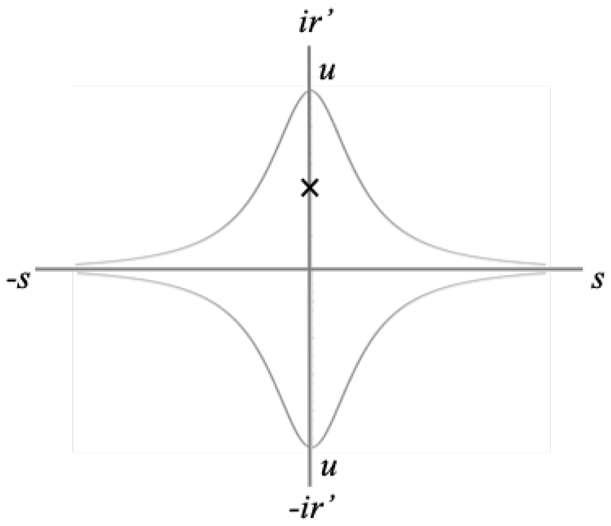
Note that D will range from 0 at to 1 at . We can plot the relationship between D and on the complex plane in Figure 13 for both the Universe and anti-Universe (we choose units where here so that the magnitude ranges from 0 to 1):
The two Universes are coincident at i, representing the event horizon/Big Bang era (in the rest of this paper, the Big Bang will be referred to as Annihilation). Here, we can say the matter and antimatter of the two Universes have annihilated with each other and new pairs of matter and antimatter filled Universes are created from the annihilation, creating the two Universes travelling in opposite directions of time. Over time, the imaginary radii of the Universes decrease while the real diameters increase up to the singularity, where the imaginary radii are 0 and the magnitude of the real diameters are 1.
The anti-Universe moves in the opposite direction of time relative to the Universe, and so we expect their vectors on this plane to rotate in opposite directions as shown.
Looking at Figure 13, we can mirror the curves in the real axis to account for the space. Doing so would indicate that right as the Universes reach maximum expansion, the geodesics reverse in time and the Universes begin to re-collapse toward each other until they collide once again and annihilate.
11. Newtonian Analog
This entire system is the temporal equivalent of two masses initially moving apart from one another until they reach a maximum separation distance u. At that point they will start falling toward each other again due to mutual gravitational attraction. When they meet at their common center, they annihilate, creating new pairs of matter/antimatter particles and begin moving away from each other again, as if they’ve bounced off each other. It is equivalent to the exchange of potential and kinetic Energy, but in the time dimension.
Now consider the Newtonian example of a ball in a gravitational field rising to a maximum height h and then falling back to the ground. will be positive on the way up, negative on the way down and zero at max height. But this also means that will be infinite at the maximum height because there. We might think that when comparing this to the present case, and , but this is incorrect. We know that r is our time coordinate and is the distance along the geodesic, so and . So from Equation (11), we see that, just like in the Newtonian example, and at the singularity because in this case at the turnaround.
12. Condensation and Evaporation
We will now describe in detail the physical meaning behind the ’Expansion’ and ’Collapse’ phases of the Universe. Looking at Equation (13), we see that the term is always positive. During the expansion phase, is negative and therefore will always be in the opposite direction of . Therefore, this tells thus that the peculiar velocities of cosmological objects will be reduced over time when no forces act upon them. Equation (13) describes an inertial force acting on all objects, slowing them down during the expansion phase. If the Universe is far from and , it only has noticeable effects at very large time scales and velocities (because is very small for human velocity and time scales. For instance, currently so converting that to gives a value on the order of ). During collapse, is positive and now the acceleration acts in the direction of motion of the object and therefore increases its velocity over time in that phase.
So we can view the expansion phase as a condensation of the Universe. The Universe starts out as a hot plasma after the annihilation event, after which it cools and motion of the particles slow down. At the beginning of expansion, the deceleration is large (infinite at allowing null geodesics to become timelike), then for a long period the deceleration is small, and on approach to the signularity it once again goes to infinity. For just a moment at the singularity, all motion stops completely. The particles stop completely at the singularity because , and therefore become infinite there putting an infinite inertial drag force on all objects. This is true even for objects with a proper acceleration. So the expansion counter-intuitively effectively stabilizes gravitational structures more and more as time moves forward, promoting this condensation.
Likewise, the collapse phase can be viewed as an evaporation. After condensation, the Universe begins the collapse phase. As the Universe emerges from the singularity, the inertial force that now tends to accelerate is extremely large (falling from infinity at the singularity), but the of everything is zero, so there is no initial acceleration at the very beginning of collapse. But any perturbation to a particle’s state of rest will induce an inertial acceleration in the direction of motion. Therefore, particles will naturally gain momentum over time and the Universe will heat up as gravitationally bound structures begin to break down and the Universe tends back toward a state of hot plasma as it approaches the annihilation event. Once again , and therefore become infinite at the annihilation event, sending all particles toward light-like geodesics as though they effectively lose all their mass.
Now let us consider this from the perspective of the external metric. Consider a star that has collapsed to form a Black Hole. As will be demonstrated, the star can never actually form an event horizon, but we can imagine that the star is massive enough that it becomes a ’Dark Star’.
The Schwarzschild metric depicted in Figure 1 describes an ’eternal’ Dark Star. But we could also say that it describes a Dark Star from the beginning of the Universe to the end of the Universe, with the beginning of the Universe being marked by the line and the end being the line. The Schwarzschild metric is asymptotically Minkowskian, so it does not truly represent the spacetime around a real spherically symmetric mass since the background Universe has been observed to be non-Minkowskian, but we can use this metric along with what has been determined from Equation (13) to approximate the expected trajectory for a freefalling object in the field of a Dark Star over the expansion and collapse phases of the Universe. The path of an object in freefall in the field of a Dark Star as seen by a distant observer is given by [7]:
Where is the radius at which the object begins falling from rest and is the Schwarzschild radius. The focus here is not on the equation itself, which is a well-known solution, but at the ± in front of it that comes from taking the square root. We first note that in the external metric is the proper time interval of an observer at infinity. In the cosmological case, this interval is the proper time of the co-moving observer . Therefore, we can modify Equation (41) as follows:
For an observer falling in the external metric from some , is always positive. But we know that is negative during expansion and positive during collapse. Therefore, if we take the positive root of Equation (42), we see that during expansion will be negative (because is negative) and during collapse will be positive. We assert that the time at which the Universe changes from expansion to collapse is at and therefore the expansion occurs in the region and collapse occurs in the region.
So during collapse, freefalling objects are ejected symmetrically out of the gravitational field of the object relative to expansion. We also note that at , and therefore . So we can say that as an object approaches , its worldline must become tangent to the hyperbola closest to it. And as collapse begins, it will smoothly and symmetrically curve in the opposite direction. Furthermore it should be noted that since the expansion phase takes place in the region, an event horizon can never form because that would require faster than light motion to achieve.
An approximate example of a real geodesic for an object in freefall in such a gravitational field is shown by the dark black line in Figure 14 through both the expansion and collapse phases of the Universe.
The conclusion we can draw from this is as follows. During expansion, the background of the Universe glows with decreasing temperature and brightness over time via the CMB as gravitational structures stabilize and galaxies form. During this phase, some stars will collapse to form Dark Stars that we presently think of as Black Holes. By the time we reach the singularity, the Universe will be fully condensed and inert. At the singularity, light from the CMB will be infinitely redshifted such that it is no longer detectable and the background Universe becomes black (because in Equation (15) becomes infinite there). The observer will see a completely dark Universe at the singularity and over time, the Dark Stars will begin to glow like candles lighting up the darkness as the geodesics of the particles that were falling toward their centers during expansion reverse and now move outward (unabsorbed light will also be reflected back outward during collapse). Shadow becomes flame. These former “Black Holes” effectively become “White Holes”, with matter radiating from them, seemingly out of the vacuum, even though the radiation is coming from matter that had accumulated in that region during expansion. As the collapse proceeds, these White Holes will grow brighter and shrink as the matter and energy making them up escapes to the external Universe at higher and higher energies due to the increasing inertial acceleration from Equation (13). The Universe effectively evaporates as all gravitational structures break down. By the end of collapse, the Universe has returned to a state of increasingly dense plasma until it collides with the anti-Universe at the annihilation horizon.
We can summarize as follows: We know from Equation (13) that the worldlines of all matter become null at the end of collapse, so by symmetry, they will begin the expansion as null geodesics as well at . They enter the singularity parallel to the t coordinate per Equation (13) at the end of expansion. The geodesics then begin to move from to increasing r during the collapse (interpretation of the infinite curvature is given in Section 15), accelerating inertially over time per Equation (13). Observers are inertially accelerated to become null geodesics as they approach the annihilation event at the end of collapse per Equation (13).
Note that if the Universe collapses over the same manifold on which it expanded, this would suggest we live in a ’presentist’ Universe as opposed to a ’block’ Universe because if that were not true, the collapsing matter would collide with the expanding matter.
13. Total Proper Time
The proper time in Equation (1) implicitly assumes the local gravitational field is in a co-moving cosmological frame. This is because must be a function of cosmological time r. In fact, we know that as the proper time interval of the co-moving observer has to be equal to the interval, we can choose to be . But there is no reference to the spacelike t and cosmological dimensions in the internal metric. If the source of the gravitational field has cosmological motion, the true proper time will be reduced relative to Equation (1) due to time dilation effects. The total proper time interval is found by multiplying by the ratio of for the actual cosmological motion of the field source and of a co-moving frame:
Which becomes:
Recognizing that is the linear cosmological speed of light (Equation (12)), we can define and the cosmological linear speed of light . We also define the angular speed and the cosmological angular null geodesic as (by solving for in Equation (2) with ), then we can write Equation (44) as:
If we multiply by , and recognize that is the total cosmological velocity (because is the tangential velocity which is perpendicular to the linear velocity), then we recover the Minkowski form of the length contraction equation where the speed of light varies over cosmological time:
This is telling us that the worldlines in metrics such as the external Schwarzschild metric are contracted by the system’s cosmological motion. So we see that the cosmological model is essentially a collection of systems described by metrics like the external Schwarzschild metric in a hyperbolic background that is a quasi-Minkowski metric with a time dependant speed of light.
In order for Equation (45) to be real, the quantity under the square root must be positive and therefore
And so we see that the upper speed limit of an object depends on its spin. In other words if and object is spinning about the time dimension while moving in a straight line, its maximum speed will be reduced per Equation (47). It’s as though this spin has increased the mass of the particle, and perhaps even gives mass to a massless particle. The mass would be related to the precession of the inertial frame about the time axis.
14. ’Spaghettification’, and a Self Portrait of the Universe
We will now take a closer look at what actually happens at the singularity in the cosmological context. When approaching the singularity, the term vanishes and proper distances go to infinity. This is often referred to as ’spaghettification’. In the conventional context of falling into a Black Hole, this is interpreted as an observer approaching the singularity getting both infinitely stretched and squeezed and then they just cease to exist at the singularity. But when we interpret the internal metric as the cosmological solution, we find that the true nature of the metric behavior at the singularity is in fact much more mundane, yet incredibly revealing.
Let us now consider the singularity. The light cone opening angle at a given cosmological time is given by:
Figure 15 shows the light cone angle as function of r as we move along the r axis with decreasing r during expansion, through the singularity, and then in increasing r during collapse.
We begin expansion at the left side of the diagram where the light cone is totally open (), because Equation (12) goes to ∞ there. As we move through time, the angle closes until at the singularity, light no longer travels through t (), which is why Equation (12) goes to zero there. At the singularity, light no longer travels through space and everything becomes spacelike. But also recall that motion has stopped at this point and all light is infinitely redshifted, so there isn’t really a physical stretch happening, its only that adjacent points in space are unable to communicate with each other at that instant. Then as we pass the singularity and continue moving now with increasing r during collapse, the light cone will start opening in a symmetric way to how it closed during expansion.
Therefore, space is not expanding the way we currently think about it in terms of a stretching of space. What is changing is how quickly different points in space are able to communicate with each other. The image of space itself compressing to a point or ripping itself apart is misleading. At the beginning of expansion, we have a normal 3D space of particles that can communicate instantly with all other particles regardless of distance because the speed of light is infinite there. This communication speed drops as expansion proceeds and local gravitational structures are able to form. When reaching the singularity where the scale factor is infinite, space is not ripped apart but rather the light cone angles have closed completely such that adjacent regions of space are unable to communicate with each other which manifests as infinite proper distances.
Finally, let us return to Equation (10) and track the proper distance s of a point a fixed coordinate distance t away from us for the duration of the expansion and collapse. If we plot this proper distance vs the imaginary version of similar to what was done in Figure 13, we get a clean picture of how the expansion and collapse of the Universe would appear to a co-moving observer (expansion and collapse proceeds from top to bottom). The reader’s current position is marked with ’x’:
Figure 16.
Self Portrait of the Expansion and Collapse of the Universe with the Reader’s Current Position Marked with ’x’.
Figure 16.
Self Portrait of the Expansion and Collapse of the Universe with the Reader’s Current Position Marked with ’x’.
Note that this is not the Universe and anti-Universe. When the Universe is at , that is where the Duoverse collides.
15. The Many Worlds
The Duoverse described thus far contains all the events in the Universe and anti-Universe for a single expansion from beginning to end. However, the Duoverse then re-collapses, annihilates, and pair produces a brand new Duoverse. Therefore, we can think of each successive expansion and contraction of the Duoverse as happening along another dimension which is discrete. This dimension essentially labels the different countably infinite random set of Duoverses.
Since each Duoverse begins with annihilation, this means each Duoverse begins with a random configuration after annihilation. Therefore, there is no cause and effect relationship between Duoverses from cycle to cycle. This means the cycles cannot be ordered sequentially because there is no way to know which cycle preceded or will follow the current cycle. If we cannot order the cycles in a sequence, then we can think of them all as being parallel to each other. While events within a cycle can have cause and effect relationships (i.e., the events ’happen’ at given times), the various cycles themselves do not ’happen’, they just exist along side all other cycles. Thus we can think of the annihilation events as being a single event from which infinite Duoverses emerge and to which they return. This implies that finding ourselves in a particular Duoverse is completely probabilistic where the probability that we find ourselves in a Duoverse with a particular configuration depends on how likely that configuration is across all possible configurations. This gives us the many worlds that have been invoked to explain quantum probability in the Everett many worlds interpretation of QM. The parallelism of the cycles also resolves the paradox that would come with infinite sequential cycles: If the Universes cycled in series, that would mean that an infinite amount of cycles would need to occur before our cycle, which is a logical paradox.
We can visualize the geometry of time with the many worlds and infinite curvature by imagining a 2D surface with a finite height and infinite width as shown in Figure 17:
We see both the Universe and Anti-Universe with normal vectors representing which side of the (infinitely thin) surface they are on (with matter pointing in one direction and antimatter pointing in the opposite direction). They move from to during expansion and vice versa during collapse along the dotted line on the surface. The curvature is infinite at and this corresponds to the normal vectors representing the Universes’ orientation relative to the surface flipping direction at that point. So we can imagine one vector pointing up and the other pointing down at the solid center line of the sheet, and as expansion progresses, these vectors are transported along the dashed line toward (moving in opposite directions). At , the vectors flip their directions and move back toward the center line during collapse (where the direction flip reflects the idea that the Universes are now on the opposite side of the surface they were on during expansion).
Each point on the dashed line maps to a 3D space representing the Universe or Anti-Universe at a specific time. The many worlds would be lines on the surface parallel to the dashed lines of Figure 17. There would be countably infinitely many such lines (i.e., this quasi-dimension is discrete where its coordinates is the set of integers, not real numbers), one for each of the infinite parallel Universes (this is why the width of the surface in Figure 17 is infinite). Thus, the width of the sheet would represent a kind of “possibility space”.
We can also think of this a in terms of an analogy between the galaxies in our Universe and the many worlds. If we consider an ideal galaxy, the center of the galaxy has an event horizon which looks like a surface from far away but is a point of infinite coordinate density when it is approached. This would correspond to the Big Bang/annihilation event of our Universe. Near the event horizon at the galactic center, we have a hot accretion disk made up of very high momentum particles. This would correspond to our Universe before recombination when the Universe was a high-temperature plasma. As we move out radially from the galactic center, the density of stars and gas drops at greater and greater radii. This corresponds to the post recombination era of the Universe where the matter density goes down as time passes. As we move very far from the galactic center, the mass density drops to zero and we just get empty space. This would correspond to approaching the singularity in the internal metric where the proper distances go to infinity and the spatial coordinate density of the vacuum goes to zero. And we can think of the infinite different galaxies separated in space in our Universe as being equivalent to the many worlds described above separated in time but existing in parallel with our Universe. So we can imagine moving radially in a straight line from one galaxy to another. Moving from the center of the first galaxy to the vacuum between the galaxies would correspond to the expansion phase of the Universe and then moving from the vacuum to the center of the second galaxy would correspond to the collapsing phase. Keep in mind that the hypothetical event horizons at the center of every galaxy correspond to the same point since it is the location in spacetime where all space is collapsed (this is even true in the external metric where looking at Figure 1, the horizon is a and all the r hyperbolas are coincident when ).
But perhaps Figure 17 is too simplistic. Maybe our 4D spacetime is not naturally described in the Cartesian basis of Minkowski spacetime. Perhaps the spacetime is better understood as having two directional dimensions described with along with a complex linear dimension (a complex radius) of real space and imaginary time (i.e., the form of the Schwarzschild metric). Perhaps beyond the future singularity, when our Universe will reverse its direction in time, lie the countably infinite many world Universes in all directions of the timelike dimension, scattered throughout an “Omniverse” just like the galaxies that permeate the space in Universe we know. And looking at Figure 2, we note that the null geodesics (45 degree lines) can in theory extend beyond the hyperboloid (pictured there) in the T (vertical) direction such that perhaps during the collapse phase, instead of the CMB being the background of the Universe, observers there would see escaped light from these other Universes in the unreachable distant sky.
We can formalize this a little more by simply allowing r to be negative. It was always assumed that r could not be less than zero because represented the center of a Black Hole, but as this paper demonstrates, this is not the case. So substituting into Equation (2) we get:
We put values of into this metric since we’ve already absorbed the negative sign into the equation. This once again looks (somewhat) like the external metric with the t coordinate being timelike and the r coordinate being spacelike, but has characteristics of both the external and internal metrics. In this metric, this ’outer-spacetime’ geometry on the Kruskal coordinate chart is a 2-sheeted hyperbolid as opposed to the 1-sheeted hyperboloid geometry of the external metric. But we note that like the external metric, as , the metric also becomes Minkowskian. Also note that in this metric, similar to the internal metric, u merely sets the units of space for the metric.
Interestingly, in this outer-spacetime, our Universe (and potentially all the infinite Universes) will look like a kind of point-like Black hole because no matter inside of it would be able to escape due to the infinite curvature at (the turnaround point from the perspective of our Universe). Note that, apart from , there are no singularities in this metric, and therefore there are no event-horizon-equivalent locations in the spacetime. We can also see that light comes out of these points with infinite and slows to as .
So for an observer in this outer-spacetime, Universes would look like points of light scattered throughout the spacetime. If light is allowed to escape the Universes, the specific photon from the Universe that they would see in the outer-spacetime would depend on their location and time in the outer-spacetime. But if light from within the Universe cannot escape, then perhaps the points are blackbody points radiating at the temperature of the Universe at various times.
This is mostly speculation at this point, but future research may be able to put such a hypothesis on more solid footing.
Data Availability Statement
All data generated or analysed during this study are included in this published article [and its supplementary information files].
Conflicts of Interest
There are no competing interests.
References
- Raine, D.; Thomas, E. Black Holes a Student Text; Imperial College Press, 2015.
- Carroll, S.M. Lecture Notes on General Relativity. arXiv 1997, arXiv:gr-qc/9712019v1.
- Lima, J.A.S.; Jesus, J.F.; Santos, R.C.; Gill, M.S.S. Is the transition redshift a new cosmological number? arXiv 2014, arXiv:astro-ph.CO/1205.4688.
- Bond, H.E.; Nelan, E.P.; VandenBerg, D.A.; Schaefer, G.H.; Harmer, D. HD 140283: A Star in the Solar Neighborhood that Formed Shortly after the Big Bang. Astrophys. J. 2013, 765, L12. [Google Scholar] [CrossRef]
- Supernova Cosmology Project - Union2.1 Compilation Magnitude vs. Redshift Table (for your own cosmology fitter). 2010. http://supernova.lbl.gov/Union/figures/SCPUnion2.1muvsz.txt. (accessed on 17 August 2017).
- Risaliti, G.; Lusso, E. Cosmological constraints from the Hubble diagram of quasars at high redshifts. arXiv 2018, arXiv:astro-ph.CO/1811.02590.
- Augousti, A.; Gawełczyk, M.; Siwek, A.; Radosz, A. Touching ghosts: Observing free fall from an infalling frame of reference into a Schwarzschild black hole. Eur. J. Phys. 2012, 33, 1–11. [Google Scholar] [CrossRef]
| 1 | Figures 1, 4, 10, 12 and 14 are modifications of: ’Kruskal diagram of Schwarzschild chart’ by Dr Greg. Licensed under CC BY-SA 3.0 via Wikimedia Commons - http://commons.wikimedia.org/wiki/File:Kruskal_diagram_of_Schwarzschild_chart.svg#/media/File:Kruskal_diagram_of_Schwarzschild_chart.svg
|
Figure 1.
Kruskal-Szekeres Coordinate Chart.
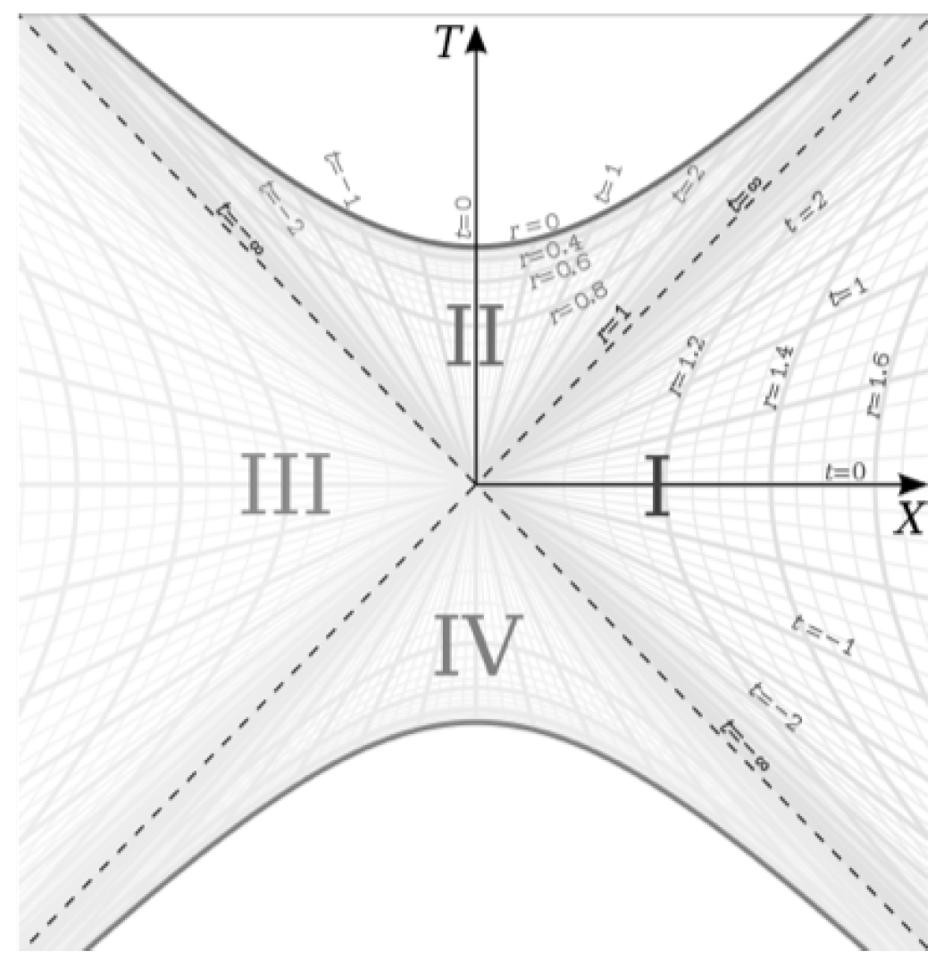
Figure 2.
2D Surfaces of Constant r for Internal and External Metrics.
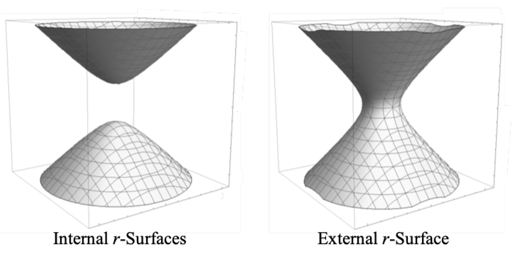
Figure 3.
Killing/Basis Vectors on a Surface of Constant r.
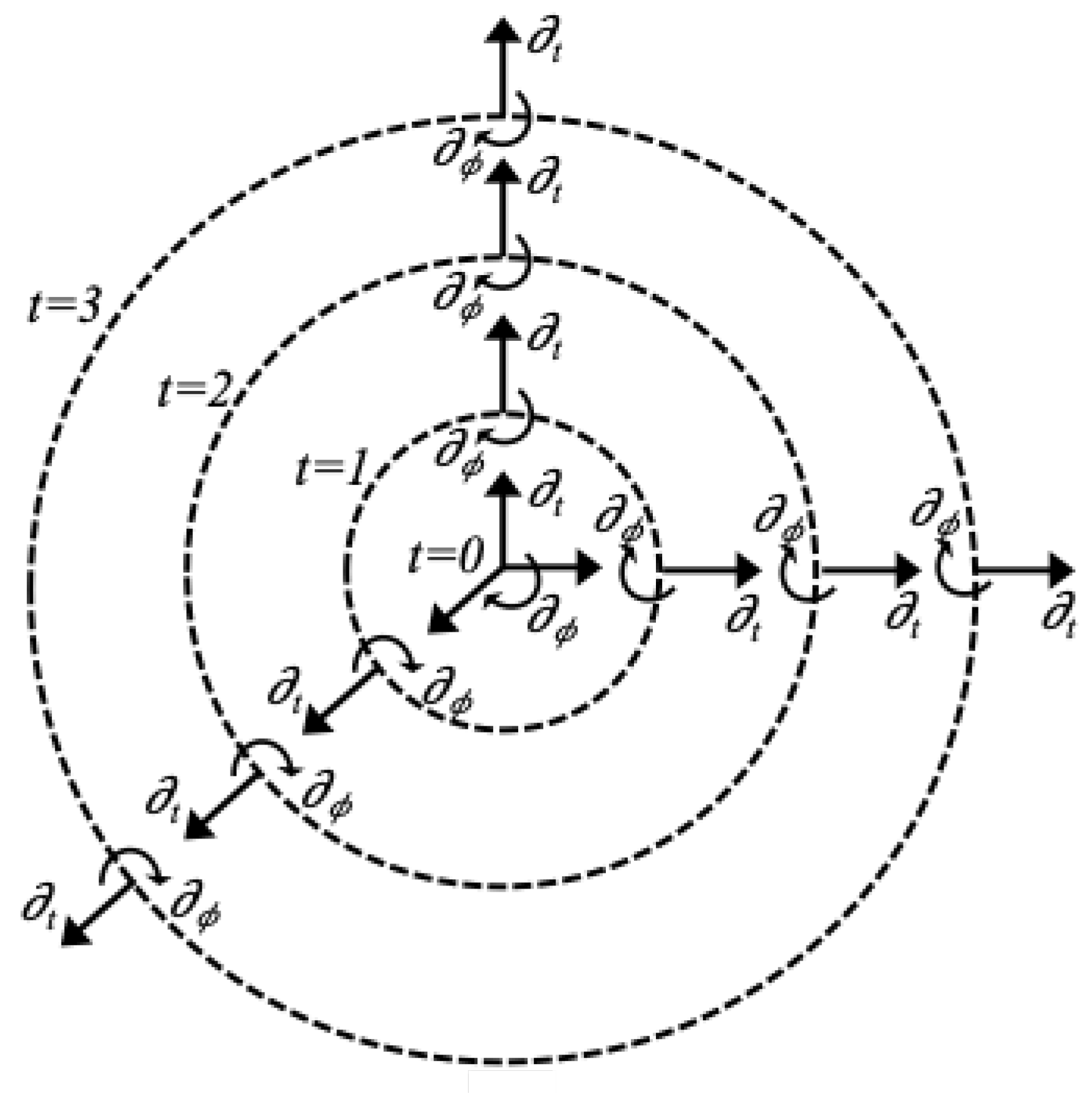
Figure 4.
Projection of the Past Light Cone on a Flat Plane.
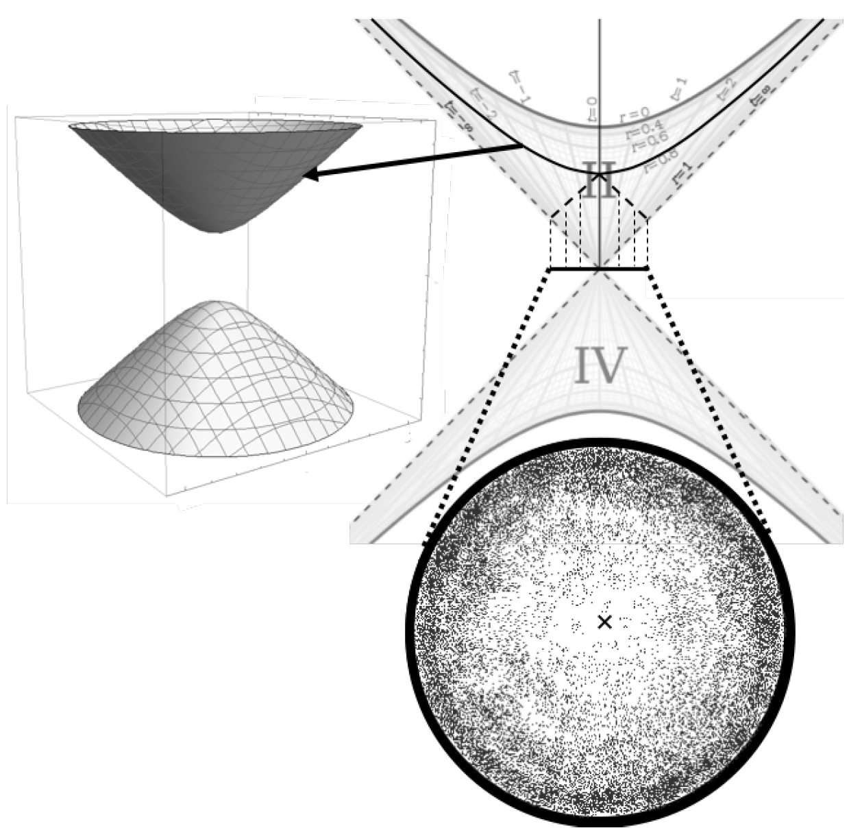
Figure 5.
Scout and Jem on a Collapsing Shell.
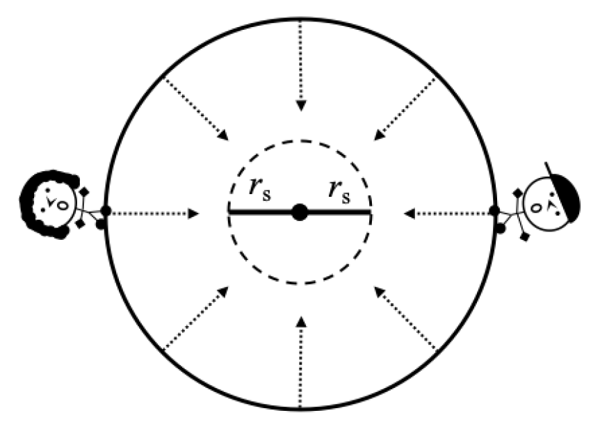
Figure 6.
Scale Factor vs. r for .
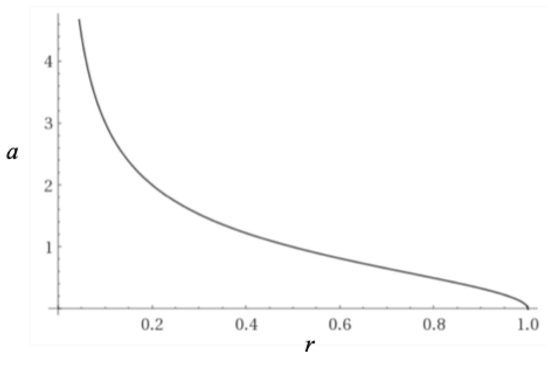
Figure 7.
Distance Modulus vs. Redshift Plotted with Supernova Measurements.
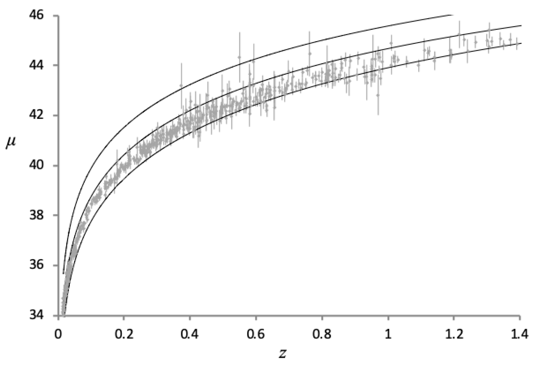
Figure 8.
Distance Modulus vs. Redshift Plotted with Quasar Measurements.
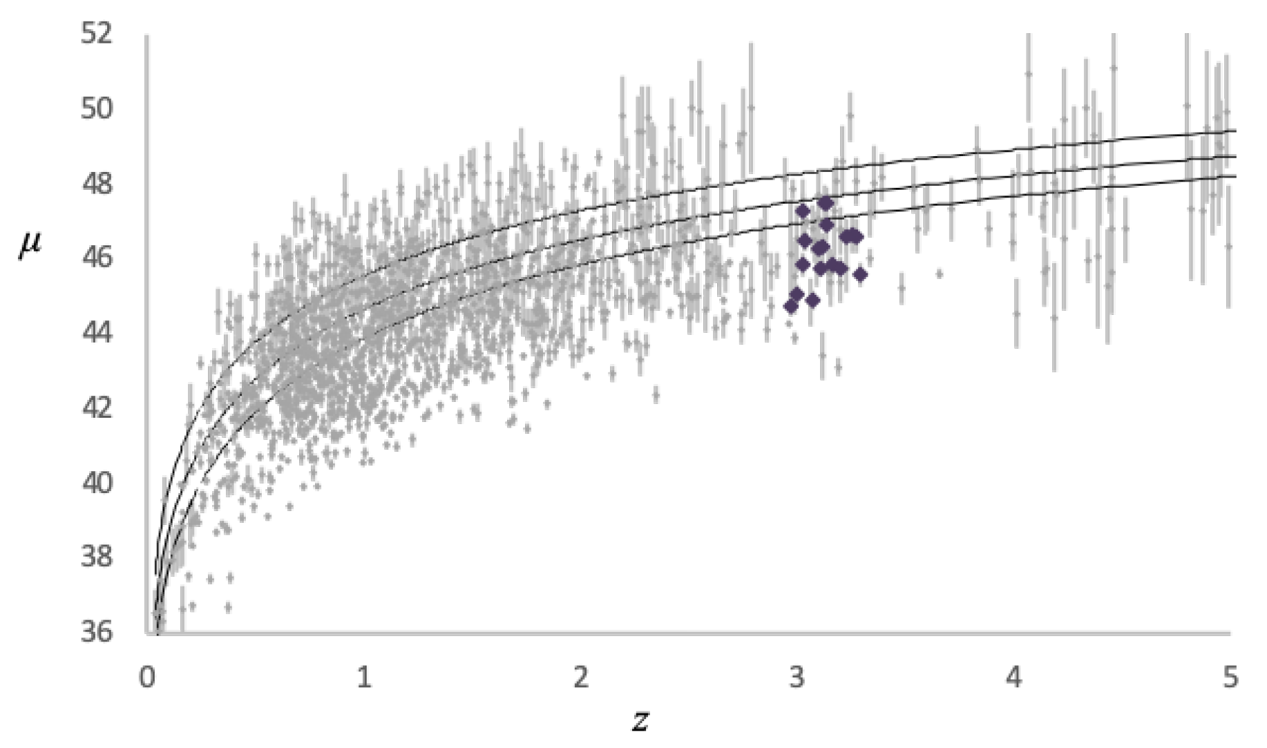
Figure 9.
Lookback Time vs. Redshift.
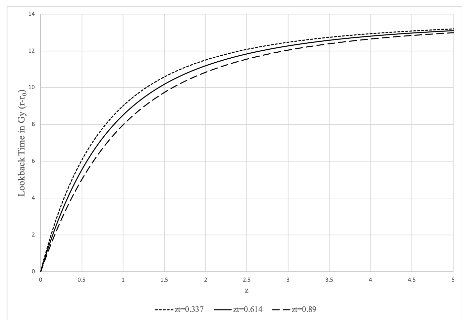
Figure 10.
Depiction of Linear Cosmological Motion.
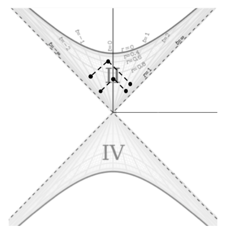
Figure 11.
Visualization of Circular Orbit.
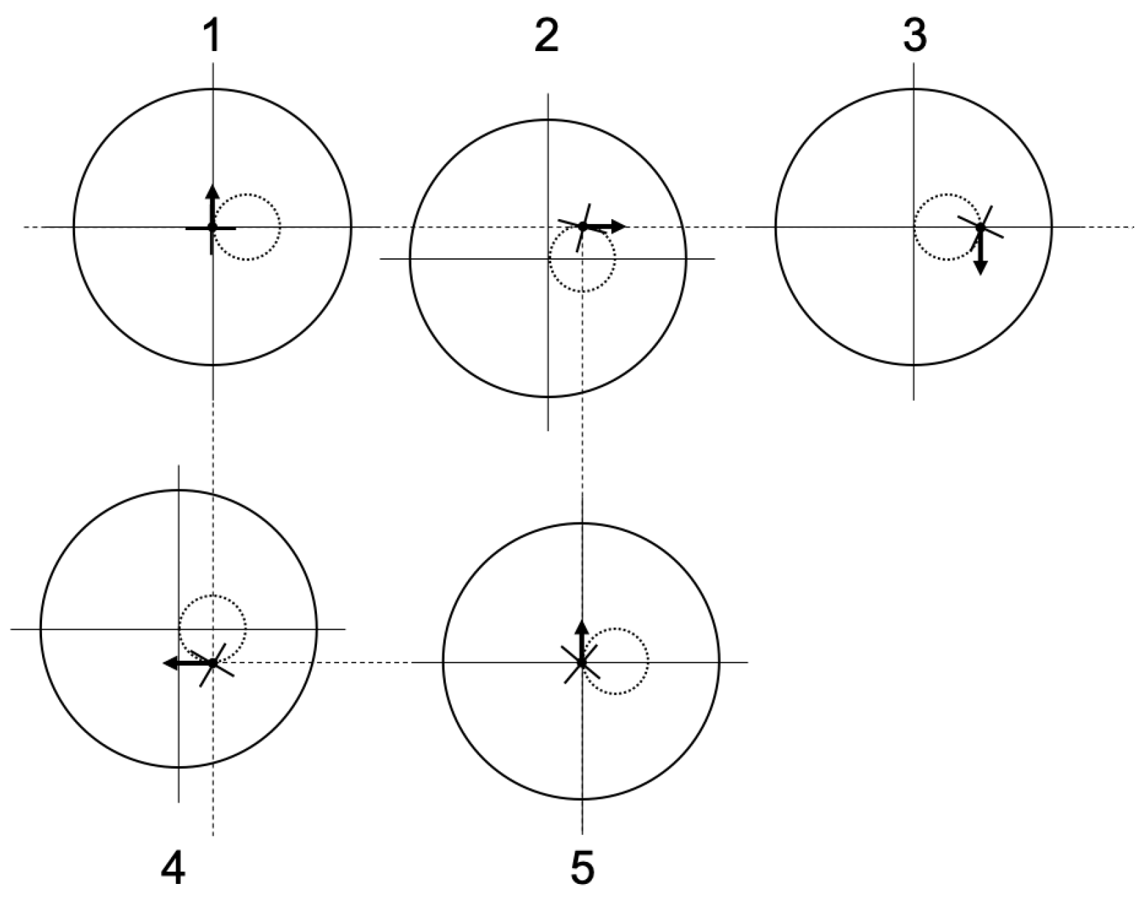
Figure 12.
Universe and Anti-Universe.
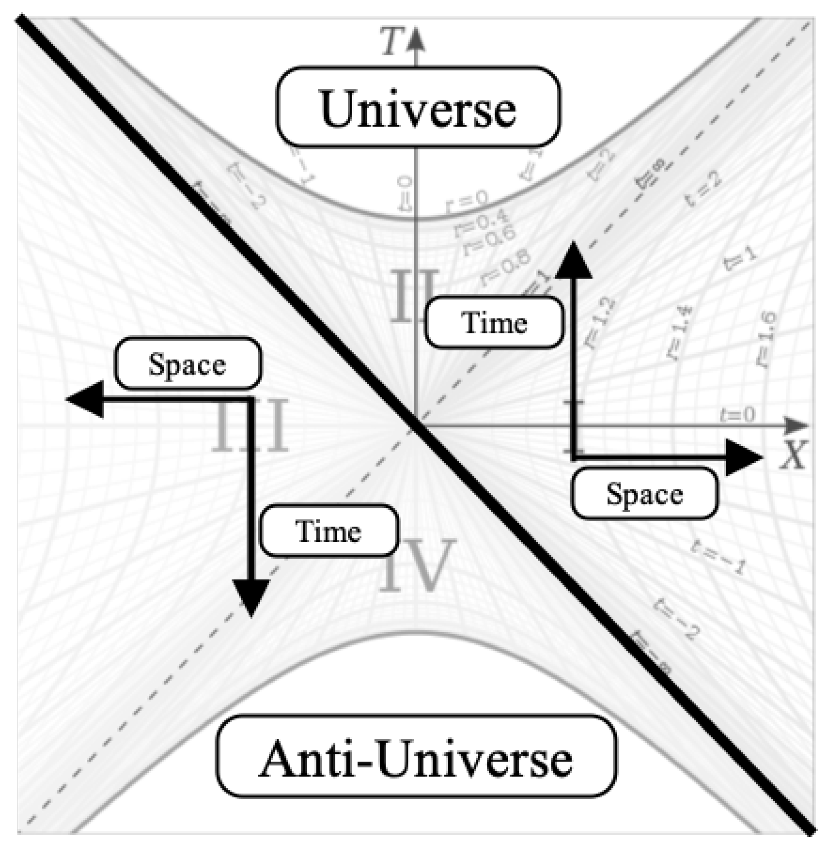
Figure 13.
The Universe (Right) and anti-Universe (Left) in the Complex Plane.
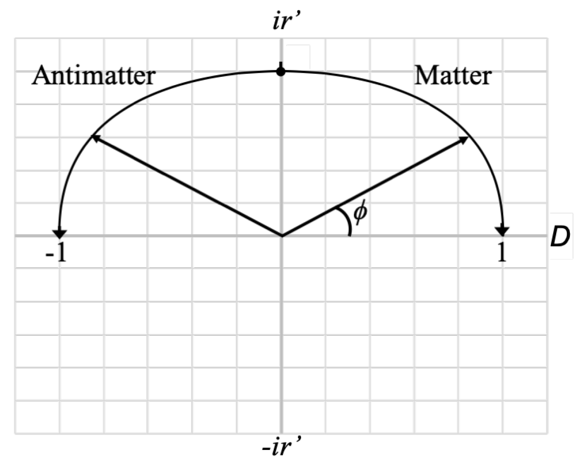
Figure 14.
Schwarzschild Freefall in Expanding and Collapsing Spacetime.
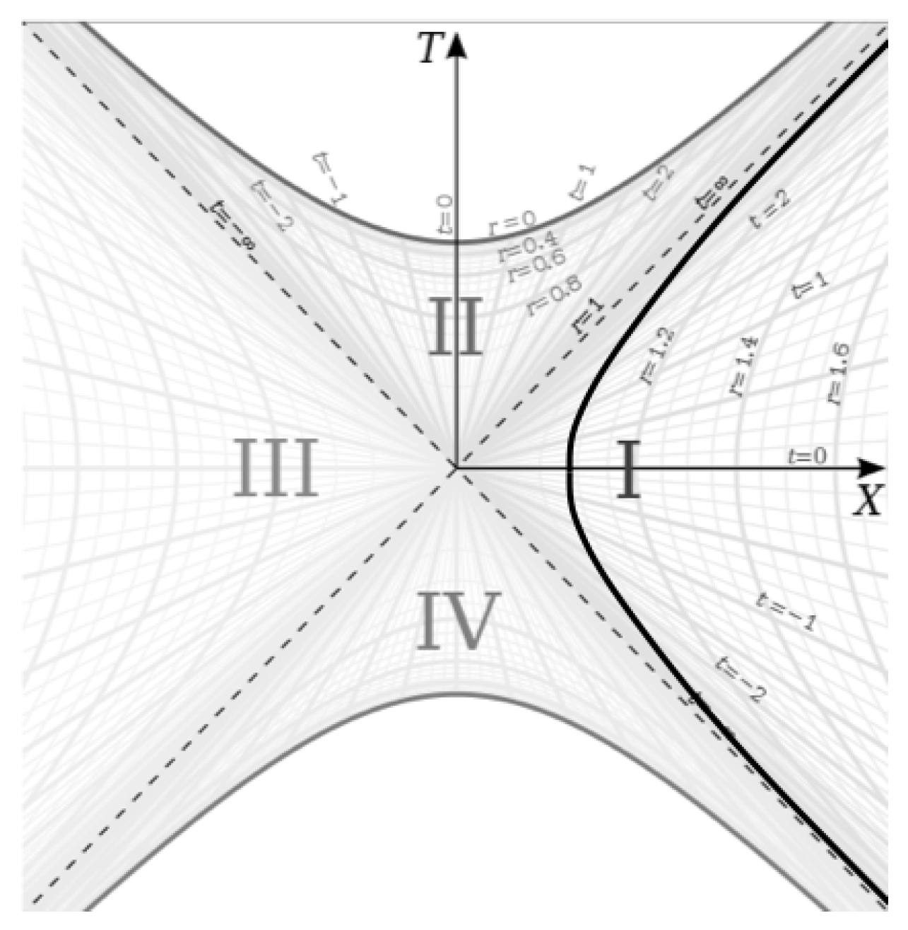
Figure 15.
Local light cone angles over time.
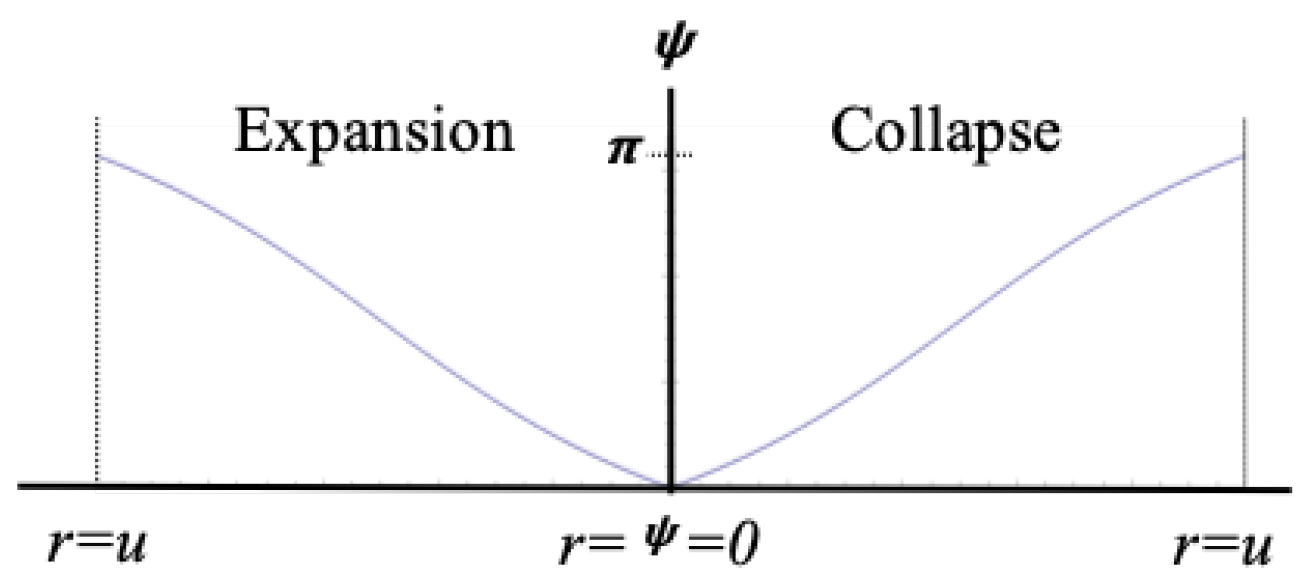
Figure 17.
The Many Worlds Parallel Time Surface
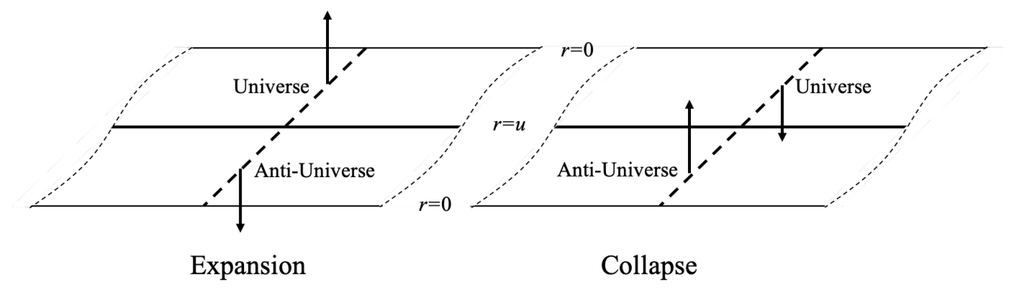

Table 1.
Limiting Cosmological Parameter Values Based on Measurement and a 13.8 Gy Age of the Universe.
Table 1.
Limiting Cosmological Parameter Values Based on Measurement and a 13.8 Gy Age of the Universe.

Table 2.
Limiting Proper Times Based on Measurements and an age of 13.8 Gy for the Universe (Time is in Gy).
Table 2.
Limiting Proper Times Based on Measurements and an age of 13.8 Gy for the Universe (Time is in Gy).
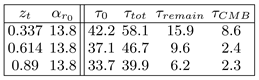
Disclaimer/Publisher’s Note: The statements, opinions and data contained in all publications are solely those of the individual author(s) and contributor(s) and not of MDPI and/or the editor(s). MDPI and/or the editor(s) disclaim responsibility for any injury to people or property resulting from any ideas, methods, instructions or products referred to in the content. |
© 2023 by the authors. Licensee MDPI, Basel, Switzerland. This article is an open access article distributed under the terms and conditions of the Creative Commons Attribution (CC BY) license (http://creativecommons.org/licenses/by/4.0/).
Copyright: This open access article is published under a Creative Commons CC BY 4.0 license, which permit the free download, distribution, and reuse, provided that the author and preprint are cited in any reuse.