

Submitted:
07 August 2026
Posted:
11 August 2026
You are already at the latest version
Abstract
We developed a formulation of classical electrodynamics in the 2T + 3S dimensions without compactifying the extra time dimension. We found an effective electric charge defined by the ratio of the two distinct speeds of causality. We extended the concept to the hadronic Color-Space and postulated that the massless gluon was tied to the second time dimension, with an intrinsic speed different from the speed of light. We applied the theoretical formulations to the e+e- → hadrons experiments and suggested a preliminary estimate of the gluon speed using the R- values.
Keywords:
extra time dimension
; classical electrodynamics
; QCD
; R-values
; gluons
1. Introduction
Recently, Zahir [1] considered a two-time (characterized by distinct causality speeds c1 and c2) and three-space-dimensional Minkowski space (2T + 3S). He derived relativistic coordinate and velocity transformation formulas and expressions for a new effective speed limit where k is a scale factor connecting the two times t1 and t2. If dimensions of t1, t2, and any of the space dimensions are denoted by T, t, and L, respectively, then dimensions of c1, c2, and k are LT-1, Lt-1, and Tt-1, respectively. We emphasize that although t1 and t2 are both “time-like” variables, this time (t1) is not the same as that time (t2). Previously, Velev [2] explored the formulations of coordinate and kinematic transformations in a detailed analysis of a flat space-time with extra time dimensions. However, Velev [2] used the same speed of causality c for all time dimensions, including the extra ones. This at least creates one calculational problem – we cannot take the limit for c assigned to the extra times to zero to get back the familiar four-dimensional (i.e., those of Einstein’s Special Theory of Relativity ([3] and references therein)) formulations in the Minkowski ([3] and references therein) space meaningfully. There was no way to distinguish one c from the other [2].
In our familiar space-time structure, the extra time dimensions are not observed, and thus, in all higher-dimensional physics, the idea of compactification has often been considered ([4,5] and references therein). Zahir [1] also discussed compactification in a two-time-dependent Schrödinger-like equation with an infinite square-well potential. After compactifying the extra time dimension on a closed-loop topology with a period matching the Planck time, the solution generated interference among additional quantum states with ultra-short oscillation periods as well. Zahir [6] also considered compactification in another related work on the Klein-Gordon-type equation in 2T + 3S dimensions. Tyagi and Al-Shahristani [7] developed the Dirac equations within Zahir’s paradigm but did not consider compactification of the extra time dimension.
In this paper, we will explore the extension of classical electromagnetic fields in the 2T + 3S dimensions without compactification. We will investigate how Maxwell’s equations are modified, if at all, in the five-dimensional “Lorentz” covariant analysis and its possible implications. We will postulate a bold physical space-time environment defined by two times related to two interactions carried by two massless intermediaries with two distinct speeds of causality. This is exactly the conceptual framework on which Zahir [1] developed his two-time relativity. The outcome will be intriguing as we relate it to experimental results from contemporary physics (see Section 4 and Section 5).
In Section 1, we introduce the concept of Zahir’s 2T paradigm [1] and a bold proposition of the Color Space (CS). In Section 2, the structure of the 2T +3S dimensional space is briefly reviewed. Section 3 is dedicated to developing formulations of classical electrodynamics, modified Maxwell’s equations, and the concept of effective charge in the 2T + 3S dimensions following a covariant approach. In Section 4, we present and extend the concepts of the 2T paradigm in the Color Space, with the massless photon and gluon mediating two interactions that move at two intrinsic speeds of causality. In Section 5, we use the experimental R-values of the e+e- → hadrons collision to derive a possible value of the gluon speed considering the effective charge. Conclusions and discussions are presented in the last Section.
2. Summary of the 2T + 3S Space-Time Structure
As noted earlier, the different speeds of causality for times t1 and t2 are given by c1 and c2. Thus, the space-time variables in the (2T + 3S) space are (). We consider Minkowski-like flat space with metric signatures (+, +, -, -, -) such that the invariant space-time interval ds is given by.
After a detailed calculation, Zahir [1] derived the 2T relativistic coordinate transformation for the reference frame K’ moving at a uniform speed relative to reference frame K. He considered the standard configuration, and the motion of K’ is along the x coordinate only, such that at t1 = 0 and t2 = 0, the coordinate axes of K and K’ coincide. K’ is moving with uniform velocities v and w defined with respect to times t1 and t2, respectively. So, if x0 is the coordinate of the origin of K’ with respect to K at any time,
This implies that. The expressions for coordinate transformations are given in equation box (1) below. For the full definition and expressions of the five-dimensional proper time, five-velocities, five-momenta, and various invariant relationships, see ref. [1].
3. Electromagnetic Field Tensors in the 2T + 3S Dimension: The Modified Maxwell’s Equations
3.1. The Electromagnetic Field Tensors
We begin our work with the familiar antisymmetric electromagnetic field tensor as defined in terms of the scalar and vector potentials [8,9], . In the 1T + 3S space-time (i.e., the four-dimensional Minkowski space), the four components of Aµ are φ and -Ᾱ for the time component and three space components, respectively (we use bold notations (or with a bar on top) for three-dimensional vectors). In our 2T + 3S space-time, we need to propose an intuitive ansatz for the second component, A2, of the five-potential. Note that for the extra time dimension t2, we assumed . For A2, we assume and h is an unknown dimensionless parameter. We will see later what value for h will restore consistency with the familiar form of Maxwell’s equations. Therefore,
Out of 25 elements of the antisymmetric tensor, 10 are independent. We recall the following notations before proceeding to compute the 10 elements presented in Table 1.
While deriving the tensor elements, our inputs are the components of Aµ, and we will define the traditional relations and. We could have used any other symbols in place of E and B (say, P and Q), and the resulting equations would involve P and Q. However, at the end, we will need to identify them as E and B to make the equations consistent with the familiar Maxwell’s equations. Fµν can be represented in the matrix form (µ and ν are row and column indices respectively),
Later, we also need Fµν = . It can also be derived directly from Fµν as follows,
Fµν can also be represented in matrix form after doing the matrix multiplications using (2) and
Finally, we get
Restoring all values, we get the explicit expressions for the relevant elements of Fµν in Table 2.
3.2. Deriving Maxwell’s Equations from the Electromagnetic Field Tensors in the 2T + 3S dimension: The Covariant Approach
Here, λ, µ, and ν are all different, with possible values (1, 2, 3, 4, 5) for each. It is worth noting that the field tensors Fµν are antisymmetric and thus the diagonal elements are zero. There are 60 nonzero equations that can be divided into 10 sets of 6 each. The members of each set are different permutations of the indices and are the same except for an overall sign. Since the right-hand sides of the equations are zeros, the sign does not matter. There are 10 unique equations representing each set.
We denote the sets as
A: {λ, µ, ν} → {1,2,3} implying 1,2,3; 1,3,2; 2,1,3; 2,3,1; 3,1,2; 3,2,1
B: {λ, µ, ν} → {1,2,4} C: {λ, µ, ν} → {1,2,5} D: {λ, µ, ν} → {1,3,4}
E: {λ, µ, ν} → {1,3,5} F: {λ, µ, ν} → {1,4,5} G: {λ, µ, ν} → {2,3,4}
H: {λ, µ, ν} → {2,3,5} I: {λ, µ, ν} → {2,4,5} J: {λ, µ, ν} → {3,4,5}
The details of the calculations are given in Appendix A. We present the results,
Three equations representing A, B, and C are identically zero.
Three equations representing D, E, and F combine to give
Three equations representing G, H, and I combine to confirm
The equation representing J gives,
Here we used the traditional relations,
Next, we explore inhomogeneous equations involving sources. They can be derived from the covariant form,
Again, we need to make an ansatz regarding the second component of the charge-current five-vector J’ν,
where r is a dimensionless quantity (like h) that will be determined later. We will use the five-dimensional Lorentz condition to decouple the equations. For a full expression of the Lorentz condition in five dimensions, see Appendices B, C, D.
- (1)
- ν = 1
The corresponding equation is,
- (2)
- ν =2,
We can get an interesting result if we substitute Equation (4) in Equation (3) and use Equation (2), in which
items with a bar on top are three-dimensional vectors corresponding to the space coordinates (3), (4), and (5). See the detailed calculations in Appendix C, and we get,
Using the Lorentz condition , we get,
which simplifies Equation (4) to
- (3)
- ν = 3, 4, 5
Using in the equation above, we get,
In Equation (6), we substitute and expand as usual.
Using Equation (2) and , we get,
It is a decoupled equation as in four-dimensional electrodynamics. See Appendix D for the detailed calculation. We can also derive the continuity equation by applying on both sides of Equation (6), and using Equation (3) and Equation (5) and simplifying the tedious calculations (see Appendix E),
we get,
It is worth noting that, so far, we have derived one condition: r = h. However, if we set,
the Equations (3) and (6) become more like the familiar four-dimensional ones,
Equation (7) remains unchanged. Let us explore Equation (8).
Let us define
Then, the Equations (5), (9), (10), and (11) can be rewritten as,
If we integrate
over the space volume, we get,
In summary, the new formulations are very similar to the corresponding Maxwell’s equations in four dimensions. The effect of the extra time dimension (albeit subject to the various ansatzes) is that it gives us an effective electric charge,
In addition, the wave equations, the continuity equation, and the Lorentz condition are extended to five dimensions. We will use these theoretical results in the context of a new, intriguing proposal regarding two-time physics with different speeds of causality. We present it later in Section 4 and Section 5.
2. Conceptualizing the Segmented Space-Time of Photons and Gluons: A Bold Proposition
In [1], Zahir presented a conceptual framework for a 2T + 3S-dimensional spacetime in which two interactions are mediated by two massless particles moving at two distinct speeds of causality, c1 and c2. Applying the principles of the Special Theory of Relativity (STR) to the expanded space-time, we can formulate it in terms of the following “gedanken” scenarios [1].
Let us denote the interactions as I-1 and I-2. First, we turn off interaction I-1 and consider a space-time structure with 1T + 3S dimensions, where interaction is carried by a massless particle moving with speed c1 (i.e., the speed of causality). Therefore, the space-time transformations (think STR) between inertial reference frames will be the Lorentz transformations ([10] and references therein) with. Then, we turn off interaction I-1 and turn on interaction I-2, which will be mediated by a massless particle moving with speed c2 that will be the new speed of causality (it does not have to be equal to c1 because it has no knowledge of interaction I-1, as we turned it off). Therefore, now the 1T + 3S dimensional space-time transformations between inertial reference frames will be Lorentz transformations with. Finally, we turn on both interactions I-1 and I-2 carried by respective massless particles. The plausible space-time structure has to be 2T + 3S dimensional, where time t1 will be “influenced” by the speed of causality c1, and time t2 will be “influenced” by the speed of causality c2. Zahir’s [1] two-time paradigm was based on this conceptual framework, and in this paper, we extend this further.
In the previous sections of this paper, we formulated Maxwell’s equations in 2T + 3S dimensions. We introduced a five-dimensional electromagnetic field tensor that utilized a five-dimensional potential and a five-dimensional current density. We presented two ansatzes for the extra component of the potential (i.e., A2) and for the extra component of the current density (i.e., J’2). As with many higher-dimensional models in physics ([4,5] and references therein), we will not compactify the extra time dimension; instead, we will explore the idea by applying it to a real physical space-time domain - the constituent space within hadrons.
Hadrons are made up of quarks that interact via gluons, as described by the well-developed non-Abelian quantum gauge theory known as Quantum Chromodynamics (QCD) ([11] and references therein). Among all particles of the Standard Model (SM), quarks and gluons have a unique property called the color charge. Quarks also carry electric charge and participate in the electromagnetic and weak interactions [11]. However, the colored particles (quarks and gluons) have not been observed in isolation and are believed to be confined within hadrons, which have a physical size of about 10-15 m. We may refer to this ultra-small space as the Color-Space (CS). Without going into the complex technical details, we recommend an excellent essay by Chaichian and Nishijima [12] on color confinement for a clear, easy-to-understand explanation of the concept.
There are a few theoretical approaches to explain the color-confinement phenomenon: a) the lattice gauge theory-based approach that argues for a confining linear potential between a colored quark and an anti-quark [13,14]; b) an approach based on “coherent superposition of magnetic monopoles in the vacuum state”[11] forming a hadronic string whose energy is proportional to the distance between them [15,16,17]; c) consideration of a topological structure in the state-vector space that utilizes the Becchi-Rouet-Stora (BRS) invariance [18,19] in combination with the idea of asymptotic freedom of QCD [20,21].
The theoretical development of particle physics relating to the colored particles (hence about the Color-Space (CS)) has been accomplished under the assumption that the CS is just a natural extension of the four-dimensional (1T + 3S dimensional space-time) Minkowski space as defined by Einstein’s Theory of Special Relativity (STR) and Lorentz invariance [3] asserted by “photonic dominance”.
By “photonic dominance”, it is implied that the speed of light is the same in all inertial reference frames; it is not possible to exceed the speed of light, and the light quantum photon is massless. Any other massless particle must move at the speed of light. The SU (3) symmetry of QCD is unbroken, and gluons are massless. Therefore, under the “photonic dominance”, free gluons (if any) would also move with the speed of light (c1). However, in this paper, we assume that a massless gluon can move at its intrinsic speed c2 (). Thus, we would extend the 2T + 3S space-time concept introduced earlier in this paper into the Color-Space (CS), where the gluon will be tied to the second time dimension. With an extra time dimension, gluons allow an additional channel of information exchange, with their own distinct speed of causality, in parallel with photons. This conceptual scenario matches the one discussed earlier (see Zahir [1]) as a 2T + 3S-dimensional space-time, with the two times each having a distinct speed of causality. In this paper, we take a bold, speculative step and explore the possibility that the space-time structure of the CS (i.e., the Color-Space) has a 2T + 3S-dimensional configuration, with the speed of causality along the second time dimension being the speed of gluons.
We discussed formulations of classical electrodynamics in Section 2. However, the physical size of the CS requires a quantum-theoretical formulation to be meaningful. As the quarks also interact electromagnetically, in this scenario, both QED and QCD require reformulations in the 2T + 3S dimensions. In addition, understanding how color confinement techniques and the theory of asymptotic freedom will manifest in the two-time paradigm will require further theoretical developments.
Color is related to the internal symmetry (i.e., the SU (3) gauge group), but confinement is a space-time-related concept. Asymptotic Freedom [20,21] is a product of QCD and is influenced by the SU (3) group parameters. When the running coupling is calculated, it is assumed that the CS is just an extension of the four-dimensional Minkowski space and is subject to the four-dimensional special theory of relativity. In this paper, we are assuming that the CS influencing the space-time structure is expanded to a five-dimensional one (i.e., a 2T + 3S paradigm) with distinct speeds of causality c1 and c2 (). c1 is linked to the massless photon, and c2 is linked to the massless gluon. For the 2T modification of classical electrodynamics, we already noted that we needed to incorporate the extra components A2 in the potential Aµ and J2 in the five-current Jµ through a couple of ansatzes. For the proposed five-dimensional Dirac equation, Tyagi and Al-Shahristani [4] had to incorporate an extra γ matrix. They also suggested A1 = φ/c1 and A2 = kφ/c2 giving A2/A1 = k/ρ. For comparison, we suggest that, after a rigorous process, A1 = φ and A2 = (k/ρ)φ. In five-dimensional QCD, we will also need extra components for the gluon fields – eight of them in total for matching the SU (3) requirements. These are just some preliminary comments, but we consider theoretical work on developing a full version of five-dimensional QED and QCD to be beyond the scope of this paper and leave it to future research. Instead, we will pursue a simpler approach as presented in the next section.
While proposing that massless gluons travel with an intrinsic speed c2, different from the speed of light, c1, we do not expect any experiments to determine the gluon speed within the physical size of CS, as was done for light in the space exterior to CS. However, the gluon’s speed will appear in five-dimensional relativistic space-time, in energy-momentum transformations, in theoretical formulations, in field transformations, in gauge interactions, and in various symmetry relations. The physical quantities derived from such theories of fundamental interactions formulated in five dimensions will offer opportunities to experimentally test their validity.
In the previous sections, we explored the impact of the extended two-time five-dimensional space-time on classical electrodynamics. We have noticed that the five-dimensional Maxwell’s equations are very similar to the familiar four-dimensional ones. However, as noted earlier, the wave equations, the continuity equation, and the Lorentz condition are extended to five dimensions. The theoretical formulations suggest that the charge should be replaced by an effective charge (see Equation (12)). Since the classical electrodynamics in five dimensions (2T) presented earlier in this paper does not produce any serious modification, the five-dimensional QED may not produce something very different, as the proposed extensions of the Dirac equation [7] indeed look familiar. Even if there are some changes in the theoretical formulations, we expect them to cancel in the ratio (see Equation (13) in the next section), as electrons, muons, and quarks are all fermions that satisfy Dirac-like equations. We will show in the next section how we can meaningfully explore the consequences of the effective charge without having a formal two-time version of QED and QCD.
3. The Effective Charge and Implications for e+e- → Hadrons Collision Results
The diagrammatic representation of the electron and positron annihilation into a quark and anti-quark pair that eventually evolves into hadrons is given below in Figure 1. The gluon is included to show possible higher-order QCD processes.
In four-dimensional QED and QCD, the well R-value is defined as
The summation is over the number of quark flavors accessible at the given center-of-mass energy (√s). [22]. The denominator as calculated in QED (masses ignored in the high-energy limit) is given by,
First, we want to stress that the quark vertex in Figure 1 relates to the Color Space (quark carries color and electric charge) and therefore, following the arguments presented earlier in this paper, may be under a 2T + 3S configuration because of the presence of gluon and photon having distinct speeds. In the remainder of this section, we assume that the expressions of the cross-section calculations will not be modified and will only consider the impact of the effective charge (see Equation (12) in the previous section). The α2 factors in the numerator and denominator are canceled in Equation (13). However, we can restore the effect of as follows. From Equation (13), we have,
To incorporate the effective charge, we modify as,
So, the modified R (call it ) is
Experimental values of R are not much different from the theoretical expression on the right-hand side of the equation. (14). So, we assume, Therefore,
Aside from the effective-charge issue, even in the one-time paradigm, the value of R depends on the collision’s center-of-mass energy. As energy increases, allowing heavier quark production, the sum of the squared charges changes.
- Low Energy (√s ~ 2 GeV-3.5GeV): If only u, d, s quarks are produced, we have,
- Intermediate energy (√s >~ 4 GeV): If a charm quark is added,
- High energy (√s > 10 GeV): Include production of b quarks,
The above numbers are theoretical (call them Rtheo, and the experimental values closely match them. If we have the experimental value,
is the central value and is the experimental error. If we can express the central value as,
This allows us to test the validity of the concept of a two-time paradigm in Color Space, yielding an experimental value for λ, which measures the ratio of the gluon’s intrinsic speed to the speed of light. It is worth noting that the numerator and the denominator depend on energy √s, but the ratio should not, as λ is a constant.
Examples:
In ref [23], R-values from the experiments performed with the KEDR detector at the collider VEPP-4M are presented in the energy range of = 1.84–3.88 GeV. The cross section for annihilation to hadrons was measured at 22 points. Using the numbers from Table 14 [23], we obtain the perturbative QCD-based prediction: Rtheo = 2.17 (√s, 2–4 GeV). This number assumes low energy and three flavors (u, d, s). The experimental value for is 2.21. Therefore δ =.04. This gives an estimate for λ (see Equation (15)),
Thus, the gluon’s speed is 10 times the speed of light!
In an earlier paper [24], R-values based on electron-positron collision data were collected with the BESIII detector operating at the Beijing e+e- Collider II storage rings and measured at 14 center-of-mass energies from 2.2324 to 3.6710 GeV. The resulting uncertainties are less than 3.0% and are dominated by systematic uncertainties. Taking the average of the 14 R-values from Table II [24], we get the experimental value for is 2.33. Using the same number for the perturbative QCD-based prediction, Rtheo = 2.17 (√s, 2–4 GeV) [23], we obtain δ = 0.16. This gives an estimate for λ,
Thus, the gluon’s speed is 5 times the speed of light!
We presented these example calculations for illustration only. A thorough, extensive analysis of data over a broad range of center-of-mass energy is required for an in-depth and convincing conclusion.
4. Discussions and Conclusions
In the preceding sections of this paper, we explored a new formulation for classical electrodynamics in the 2T + 3S dimensions. The five-dimensional Maxwell’s equations are very similar to the ones in 1T + 3S dimensions. In the two-time paradigm, the wave equations, the continuity equation, and the Lorentz (gauge) condition naturally emerge as five-dimensional. In addition, we found an effective charge . However, it is worth noting that these formulations were derived based on a couple of ansatzes – one for the extra potential A2 and one for the extra component of the charge-current. Then, we extended the concept of two-time with distinct speeds of causality to the hadronic Color-Space (CS) populated by color-charged particles - quarks and gluons. We made a bold proposition that the extra time dimension is tied to a massless gluon moving at an intrinsic speed c2, distinct from c1, the speed of light. Next, we explored the R–values of e+e- → hadrons collisions in terms of the effective charge. The experimental values of R are found to exceed the theoretical ones even with the QCD corrections. This led us to an estimate of the gluon speed as a multiple (>1) of the speed of light. We presented the analysis as an illustration of the proposed concept. Further investigation of data over an extended range of the center-of-mass energy of the collider experiments is required to confirm the new conceptual space-time configuration in the 2T + 3S dimensions. Since we propose that the 2T paradigm applies to the CS, we expect that any estimate of λ would be very small from experiments probing outside the CS.
While Minkowski space-time is flat, in General Relativity [25], it is curved due to the presence of matter and energy. What we are proposing here is a new concept in which flat space-time may be affected by the presence of color through the addition of an extra time dimension with a distinct speed of causality, identified with the speed of gluons in Color-Space (CS).
The CS is already enigmatic because of the confinement phenomenon and its conceptualization as a two-time paradigm characterized by the speed of gluons (c2) and the speed of light (c1) (with ) may add an extra feature to it. It can be interpreted as a kind of segmentation of space-time - the Color Space and the one exterior to it. We may enquire whether there can be a space-time phase transition from one to the other. To find an answer, we need further theoretical developments to determine whether the phase transition is of Type I or Type II and what the order parameter is. This will raise a new question about whether any latent energy is involved. Whether this energy can provide any clues about the cosmological evolution of the Universe is unknown. After all, matter was formed in the early stage of the Universe via hadronization when quarks (and gluons) became confined within the Color-Space. Our conceptual proposition and the preliminary results from the R-value analysis may even influence how we interpret data from heavy-ion collisions to explain the dynamics of the quark-gluon plasma (QGP).
Acknowledgments
The author is a Professor Emeritus at the University of Lethbridge, AB, Canada. He expresses his thanks to the University for providing access to its email system and library resources.
Appendix A
The homogeneous equation is given by,
Consider set A for λ=1, µ = 2, ν = 3.
Consider set B for λ=1, µ = 2, ν = 4.
Similarly, the equation corresponding to set C for λ = 1, µ = 2, ν = 5 is also identically zero.
Next, consider the equation corresponding to set D for λ = 1, µ = 3, and ν = 4.
Similar equations are obtained from set E (y component) and F (component x).
These three equations combine to give,
Next, we consider the equation related to the set G,
Similar expressions follow from the equations that represent the sets H (y-components) and I (x-components).
Combining them all, we get,
Appendix B
Appendix C
From Equation (3) we have,
Appendix D
Using
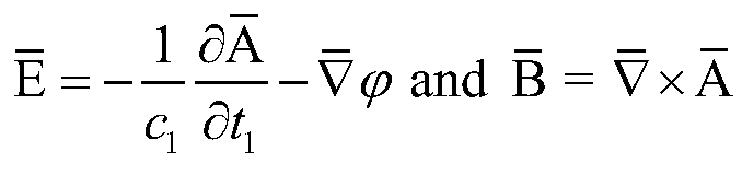
we get,
Appendix E
We can derive the well-known continuity equation for any value of h by examining Equation (6).
Applying · on both sides of the equation above,
References
- Zahir, S. Extra Time Dimension: Deriving Relativistic Space-Time Transformations, Kinematics, and Example of Dimensional Compactification Using Time-Dependent Non-Relativistic Quantum Mechanics. J. Mod. Phys. 2023, 14, 1333–1354. [Google Scholar]
- Velev, M. V. Relativistic mechanics in multiple time dimensions. Phys. Essays 2012, 25(3), 403–438. [Google Scholar] [CrossRef]
- “H. A. Lorentz, A. Einstein, H. Minkowski, and H. Weyl: The Principle of Relativity – a Collection of Original Memoirs”; Perrett, W.; Jeffery, G. B., Translators; Dover Publications, 1958. [Google Scholar]
- Sochichiu, C. Quantum Kaluza--Klein Compactification. Phys. Lett. 1999, B463, 27–32. [Google Scholar] [CrossRef]
- Rickles, D. A Brief History of String Theory; Springer-Verlag: Berlin, Heidelberg, 2014; ISBN 978-3-642-45127-0. [Google Scholar]
- Zahir, S. Effects of Compactification on Free Massive Scalar Fields in Five-Dimensional Space-Time with an Extra Time Dimension: Analysing Some Results. J. Mod. Phys. 2023, 14, 1600–1616. [Google Scholar]
- Tyagi, K.; Al-Shahristani, A. Behaviour of Particles in 2 Time Dimensional Spacetime with Separate Speeds of Causality through Dirac and Klein-Gordon Formulations. 2023. Available online: http://www.preprints.org. [CrossRef]
- Schröder, U. E. Special Relativity ISBN 981020132X. In World Scientific Lecture Notes in Physics; World Scientific Publishing Co. Pte. Ltd.: Singapore, 1990; Vol. 33. [Google Scholar]
- Jackson, J. D. Classical Electrodynamics, 2nd Edition; John Wiley & Sons, Inc.: New York, 1975; ISBN 0-471-43132-X. [Google Scholar]
- Field, J. H. A New Kinematical Derivation of the Lorentz Transformation and the Particle Description of Light. Helv. Phys. Acta 1997, 70(4), 542–564. [Google Scholar]
- Quigg, C. Gauge Theories of Strong, Weak, and Electromagnetic Interactions, 2nd Edition; Princeton University Press: Princeton, N.J., USA, 2013; ISBN 978-0-691-13548-9. [Google Scholar]
- Chaichian, M.; Nishijima, K. An Essay on Color Confinement, HIP-1999-60/TH. arXiv 1999, arXiv:hep. [Google Scholar]
- Wilson, K. G. Confinement of Quarks. Phys. Rev. D. 1974, 14, 2455. [Google Scholar]
- Greensite, J. The Confinement problem in lattice gauge theory, Prog. Part. Nucl. Phys. B 51, 1. arXiv [hep-lat]. 2003, arXiv:0301023. [Google Scholar]
- Mandelstam, S. Vortices and Quark Confinement in Nonabelian Gauge Theories. Phys. Rept. 1976, 23, 245–249. [Google Scholar] [CrossRef]
- ’t Hooft, Gerard. On the Phase Transition Towards Permanent Quark Confinement. Nucl. Phys. B 1978, 138, 1–25. [Google Scholar] [CrossRef]
- Kronfeld, Andreas S.; Laursen, M. L.; Schierholz, G.; Wiese, U. J. Monopole Condensation and Color Confinement. Phys. Lett. B 1987, 198, 516–520. [Google Scholar] [CrossRef]
- Nishijima, K. BRS Invariance, Asymptotic Freedom and Color Confinement (a Review) Czech. J. Phys. 1996, 46, 1–124. [Google Scholar] [CrossRef]
- Becchi, C.; Rouet, A.; Stora, R. Renormalization of Gauge Theories. Ann. Phys. 1976, 98, 287–321. [Google Scholar] [CrossRef]
- Gross, D. J.; Wilczek, F. Ultraviolet Behavior of Nonabelian Gauge Theories. Phys. Rev. Lett. 1973, 30, 1343–1346. [Google Scholar] [CrossRef]
- Politzer, H. D. Reliable Perturbative Results for Strong Interactions? Phys. Rev. Lett. 1973, 30, 1346–1349. [Google Scholar] [CrossRef]
- Deur, A.; Brodsky, S. J.; de Téramond, G. F. The QCD Running Coupling. Prog. Part. Nucl. Phys. 2016, 90, 1–74. [Google Scholar] [CrossRef]
- Anashin, V. V.; et al. Experiments with the KEDR Detector at the e+e− Collider VEPP-4M in the Energy Range √s = 1.84–3.88 GeV. Phys. Part. Nucl. 2023, 54(1), 185–226. [Google Scholar] [CrossRef]
- Ablikim, M.; et al. Measurement of the Cross Section for e + e − → Hadrons at Energies from 2.2324 to 3.6710 GeV. Phys. Rev. Lett. 2022, 128, 062004-1-9. [Google Scholar] [CrossRef] [PubMed]
- Weinberg, S. Gravitation and Cosmology; John Wiley & Sons: New York, 1972; ISBN 0-471-92567-5. [Google Scholar]
Short Biography of Authors
Dr. Sajjad Zahir is a Professor Emeritus, University of Lethbridge, Lethbridge, Alberta, Canada.
He completed graduate studies in both Theoretical Physics (Ph.D.) and Computer Science (M.S.) at the University of Oregon, Eugene, USA, and previously held research positions in Physics at several Canadian Universities. Then he worked in the areas of Decision Sciences/Management Sciences and Information Systems, first at Saint Mary’s University (1987-89) and then at the University of Lethbridge (UL) (1989-2016) as a Limited Term/Tenured Assistant, Associate, and Full Professor, and took an early retirement in 2016. He has published many research articles in physics, operations research, decision sciences, and information systems. He is still affiliated with the University of Lethbridge as Professor Emeritus and, in his own interest, active again in physics research. However, he is solely responsible for the content of his current physics research, and thus its results should have no bearing on the Physics Department at the University of Lethbridge, where he never worked. Dr. Zahir fully understands and respects the University of Lethbridge’s reputation and would be careful not to affect its image. For full information about Dr. Sajjad Zahir’s background, education, employment history, and research records, see his personal website https://sites.google.com/view/sajjadzahir/SajjadZahir.
Figure 1.
e+e- → quark + anti-quark plus gluon (source: https://handwiki.org/wiki/Physics:Gluon).
Figure 1.
e+e- → quark + anti-quark plus gluon (source: https://handwiki.org/wiki/Physics:Gluon).
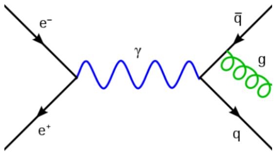

Table 1.
Calculation of Relevant Elements of the Field Tensor .
| 1) | |
| 2) | Similarly, the other relevant tensor elements are derived below. |
| 3) | |
| 4) | |
| 5) | |
| 6) | |
| 7) | |
| 8) | |
| 9) | |
| 10) |
Table 2.
Elements of the Field Tensor Fµν.
| 1) | |
| 2) | |
| 3) | |
| 4) | |
| 5) | |
| 6) | |
| 7) | |
| 8) | |
| 9) | |
| 10) |
Disclaimer/Publisher’s Note: The statements, opinions and data contained in all publications are solely those of the individual author(s) and contributor(s) and not of MDPI and/or the editor(s). MDPI and/or the editor(s) disclaim responsibility for any injury to people or property resulting from any ideas, methods, instructions or products referred to in the content. |
© 2026 by the author. Licensee MDPI, Basel, Switzerland. This article is an open access article distributed under the terms and conditions of the Creative Commons Attribution (CC BY) license.
Copyright: This open access article is published under a Creative Commons CC BY 4.0 license, which permit the free download, distribution, and reuse, provided that the author and preprint are cited in any reuse.


