Finite Memory and Infinite Transformation: A Clarification and Admissibility Scaffold for CIOU

1. Introduction

The word “infinite” is powerful, but it is also dangerous. In a physical theory it can sound like an escape from measurement, a metaphysical excess, or a claim that finite evidence can never discipline. The Infinite Transformation Principle, ITP, therefore requires a strict interpretation of its central word.

The same discipline is required for the word “organic” in CIOU. If left undefined, organic can sound like a claim that the universe is literally alive, conscious, or intentional. That is not the claim made here. The organic component is defined as the admissibility of nested, memory-bearing, disequilibrium-sustaining persistence systems inside a universe-level transformation architecture. Biological organisms are one local expression of such architecture, not the literal definition of the universe as an organism.

This article is a clarification and admissibility paper, not a complete physical theory of cyclic cosmology. Its purpose is to define what the terms “infinite”, “organic”, “cycle”, “inheritance”, and “ripeness” are allowed to mean inside the ITP/CIOU program once finite memory, finite saturation, and branch-specific falsification are imposed. A physical realization requires separate branch papers that supply concrete transfer operators, likelihoods, data mappings, and microphysical mechanisms.

The ITP parameter-space formalism has already made the local theory finite in the relevant technical sense. A physical realization belongs to a finite memory-bearing sector with irreversible structural growth before saturation, a causal memory kernel, finite structural capacity, and stabilizing long-wavelength response. In the minimal sector, the model is governed by seven parameters,

$$p=(\alpha ,m,S_{max},\Delta ,\beta ,\mu ,\eta )\in {\mathcal{M}}_{\mathrm{ITP}},$$

(1)

where $\alpha$, m, and $S_{max}$ describe structural production and saturation, $\Delta$ is the memory horizon, and $\beta$, $\mu$, and $\eta$ describe memory response and coupling [1]. The crucial point is simple: $S_{max}$ is finite and $\Delta$ is finite.

Therefore, the infinite in ITP cannot mean infinite memory. It cannot mean infinite structural storage. It cannot mean that a system carries its whole past as an undiminished archive. It cannot mean that a star, cell, galaxy, organism, or cosmic phase persists forever as itself.

The term has a narrower and more defensible meaning:

Infinite transformation means non-final continuation through finite, saturating, memory-bearing transformations.

The purpose of this article is to formalize that sentence without repeating the parameter-space derivation, the structural inheritance formalism, or the arrow-of-time argument. Those earlier papers already establish three ingredients. First, the ITP parameter paper defines the finite local model class. Second, the homeostatic-potential paper formalizes the structural inheritance code, previously called structural cosmic DNA, as compact internal code plus archived homeostatic memory [2]. Third, the arrow-of-time paper defines structural commitment as the irreversible reshaping of accessible configuration space [3]. This article asks what follows from those results for the permitted meaning of the vocabulary itself.

The answer is that infinity is not a local parameter. It is not an eighth coordinate of ${\mathcal{M}}_{\mathrm{ITP}}$. It is a boundary interpretation of how finite transformation sectors compose. Each sector is finite. The sequence of transformation is non-final only in the restricted sense that no finite form is granted absolute finality by definition.

This revision also addresses a presentation problem common to framework papers. A layered theory can begin to look self-referential if every paper presupposes every other one. The present paper therefore states its dependencies explicitly, introduces external theoretical anchors, labels synthetic tests as internal checks rather than physical evidence, and separates semantic clarification from physical realization.

2. Position in the Series and External Anchors

This article is part of a staged framework. It should not be read as the primary derivation of the ITP parameter space, the homeostatic-potential formalism, the structural-commitment arrow of time, or the Bayesian Memory Ladder evidence paper. Its role is narrower: to clarify the meaning of “infinite” after the local dynamics have already been restricted to finite memory and finite saturation.

3. Scope: Three Tiers of Claim

The claims in this article are divided into three tiers. This prevents a clarification paper from being mistaken for a completed cosmological theory.

The distinction is essential. A finite residue filter is not a quantum-gravity bounce mechanism. A synthetic cycle-filter test is not evidence that the universe cycles. A ripeness functional is not a universal law of maturation until a branch shows that it predicts something beyond late-history weighting. The present article defines the admissibility rules. It does not claim that all physical realizations have already been supplied.

The framework also sits near established literatures rather than outside them. Volterra integral equations formalize causal history dependence [27]. Mori-Zwanzig projection theory shows how memory kernels and noise terms arise when unresolved degrees of freedom are eliminated [21,29,30,31]. Nonlocal cosmology and nonlocal gravity show that history-dependent kernels can enter cosmological effective dynamics without being inserted as arbitrary metaphors [16,17,19,20,28]. The relevance of coarse-grained cosmological memory also places the present clarification near the backreaction problem in relativistic cosmology, where averaging inhomogeneous matter distributions can modify the effective large-scale evolution without introducing a new local matter component [14]. The TNG300 virialisation paper supplies the concrete simulation anchor for the coarse-grained memory-kernel example. The present paper does not identify CIOU with Buchert backreaction; it only notes that both frameworks treat large-scale cosmic evolution as sensitive to structure that is not captured by a strictly local homogeneous closure. Stochastic thermodynamics provides a separate language for irreversibility, dissipation, and finite-time fluctuations [15,18,25]. Causal-set approaches give another example where ordering and causal structure are treated as primitive or near-primitive physical data [13,26].

CIOU should also be distinguished from Penrose’s conformal cyclic cosmology, CCC [22,23,24]. Both frameworks reject a simple one-shot finality and both allow a kind of cycle-to-cycle inheritance. The difference is that the present article does not posit a conformal boundary, does not derive a Weyl-curvature hypothesis, and does not claim a CCC-like transmission mechanism. CIOU is used here only as a finite-sector renewal language: a cycle can transmit filtered structural residue only if a branch-specific transfer operator can be specified. The comparison is therefore a boundary marker, not an equivalence.

Classical nucleosynthesis and habitability literatures also matter for the organic component. The matter composing biological organisms is not external to cosmic history: heavy elements are produced through stellar and explosive nucleosynthetic processes [8,9]. Planetary habitability and photosynthetic energy capture then show how stellar output becomes a condition for long-lived biological chemistry rather than a distant background fact [10,11]. These facts do not prove that the universe is a literal organism. They justify treating biological systems as universe-internal expressions of cosmic material and energetic organization.

These references do not prove ITP. They define the technical neighborhood. The present article makes a narrower claim: if ITP uses the word “infinite”, it must do so without violating finite memory, saturation, causal kernels, or branch-level falsification.

4. What the Prior Formalism Already Fixes

The ITP parameter-space paper defines a restricted but useful class of systems. Such systems possess a scalar structural measure $S\left(t\right)$ and a memory functional $M\left(t\right)$. Their structural production is irreversible before saturation, their dynamics depend on a finite causal segment of their past, their structural capacity is bounded, and their long-wavelength memory response is contractive rather than explosive.

A minimal saturating structural law is

$$\dot{S}\left(t\right)=\alpha t^m\left(1-{\displaystyle \frac{S\left(t\right)}{S_{max}}}\right),\alpha >0,S_{max}>0,$$

(2)

with $m>-1$ in the simplest smooth time-weighted sector. The analytic solution for $S\left(0\right)=0$ is

$$S\left(t\right)=S_{max}\left[1-exp\left(-{\displaystyle \frac{\alpha }{(m+1)S_{max}}}{t}^{m+1}\right)\right].$$

(3)

The memory functional may be written as a causal Volterra object,

$$M\left(t\right)={\int }_0^{t}K(t-\tau )\Xi \left(\tau \right)d\tau ,$$

(4)

where $\Xi$ is a branch-specific structural source and K is causal and integrable. In the minimal single-timescale sector,

$$K\left(\tau \right)={\displaystyle \frac{1}{\Delta }}exp\left(-{\displaystyle \frac{\tau }{\Delta }}\right)\Theta \left(\tau \right),$$

(5)

where $\Delta >0$ is the characteristic memory horizon. The equivalent local auxiliary form is

$$\dot{M}\left(t\right)+{\displaystyle \frac{1}{\Delta }}M\left(t\right)=\Xi \left(t\right),$$

(6)

and for the parameter-space scaffold $\Xi \left(t\right)=\dot{S}\left(t\right)$.

This means that the local ITP sector is not a theory of limitless memory. It is explicitly a theory of finite memory. It is also not a theory of limitless structural growth. It is explicitly a theory of saturation,

$$\underset{t\to \infty }{lim}S\left(t\right)=S_{max}<\infty .$$

(7)

The seven-parameter manifold can be written as

$${\mathcal{M}}_{\mathrm{ITP}}=\left\{(\alpha ,m,S_{max},\Delta ,\beta ,\mu ,\eta ):\alpha >0,S_{max}>0,\Delta >0,\mu \ge 0,(\beta ,\eta )\in {\mathbb{R}}^2\right\}.$$

(8)

The new article therefore begins from a constraint:

$$\mathrm{infinite}\mathrm{transformation}\ne \Delta \to \infty ,$$

(9)

$$\mathrm{infinite}\mathrm{transformation}\ne S_{max}\to \infty .$$

(10)

Taking either limit would not clarify ITP. It would damage it. If $\Delta \to \infty$, the finite-memory axiom collapses. If $S_{max}\to \infty$, the saturation axiom collapses. The word “infinite” must therefore be located somewhere else.

5. What Infinite Cannot Mean

The first task is negative. The word must be protected from weak interpretations.

First, infinite transformation does not mean infinite storage. A system does not retain all past states. It retains selected consequences of past states through finite variables, kernels, residues, and constraints. Equation (4) already makes this clear. Memory is causal, weighted, and integrable. It is not a complete database of the past.

Second, infinite transformation does not mean immortality of form. A star can die, a cell can die, an organism can die, a galaxy can merge, a local homeostatic basin can collapse, and a cosmic phase can end. These endings are real at the level of identity. The principle does not deny them.

Third, infinite transformation does not mean exact recurrence. A cycle is not a replay. A universe that cycles need not return to the same state, with the same contents and the same sequence of events. Exact recurrence is too rigid for a non-Markovian framework, because memory and commitment alter the conditions under which the next phase begins.

Fourth, infinite transformation does not mean that infinity is directly measured as an empirical object. No finite observer measures an infinite sequence. What can be tested are finite projections of the principle: memory kernels, structural persistence, path dependence, code gain, basin occupancy, recoverability, commitment, and model comparison against Markovian baselines.

The positive claim is therefore more modest and more useful:

No finite state is granted absolute finality by the framework.

This is not a claim that every object continues forever. It is a claim that the end of an object is not identical to the end of transformation.

6. Finite Sectors and Non-Final Composition

Let $X_n$ denote the state of a system or phase at a finite transformation index n. Let

$$p_n=({\alpha }_n,m_n,S_{max,n},{\Delta }_n,{\beta }_n,{\mu }_n,{\eta }_n)$$

(11)

be its local ITP parameter vector, with

$$0<S_{max,n}<\infty ,0<{\Delta }_n<\infty .$$

(12)

Let $g_n$ denote the inherited structural constraint map, and let $C_n$ denote accumulated structural commitment. A finite transformation sector is then represented by the tuple

$${\mathcal{S}}_n=(X_n,p_n,g_n,C_n).$$

(13)

A transformation step is written schematically as

$${\mathcal{S}}_{n+1}={\mathcal{T}}_n({\mathcal{S}}_n,{\epsilon }_n),$$

(14)

where ${\epsilon }_n$ denotes perturbation, novelty, environmental forcing, or unresolved degrees of freedom.

Equation (14) does not say that the same identity persists. It says that one finite sector can pass residue, structure, constraint, or transformed material into another finite sector. This distinction is central. A form-level terminal event may occur when the form can no longer maintain its own basin. But that does not imply an absolute transformation-level terminal event.

Let ${\mathcal{A}}_{\mathrm{form}}\left({\mathcal{S}}_n\right)$ be the admissible continuation set for the same form, and let ${\mathcal{A}}_{\mathrm{trans}}\left({\mathcal{S}}_n\right)$ be the admissible transformation set for the residual structure, material, energy, or constraint left by that form. Then a local death, collapse, or dissolution may be expressed as

$${\mathcal{A}}_{\mathrm{form}}\left({\mathcal{S}}_n\right)=⌀,$$

(15)

while non-final transformation requires only

$${\mathcal{A}}_{\mathrm{trans}}\left({\mathcal{S}}_n\right)\ne ⌀.$$

(16)

Definition 1 

(Non-final transformability). A finite transformation sector is non-final if its form may terminate while its residual structure, material, energetic content, or constraint can enter at least one further admissible transformation sector.

Definition 2 

(Infinite transformation). The Infinite Transformation Principle interprets infinity as indefinite finite-sector composition: for any finite N, there exists an admissible sequence

$${\mathcal{S}}_0\to {\mathcal{S}}_1\to \dots \to {\mathcal{S}}_N,$$

(17)

where each local sector has finite memory and finite saturation capacity. The principle does not require any single form, identity, or memory archive to persist through all sectors.

This definition preserves the provocative force of the word while keeping the physics finite. Each step is finite. The composition is non-final.

7. The Structural Inheritance Code

If memory is finite, a second problem appears. Why is transformation not random? If the system does not remember everything, and if no state is final, what carries continuity?

This is where the structural inheritance code enters. The phrase “structural cosmic DNA” remains useful as a metaphor, but it is technically risky if it sounds biological or literal. In this article the technical object is therefore the finite structural inheritance code $g_n$. The phrase “structural cosmic DNA” is retained only as a heuristic name for this code. No biological literalism is implied, and no claim is made that the universe contains a DNA-like substance.

The homeostatic-potential formalism defines a structural code through visible dynamics of the form

$$\dot{x}\left(t\right)=F_{\theta }\left(x\left(t\right),e\left(t\right),m_{\varphi }\left(t\right)\right),$$

(18)

where $x\left(t\right)$ is the observable state, $e\left(t\right)$ is the environment, $\theta$ are compact internal structural parameters, and $m_{\varphi }\left(t\right)$ is archived homeostatic memory. The archived memory is not neutral storage. It is homeostatic relevance filtered through a causal kernel,

$$m_{\varphi }\left(t\right)={\int }_0^t{K}_{\theta }(t-\tau )Q_{\varphi }\left(\widehat{\varphi }\left(\tau \right)\right)\Psi \left(x\left(\tau \right),e\left(\tau \right)\right)d\tau .$$

(19)

Here $Q_{\varphi }$ is the relevance weighting and $\Psi$ is the branch-specific source being archived.

In the present article, the full derivation of the homeostatic potential is not repeated. It is compressed into the following object:

$$g_n=\mathcal{G}\left({\theta }_n,m_{\varphi ,n},p_n\right),$$

(20)

where $g_n$ is a finite constraint map carried by sector n.

Definition 3 

(Structural inheritance code as a finite constraint map). Let $X_n$ denote the state of a finite transformation sector, let $p_n\in {\mathcal{M}}_{\mathrm{ITP}}$ denote its finite ITP parameter location, and let $C_n$ denote accumulated structural commitment. A structural inheritance code is a compact, finite, non-Markovian constraint map

$$g_n=\mathcal{G}(X_n,p_n,C_n,m_n),$$

where $m_n$ is the finite memory state available to sector n. The object $g_n$ does not denote linguistic syntax, biological DNA, intentional design, or a complete historical archive. It denotes the finite constraint structure by which prior transformations modify the admissible transformations of the next sector.

In this usage, the word “code” is technical shorthand for a constraint-bearing state descriptor. A branch model earns this language only when $g_n$ improves the description of future states beyond an environment-only or Markovian closure. If $g_n$ cannot be operationally estimated, cannot be distinguished from ordinary causal history, or does not improve prediction under appropriate null tests, then the structural-inheritance interpretation fails in that branch.

8. Structural Commitment as the Direction of Continuation

Transformation is not only change. If every change could be freely undone, transformation would have sequence but no deep arrow. The arrow appears when transformation commits the future.

The arrow-of-time formalism defines structural commitment as the irreversible reshaping of accessible configuration space. Let ${\Omega }_0$ denote an initial possibility space, and let $C\left(t\right)$ denote cumulative structural commitment. The effective possibility space is

$${\Omega }_{\mathrm{eff}}\left(t\right)={\Omega }_0\setminus C\left(t\right).$$

(21)

This equation does not require that possibility space only shrinks in a crude numerical sense. Some commitments may open new structured possibilities while closing prior freedoms. The key is that the geometry of accessibility has changed. The future is not the same future after the commitment.

In discrete form,

$$C_{n+1}=C_n\cup \Delta C_n,$$

(22)

with

$${\Omega }_{n+1}=\mathcal{K}({\Omega }_n,C_{n+1}),$$

(23)

where $\mathcal{K}$ is a branch-specific commitment operator.

The homeostatic-potential formalism gives a related local measure. If ${\Omega }_{\varphi }\left(t\right)$ is the accessible homeostatic state space, then structural commitment may be measured as

$${\Gamma }_{\varphi }\left(t\right)=-{\displaystyle \frac{d}{dt}}ln\left|{\Omega }_{\varphi }\left(t\right)\right|.$$

(24)

Positive ${\Gamma }_{\varphi }$ indicates shrinking viable breadth, negative ${\Gamma }_{\varphi }$ indicates reopening or expansion of viable breadth, and near-zero ${\Gamma }_{\varphi }$ indicates maintained breadth.

This makes the arrow of time different from mere chronology. Chronology says

$$t\to t+\Delta t.$$

(25)

Structural commitment says

$${\Omega }_t\to {\Omega }_{t+\Delta t},{\Omega }_{t+\Delta t}\ne {\Omega }_t$$

(26)

under irreversible transformation. The past is not physically consequential because it is perfectly remembered. It is consequential because it has changed what the future can be.

The relationship among the core terms can now be stated cleanly:

$$\begin{array}{|c|}\hline \begin{array}{c}\mathrm{finite}\mathrm{memory}\to \mathrm{structural}\mathrm{inheritance}\mathrm{code}\to \mathrm{structural}\mathrm{commitment}\\ \to \mathrm{directed}\mathrm{non}-\mathrm{final}\mathrm{transformation}\end{array}\\ \hline\end{array}$$

(27)

Memory says what remains. The structural inheritance code says how what remains can generate. Structural commitment says what can no longer be undone. Infinite transformation says no finite state is absolute finality.

9. CIOU as Cyclic Renewal, Not Exact Repetition

The Cyclical Infinite Organic Universe, CIOU, uses the same logic at cosmological scale. Here the word “cyclical” must also be protected from a weak interpretation. Cyclical does not mean exact repetition. A cycle is not a rewind.

This paper uses a deliberately minimal definition of a cycle. A cycle is a finite transformation sector with its own state trajectory, ITP parameter location, memory horizon, saturation capacity, inherited constraint map, and accumulated commitment. This article does not derive the microphysics of a cosmic phase transition. It defines the inheritance structure required for a cycle-to-cycle claim to be meaningful.

Let $X_k$ denote a cosmic phase, $p_k$ its finite ITP sector, $g_k$ its inherited structural constraint map, and $C_k$ its accumulated commitment. A CIOU transition may be written as

$$X_{k+1}={\mathcal{C}}_{\mathrm{cyc}}(X_k,p_k,g_k,C_k,{ϵ}_k),$$

(28)

where ${ϵ}_k$ represents novelty, perturbation, stochastic residue, or unresolved transition structure.

The framework does not require

$$X_{k+1}=X_k.$$

(29)

In general,

$$X_{k+1}\neg \equiv X_k.$$

(30)

A cycle-to-cycle claim is admissible only if it specifies: the pre-transition state variables, the finite residue operator, the projection back into the allowed ITP parameter manifold, the null models of random reset and exact recurrence, and at least one observable carried into the next sector.

This is the crucial distinction. CIOU is not a universe that exactly replays the same sequence. It is a universe in which phases renew through finite inherited structure. Each phase may carry enough memory to constrain the next phase, but not enough to reproduce the entire past exactly.

The compact statement is:

CIOU is cyclical without exact repetition, infinite without infinite memory, and organic without biological literalism.

The term “organic” also requires discipline. It does not mean that the universe is literally biological. It means that the universe is treated as a nested, regulated, memory-bearing transformation system. Its parts interact across scale. Its structures inherit constraints. Its futures are shaped by accumulated commitments. Its local forms arise, persist, decay, dissolve, and re-enter transformation.

Thus, the organic claim is structural rather than biological.

10. Organic Admissibility in CIOU

The compact phrase “organic without biological literalism” needs a formal definition. Otherwise the word organic becomes vulnerable to two opposite errors. The first error is biological inflation: treating the universe as if it were literally an animal, plant, cell, mind, or intentional organism. The second error is sterile reduction: treating life as though it were outside the universe and therefore irrelevant to the universe’s own transformation architecture.

CIOU avoids both errors. The claim is not that the universe is biologically alive. The claim is that the universe is capable of generating nested, memory-bearing, disequilibrium-sustaining persistence systems, of which biological organisms are one local realized expression. This is a structural admissibility claim, not a zoological claim.

There are three levels of organicity. The weakest is compositional organicity: living organisms are made of matter produced through cosmic processes and are sustained by cosmic energy gradients. This is true but insufficient. The fact that a system contains life does not by itself make the whole system an organism. The second is generative organicity: the universe supplies the material, stellar, planetary, chemical, and atmospheric pathways through which life-compatible systems can arise. The third, and the only one used technically here, is structural organicity: a universe phase is organic-admissible when it can generate localized systems that retain matter, buffer forcing, sustain bounded disequilibrium, preserve structural memory, and support recursive complexity.

Let $U_k$ denote a cosmic phase or cycle, and let $x\subset U_k$ denote a localized subsystem. Let

$$q\left(x\right)=\left(C_{\mathrm{mat}},G_{\mathrm{flux}},P_{\mathrm{pers}},D_{\mathrm{diseq}},R_{\mathrm{rec}},M_{\mathrm{struct}}\right)$$

(31)

denote normalized material, energetic, persistence, disequilibrium, recursive-complexity, and memory terms. Organic admissibility is not a single law at this stage. It is an admissibility family. Three simple branch-level choices are permitted:

$${\mathcal{O}}_{\mathrm{add}}\left(x\right)=\sum _i{w}_i{q}_i\left(x\right),$$

(32)

$${\mathcal{O}}_{\mathrm{mult}}\left(x\right)=\prod _i{q}_i{\left(x\right)}^{w_i},$$

(33)

$${\mathcal{O}}_{\mathrm{gate}}\left(x\right)=\prod _i\mathbf{1}\left[q_i\left(x\right)>q_{i,★}\right].$$

(34)

The additive form allows tradeoffs among terms. The multiplicative form penalizes the collapse of any required component. The gate form is the strictest threshold version. A branch paper must specify which form is used, how the weights or thresholds are estimated, and what null model would falsify the chosen construction.

A cosmic phase is organically admissible when

$$U_k\mathrm{is}\mathrm{organically}\mathrm{admissible}⟺\exists x\subset U_k\mathrm{such}\mathrm{that}\mathcal{O}\left(x\right)>{\mathcal{O}}_{★},$$

(35)

where $\mathcal{O}$ is one declared member of the admissibility family. The threshold ${\mathcal{O}}_{★}$ must be estimated from branch-specific reference populations, quantiles, posterior credible regions, physically motivated corridors, or pre-registered stability conditions. It must not be chosen after interpretation has hardened. This definition does not claim life detection. It defines the conditions under which life-compatible or recursive-complexity-bearing structures can be generated and sustained.

The layered exoplanet persistence framework gives a local example of this logic. It does not claim biosignature detection, intelligence, consciousness, or inhabited systems. Instead, it builds adaptive, occupancy, atmospheric, uncertainty, and chemical-proxy layers and asks whether persistence morphologies survive coherence constraints and uncertainty propagation [7]. In that language, coherent persistence basins, adaptive-shadow systems, latent persistence candidates, and adaptive instability frontiers are not declarations of life. They are local tests of whether layered persistence morphology can be made operational under bounded proxies.

The abundance or measure of organic admissibility in a phase may be written schematically as

$${\mathcal{O}}_{\mathrm{CIOU}}\left(U_k\right)={\int }_{{\Omega }_k}\mathbf{1}\left[\mathcal{O}\left(x\right)>{\mathcal{O}}_{★}\right]d{\mu }_k\left(x\right),$$

(36)

where ${\Omega }_k$ is the accessible state space of phase k and ${\mu }_k$ is the relevant measure on localized subsystems. This quantity may be zero in a sterile phase, small in a marginal phase, or large in a phase rich in persistence-bearing structures. CIOU does not require life everywhere. It requires only that organic admissibility can be generated, filtered, lost, or renewed through finite transformation.

In a cyclic setting, organicity is not the passage of organisms from one cycle to the next. It is the finite inheritance of organic admissibility conditions. A cycle-to-cycle organic residue can be written as

$$r_k^{\mathrm{org}}={\displaystyle \frac{{\int }_0^{T_k}{W}_{\mathrm{org}}\left(t\right)z_k\left(t\right)dt}{{\int }_0^{T_k}{W}_{\mathrm{org}}\left(t\right)dt}},$$

(37)

where $z_k\left(t\right)$ is the structural state of cycle k, and $W_{\mathrm{org}}\left(t\right)$ weights matter retention, energy-gradient stability, bounded disequilibrium, layered persistence geometry, and structural memory. The next phase receives a filtered admissibility residue,

$${\mathcal{O}}_{k+1}={\mathcal{R}}_{\mathrm{org}}\left(r_k^{\mathrm{org}},g_k,C_k,{ϵ}_k\right),$$

(38)

rather than a complete biological archive.

Definition 4 

(Organic admissibility). A universe phase is organically admissible when its physical structure permits localized subsystems to retain matter, process energy gradients, sustain bounded disequilibrium, preserve structural memory, and support recursive complexity under a declared admissibility functional. Organic admissibility is a condition on regenerative persistence, not a claim of cosmic consciousness, intention, or literal biological organismhood.

This definition can fail. It fails if organicity reduces only to the fact that life exists somewhere, because that is too weak to distinguish CIOU from ordinary cosmology. It fails if organicity is used to smuggle in intention, consciousness, or literal organismic unity. It fails empirically if layered persistence morphologies disappear under expanded samples, if chemical-proxy layers fail against independent atmospheric retrievals, if thresholds cannot be pre-specified, or if cycle-to-cycle organic residues perform no better than random reset. The measure $d{\mu }_k\left(x\right)$ must be specified by the branch using the organic-admissibility functional. It is not a universal measure over all conceivable subsystems. In a cosmological branch, admissible choices may include a comoving-volume measure, a halo-mass-function weighting, a stellar-mass weighting, a baryonic-mass weighting, or a planet-occurrence weighting, depending on the class of localized systems being tested. In an exoplanet branch, $d{\mu }_k\left(x\right)$ may be replaced by a catalog-weighted or completeness-weighted sum over observed systems. Thus,

$${\mathcal{O}}_{\mathrm{CIOU}}\left(U_k\right)={\int }_{{\Omega }_k}\mathbf{1}\left[\mathcal{O}\left(x\right)>{\mathcal{O}}_{★}\right]d{\mu }_k\left(x\right)$$

is not an assertion that organic-admissible structure exists everywhere. It is a weighted abundance or occupancy measure over a declared subsystem ensemble.

A corresponding null model must also be stated. Let $U_k^{\left(0\right)}$ denote a null universe or null ensemble in which the same matter budget, survey selection, and marginal distributions are preserved, but the coupling among material continuity, energy-gradient throughput, persistence, disequilibrium, recursive complexity, and memory is destroyed by shuffling, phase randomization, environment-only closure, or another branch-appropriate null operation. Organic admissibility is supported only if

$${\mathcal{O}}_{\mathrm{CIOU}}\left(U_k\right)>{\mathbb{E}}_0\left[{\mathcal{O}}_{\mathrm{CIOU}}\left(U_k^{\left(0\right)}\right)\right]+{\lambda }_{\mathrm{null}}{sd}_0\left[{\mathcal{O}}_{\mathrm{CIOU}}\left(U_k^{\left(0\right)}\right)\right],$$

for a predeclared threshold ${\lambda }_{\mathrm{null}}$, or if the corresponding posterior probability exceeds a branch-specified evidential threshold. If the observed value is indistinguishable from the null ensemble, the organic-admissibility claim fails for that branch.

For the gate functional, this condition is especially important. A single localized subsystem satisfying $\mathcal{O}\left(x\right)>{\mathcal{O}}_{★}$ is not sufficient unless the measure, threshold, selection function, and null ensemble have been fixed before interpretation. Otherwise the claim becomes trivially satisfiable: almost any large universe could contain at least one apparently admissible subsystem by chance.

11. Ripeness as Non-Teleological Homeostatic Maturation

The organic component also requires a maturation concept. Not every system that persists is mature, and not every saturated system is homeostatically balanced. Ripeness is introduced here as a candidate homeostatic-maturation weighting that distinguishes mere persistence from balanced viability. It is not yet a validated universal variable.

Ripeness does not imply purpose, intention, consciousness, or biological desire. A system does not aim at homeostasis in a psychological sense. Rather, systems that enter viable homeostatic basins tend to persist longer, resist perturbation more effectively, and contribute more coherent residue to later transformations. Ripeness is therefore a viability-filtered dynamical condition, not a teleological claim.

Let

$$\varphi \left(t\right)=\left(H\right(t),R(t),S(t),M(t\left)\right)$$

(39)

be the HRSM state vector, and let ${\mathcal{A}}_{\varphi }$ denote a viable HRSM basin. Define distance from homeostatic viability as

$$D_{\varphi }\left(t\right)=d\left(\varphi \left(t\right),{\mathcal{A}}_{\varphi }\right).$$

(40)

Let $\Xi \left(t\right)$ denote environmental dominance, where $\Xi \left(t\right)<1$ indicates that internal structural code dominates environmental pressure. Let ${\Gamma }_{\varphi }\left(t\right)$ be structural commitment as in Eq. (24).

A system is ripening when it is moving toward the viable basin:

$${\displaystyle \frac{d{D}_{\varphi }}{dt}}<0,{\displaystyle \frac{d\Xi }{dt}}<0,R\left(t\right)>R_{★}.$$

(41)

A system is ripe when it has achieved maintained homeostatic maturity:

$$D_{\varphi }\left(t\right)\le ϵ,\Xi \left(t\right)<1,\left|{\Gamma }_{\varphi }\left(t\right)\right|\le {\gamma }_{★},$$

(42)

with recoverability $R\left(t\right)$ above threshold and memory $M\left(t\right)$ remaining inside an admissible bounded range.

Structural commitment and ripeness are not the same quantity. Commitment is the directional accumulation of constraint. Ripeness is a regime condition inside that committed space. A ripening system may have ${\Gamma }_{\varphi }<0$ during recovery or ${\Gamma }_{\varphi }>0$ during stabilization. A ripe system is not commitment-free; rather, it has reached a regime in which commitment no longer rapidly narrows viable futures. Ripeness therefore corresponds to bounded or regulated commitment, not absence of commitment.

Ripeness is also not equivalent to saturation. Saturation describes finite structural capacity. Ripeness describes balanced viability inside that capacity. A system may be saturated yet pathological if it retains memory without recoverability, or if structural commitment narrows its future state space too strongly. Cancer-like regimes, for example, may exhibit persistence without healthy recoverability. Such systems are not ripe; they are cases of distorted survival.

For observed or partially observed systems, ripeness must be measurement-aware. Let

$$P_{\varphi }\left(t\right)={\varphi }_{\mathrm{metric}}\left(t\right)P_{\mathrm{occ},\varphi }\left(t\right)C_{\mathrm{complete},\varphi }\left(t\right)C_{\mathrm{spread},\varphi }\left(t\right)$$

(43)

denote the observable homeostatic persistence score. This mirrors the layered persistence logic used in exoplanet screening, where occupancy probability, completeness, and spread coherence are kept separate from primitive structural metrics [7]. A candidate ripeness functional may then be written schematically as

$${\mathcal{R}}_{\varphi }\left(t\right)=P_{\varphi }\left(t\right)C_{\mathrm{mat}}\left(t\right)C_{\Xi }\left(t\right)C_{\Gamma }\left(t\right)C_R\left(t\right)C_M\left(t\right),$$

(44)

where $C_{\mathrm{mat}}$ measures structural maturation, $C_{\Xi }$ penalizes environmental domination, $C_{\Gamma }$ penalizes excessive narrowing of future possibility space, $C_R$ enforces recoverability, and $C_M$ enforces bounded memory rather than unbounded burden. These factors are not unique. A branch paper must justify their forms, report sensitivity, and show that the ripeness functional contributes something beyond a generic late-history or persistence filter. The exoplanet persistence application should therefore be read as a local demonstration of how an organic-admissibility measure might be implemented under partial observability, not as validation of CIOU. Its layered persistence quantities are catalog-dependent, proxy-level, and explicitly not biosignature detections. In the notation above, the exoplanet case replaces the abstract measure $d{\mu }_k\left(x\right)$ with a completeness-aware finite catalog sum and tests whether persistence morphologies remain stable under uncertainty propagation, latent-mass recovery, atmospheric-proxy extension, and chemical-proxy extension. In a cyclic setting, ripeness can modify the inheritance operator. The next cycle does not inherit the whole previous history. It inherits a finite, relevance-weighted residue. If ripeness is included, the residue becomes

$$r_k^{\mathrm{ripe}}={\displaystyle \frac{{\int }_0^{T_k}{K}_f(T_k-t){\mathcal{R}}_{\varphi ,k}\left(t\right)z_k\left(t\right)dt}{{\int }_0^{T_k}{K}_f(T_k-t){\mathcal{R}}_{\varphi ,k}\left(t\right)dt}},$$

(45)

where $z_k\left(t\right)$ is the structural state of cycle k, $K_f$ is the finite memory filter, and ${\mathcal{R}}_{\varphi ,k}$ weights the portions of the cycle that achieved homeostatic maturity. The next finite ITP sector may then be written as

$$p_{k+1}={\Pi }_{{\mathcal{M}}_{\mathrm{ITP}}}\left[A_0+A_1{r}_k^{\mathrm{ripe}}+{ϵ}_k\right].$$

(46)

Thus cycle-to-cycle inheritance is not total historical transfer. It is, at most, ripeness-weighted residue transfer where a branch validates ripeness as technically useful.

Definition 5 

(Candidate ripeness functional). Ripeness is a candidate non-teleological homeostatic-maturation weighting for systems whose HRSM state remains close to a viable basin, whose internal code buffers environmental forcing, whose recoverability has not collapsed, and whose memory remains bounded rather than burdensome. In this paper ripeness is classificatory, not yet a validated universal variable.

This concept can fail. It fails if ripeness collapses into age, saturation, or simple persistence. It fails if high memory is treated as mature even when recoverability is lost. It fails if the ripeness-weighted residue does not predict next-sector structure better than shuffled, random-reset, or generic late-filter residues. It also fails if the claimed homeostatic basin disappears under uncertainty propagation, expanded samples, or alternate proxy definitions. The synthetic scaffold in Sec. Section 13 shows that ripeness can be implemented, but because it performs nearly like a generic late structural filter in the toy data, it has not yet earned independent predictive status.

12. Empirical Meaning and Falsification

The infinite part of the theory is not directly measured. No finite observation proves an infinite sequence. The empirical content lies in finite projections of the principle. These projections include finite memory kernels, non-Markovian predictive gain, structural-code gain, basin persistence, recoverability, commitment, and model comparison against Markovian or environment-only baselines.

12.1. Code Gain

The homeostatic-potential formalism gives a direct predictive falsifier. Define

$$I_{\mathrm{code}}=H(X_{t+\Delta t}\mid X_t,E_t)-H(X_{t+\Delta t}\mid X_t,E_t,\theta ,m_{\varphi }).$$

(47)

Here $H(·)$ denotes conditional entropy. If

$$I_{\mathrm{code}}>0,$$

(48)

then the structural code reduces predictive uncertainty. If

$$I_{\mathrm{code}}\le 0,$$

(49)

then the structural-code hypothesis fails for that branch.

This is a useful discipline. The structural inheritance code is not accepted because the phrase is powerful. It must improve prediction or preserve interpretable structure under perturbation. Classical entropy arguments beginning with Boltzmann motivate the thermodynamic side of irreversibility, while stochastic thermodynamics supplies modern fluctuation relations and finite-time dissipation constraints [12,15,18,25].

12.2. Bayesian Evidence as a Falsification Gate

Bayesian evidence is not the foundation of this article. The BML evidence belongs in its own evidence paper. Here it enters only as a falsification gate for one finite-memory cosmological realization. The Bayesian Memory Ladder evidence paper is therefore treated as a separate branch-level evidence report rather than as the foundation of the present clarification [4].

Let $Z_{\mathrm{mem}}$ be the evidence for a restricted memory model and $Z_{\mathrm{base}}$ the evidence for its matched Markovian or $\Lambda$CDM baseline. Define

$$\Delta logZ=log{Z}_{\mathrm{mem}}-log{Z}_{\mathrm{base}}.$$

(50)

In a BML branch, the memory model may be parameterized by restricted kernel or window quantities such as

$$(\gamma ,T_0,{\sigma }_T),$$

(51)

or by reduced ITP-like quantities such as

$$(ϵ,\Delta ),$$

(52)

where $ϵ$ is a memory amplitude and $\Delta$ is the characteristic memory horizon.

Criterion 1 

(Cosmological memory evidence gate). A restricted cosmological memory branch fails its evidence test if

$$\Delta logZ\le 0$$

(53)

consistently under matched likelihoods, matched priors, converged sampling, stable numerical settings, and posterior predictive checks.

This criterion does not falsify infinity directly. It falsifies one proposed finite-memory realization of the transformation framework. That distinction matters. The article is not claiming that Bayesian evidence proves infinite transformation. It is saying that finite memory branches must earn their complexity penalty where they are claimed to operate.

12.3. Branch-Level Failure Conditions

The framework should be allowed to fail.A framework that cannot fail is not scientifically constrained.

The shortest version is:

The framework fails wherever finite memory has no structural consequence.

13. Minimal Robustness Scaffolds

The previous equations can still be criticized as formal decoration unless they generate checks that can pass or fail. This section therefore adds a small numerical robustness scaffold. The tests are deliberately minimal. They are synthetic internal-consistency and null-separation checks. They do not establish physical cyclic cosmology, do not test prior-cycle fossils, and do not claim empirical validation. Their purpose is to verify that the finite equations used above are operational, that local implementations reproduce convolution definitions, and that the proposed language of cycle-to-cycle inheritance can be represented by a finite residue operator with explicit null models.

All tests in this section were run with the scripts supplied alongside this draft:

scripts/01verifysaturatinggrowth.py, scripts/02cyclefiltermapping.py, scripts/04cyclesensitivityandripeness.py, scripts/03runall.py.

The generated tables are stored under results/tables/, and the figures under results/figures/. The scripts use synthetic data and fixed random seeds. In the cycle-filter experiments, the data-generating process includes finite residue structure, so recovery of that structure demonstrates implementability and null separation rather than independent prediction.

13.1. Test 1: Saturating Structural Growth

The first test verifies Eq. (2) against its analytic solution in Eq. (3). The sweep varies $\alpha$, m, and $S_{max}$ across six parameter settings. The script checks numerical solution error, monotonicity violations, final saturation error, and time to reach 95 and 99 percent of $S_{max}$.

Across the six settings, the run produced zero monotonicity violations. The maximum numerical-versus-analytic error was below $4.45\times {10}^{-5}$, with most settings below $2\times {10}^{-6}$. The synthetic noisy parameter recovery used true values

$$(\alpha ,m,S_{max})=(0.75,0.25,1.00)$$

(54)

and recovered

$$(\widehat{\alpha },\widehat{m},{\widehat{S}}_{max})\simeq (0.745,0.248,0.9998),$$

(55)

with RMSE $\simeq 1.47\times {10}^{-2}$ for noise level $\sigma =0.015$.

This test answers one narrow concern. The growth equation is not merely written down. It can be solved, checked against its analytic solution, fitted back from synthetic data, and made to fail if it violates monotonicity or saturation.

13.2. Test 2: Auxiliary Memory Versus Convolution Memory

The second test validates the local auxiliary representation against the direct convolution. For the exponential kernel, the memory functional can be computed either by direct quadrature,

$$M_{\mathrm{conv}}\left(t\right)={\int }_0^t{\displaystyle \frac{1}{\Delta }}exp\left[-{\displaystyle \frac{t-\tau }{\Delta }}\right]\dot{S}\left(\tau \right)d\tau ,$$

(56)

or by the auxiliary ODE,

$$\dot{M}\left(t\right)+{\displaystyle \frac{1}{\Delta }}M\left(t\right)=\dot{S}\left(t\right),M\left(0\right)=0.$$

(57)

The simulation used $\Delta =1.25$. The maximum absolute difference between the two implementations was $1.80\times {10}^{-4}$, and the RMSE was $9.40\times {10}^{-6}$.

This is a necessary implementation check. If the auxiliary equation failed to reproduce the convolution, the finite-memory scaffold would fail before any physical interpretation began.

13.3. Test 3: Finite Cycle-Filter Inheritance

The cycle-filter test addresses the weakest part of any cyclic inheritance claim: how is one cycle filtered into the next? The test does not assume that a whole previous cycle is copied. It defines a finite late-cycle residue,

$$r_k={\displaystyle \frac{{\int }_0^{T_k}exp[-(T_k-t)/{\Delta }_f]Q\left(S_k\left(t\right)\right)z_k\left(t\right)dt}{{\int }_0^{T_k}exp[-(T_k-t)/{\Delta }_f]Q\left(S_k\left(t\right)\right)dt}},$$

(58)

where $z_k\left(t\right)$ contains the cycle state, memory state, growth rate, and commitment proxy, and $Q\left(S_k\right)$ is a relevance weighting. The next cycle’s reduced parameter vector is generated by

$$p_{k+1}={\Pi }_{{\mathcal{M}}_{\mathrm{ITP}}}\left[A_0+A_1{r}_k+{\xi }_k\right],$$

(59)

where $p_k=({\alpha }_k,m_k,S_{max,k},{\Delta }_k)$ in this minimal simulation, ${\xi }_k$ is noise, and ${\Pi }_{{\mathcal{M}}_{\mathrm{ITP}}}$ projects the generated parameters back into the allowed ITP sector. The synthetic data were generated by this finite-residue architecture. Therefore, the high $R^2$ values below should not be read as physical predictability of cosmic cycles. They show that the proposed operator can be implemented, recovered, and distinguished from shuffled-cycle and mean-only nulls under controlled conditions.

This is the computational form of the statement:

A cycle does not transmit its whole history. It transmits a finite, relevance-weighted residue that modifies the next sector’s admissible parameter location.

The same run reports that near-identical cycle repetition is rare under a 1 percent scale criterion: approximately 0.37 percent for $\alpha$, 0.74 percent for m, 0.74 percent for $S_{max}$, and 1.48 percent for $\Delta$. Thus the synthetic cycle model is not exact recurrence. It is renewal with finite inherited constraint.

The null tests matter more than the positive scores, and the absolute $R^2$ values should not be interpreted as empirical performance. If shuffled cycle histories predicted $p_{k+1}$ as well as the finite residue, cycle inheritance would fail. If exact recurrence matched the data, the framework would collapse into repetition. If the entire previous trajectory were required and no finite residue worked, the finite-memory version would fail. These are not cosmetic failure conditions. They are the difference between a transfer operator and a slogan.

13.4. Test 4: Filter-Horizon Sensitivity and Ripeness Weighting

A further objection is that cyclic inheritance may survive only because the filter horizon was tuned. To test this, a third script sweeps the cycle-filter horizon ${\Delta }_f$ and compares three models: a ripeness-weighted late filter, a generic late structural filter, and a shuffled-cycle null. The purpose is not to prove that ripeness is physically necessary in the synthetic scaffold. The purpose is to make ripeness and hyperparameter sensitivity operational.

The ripeness-weighted filter implements Eq. (45). In the synthetic run, the average predictive strength of the ripeness-weighted filter remained well above the shuffled null across the tested interval $0.35\le {\Delta }_f\le 2.75$. At ${\Delta }_f=1.10$, the $R^2$ values for the ripeness-weighted filter were approximately

$$(0.458,0.831,0.910,0.932)$$

(60)

for $({\alpha }_{k+1},m_{k+1},S_{max,k+1},{\Delta }_{k+1})$, while the shuffled null remained close to zero,

$$(0.016,0.011,0.004,0.008).$$

(61)

The generic late structural filter performed nearly identically in this deliberately simple toy model. That is informative rather than embarrassing: the minimal run shows that ripeness can be formalized and stress-tested, but it does not yet show that ripeness carries independent predictive information beyond late structural relevance. A physical branch must report that difference explicitly rather than assume it.

A useful robustness diagnostic is therefore

$${\mathcal{R}}_{\mathrm{inherit}}\left({\Delta }_f\right)=R_{\mathrm{finite}\mathrm{filter}}^2\left({\Delta }_f\right)-R_{\mathrm{shuffled}\mathrm{null}}^2\left({\Delta }_f\right).$$

(62)

Cycle inheritance is credible only if ${\mathcal{R}}_{\mathrm{inherit}}\left({\Delta }_f\right)>0$ over a nontrivial physically reasonable interval, not only at one cherry-picked filter horizon. If the margin collapses outside a tuned value of ${\Delta }_f$, the inheritance claim is weak.

13.5. From Toy Cycle Filters to Physical Transfer Operators

The synthetic cycle-filter map gives only the general architecture. A physical branch must replace $z_k\left(t\right)$ with observables and replace Eq. (59) with a physically derived transfer operator. The present article does not supply such a physical operator.

A previous primordial-black-hole fossil-record proposal illustrates why this distinction matters. A physical fossil claim cannot rest on the statement that a prior-cycle structure is transmitted. It must specify mass transfer, abundance transfer, survival conditions, anisotropy transfer, and observable mapping. Those maps are not derived here. They belong to a branch-specific physical model.

The admissibility rule is stricter than the metaphor: no cycle-to-cycle fossil claim is acceptable without explicit transfer maps, competing nulls, sensitivity analysis, and at least one observable not already built into the transfer construction. Without those maps, a fossil-transmission claim remains a sketch. With them, it becomes a physical transfer problem that can fail.

14. Critical Limitations and Scope Boundaries

The robustness tests above do not convert the finite-memory scaffold into a completed physical cosmology. They define minimum admissibility conditions. Five limitations are especially important. These limitations are not side remarks; they are the boundary between this clarification paper and future theory papers.

First, a literal historical multi-cycle simulation would be computationally expensive if each cycle required full continuous ODE integration through every boundary. The present framework therefore does not require full-history storage. It requires finite residue compression, as in Eq. (58) or Eq. (45), followed by projection into the next finite ITP sector. If no finite residue can predict next-sector structure better than random reset or shuffled-cycle histories, then the finite-memory inheritance claim fails.

Second, fossil signals are generically degenerate. A CMB anomaly, primordial-black-hole mass feature, large-angle alignment, or merger-rate excess cannot by itself validate cycle inheritance. Similar signatures can arise from alternative inflationary histories, cosmic defects, foreground structure, masking, selection effects, or other systematics. A fossil claim is admissible only as a joint-transfer claim involving multiple observables and explicit competing nulls.

Third, the cycle-boundary operator is not a microphysical bounce theory. Operators such as ${\mathcal{T}}_M$, ${\mathcal{T}}_f$, and ${\mathcal{T}}_{\mathrm{CMB}}$ should be read as admissibility maps unless a branch-specific physical model derives them. A primordial-black-hole fossil-record claim, for example, must specify mass transfer, abundance transfer, anisotropy transfer, survival conditions, and observational mapping. Without those maps, the claim remains incomplete.

Fourth, finite-memory models are sensitive to hyperparameters. In the ITP sector this includes $\Delta$, $S_{max}$, $\alpha$, m, and the memory-response couplings. A result is not robust if it survives only at one tuned value of the memory horizon or filter width. The appropriate test is a stability basin, not a single preferred run.

Fifth, observational confirmation requires stronger data than formal admissibility. The Bayesian evidence gate is therefore treated as a branch-level falsification test, not as the foundation of the present article. For a cosmological memory branch, $\Delta logZ$ must be positive under matched priors, matched likelihoods, converged sampling, stable numerics, posterior predictive checks, and appropriate null tests. If this condition fails, that branch fails. The failure of one branch does not directly falsify the semantic clarification of infinite transformation; it falsifies that branch’s finite-memory realization.

Figure 1. Minimal verification of the saturating structural growth law. Solid numerical trajectories are compared against the analytic saturating solution across six parameter settings. The purpose is not empirical fitting. The purpose is to verify that the structural production law used in the formalism behaves monotonically and approaches finite capacity.

Figure 1. Minimal verification of the saturating structural growth law. Solid numerical trajectories are compared against the analytic saturating solution across six parameter settings. The purpose is not empirical fitting. The purpose is to verify that the structural production law used in the formalism behaves monotonically and approaches finite capacity.

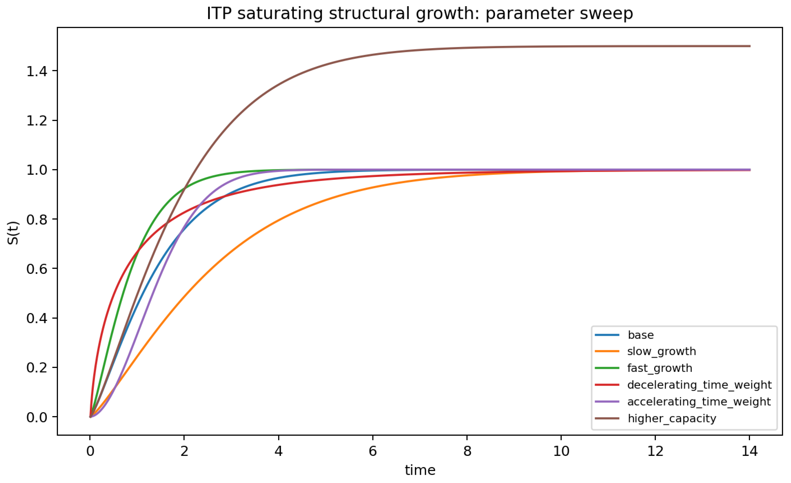
Figure 2. Validation of the auxiliary memory ODE against the direct Volterra convolution for the same exponential kernel. The small residual confirms that the local memory implementation used in simulations is faithful to the finite-memory convolution it is meant to represent.

Figure 2. Validation of the auxiliary memory ODE against the direct Volterra convolution for the same exponential kernel. The small residual confirms that the local memory implementation used in simulations is faithful to the finite-memory convolution it is meant to represent.

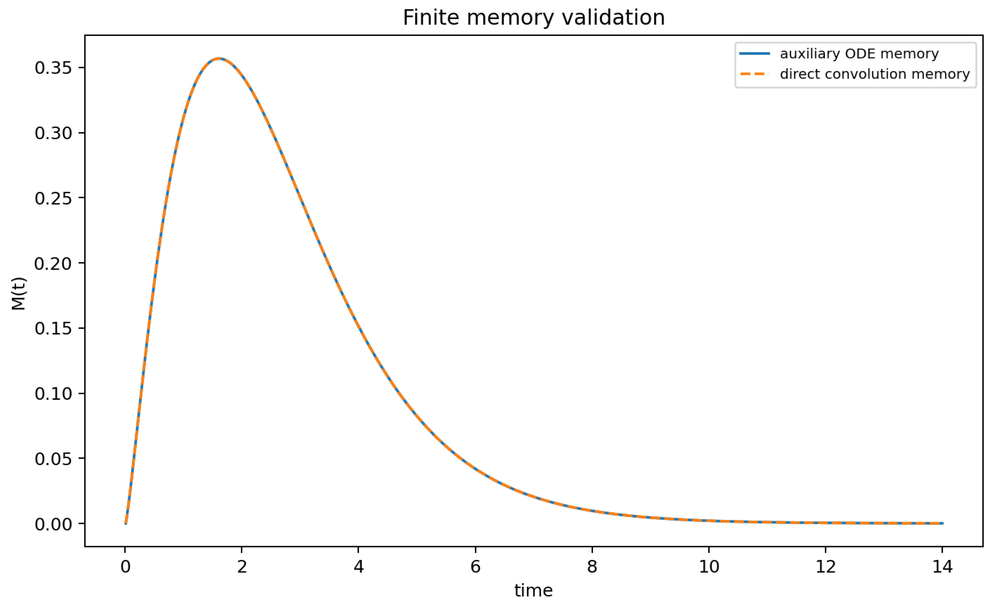
Figure 3. Cycle-filter inheritance test. The finite late-cycle residue recovers next-cycle parameters substantially better than shuffled-cycle nulls in this synthetic scaffold. This does not establish physical cyclic cosmology. It shows that cycle-to-cycle inheritance can be made operational through a finite filter and tested against explicit nulls.

Figure 3. Cycle-filter inheritance test. The finite late-cycle residue recovers next-cycle parameters substantially better than shuffled-cycle nulls in this synthetic scaffold. This does not establish physical cyclic cosmology. It shows that cycle-to-cycle inheritance can be made operational through a finite filter and tested against explicit nulls.

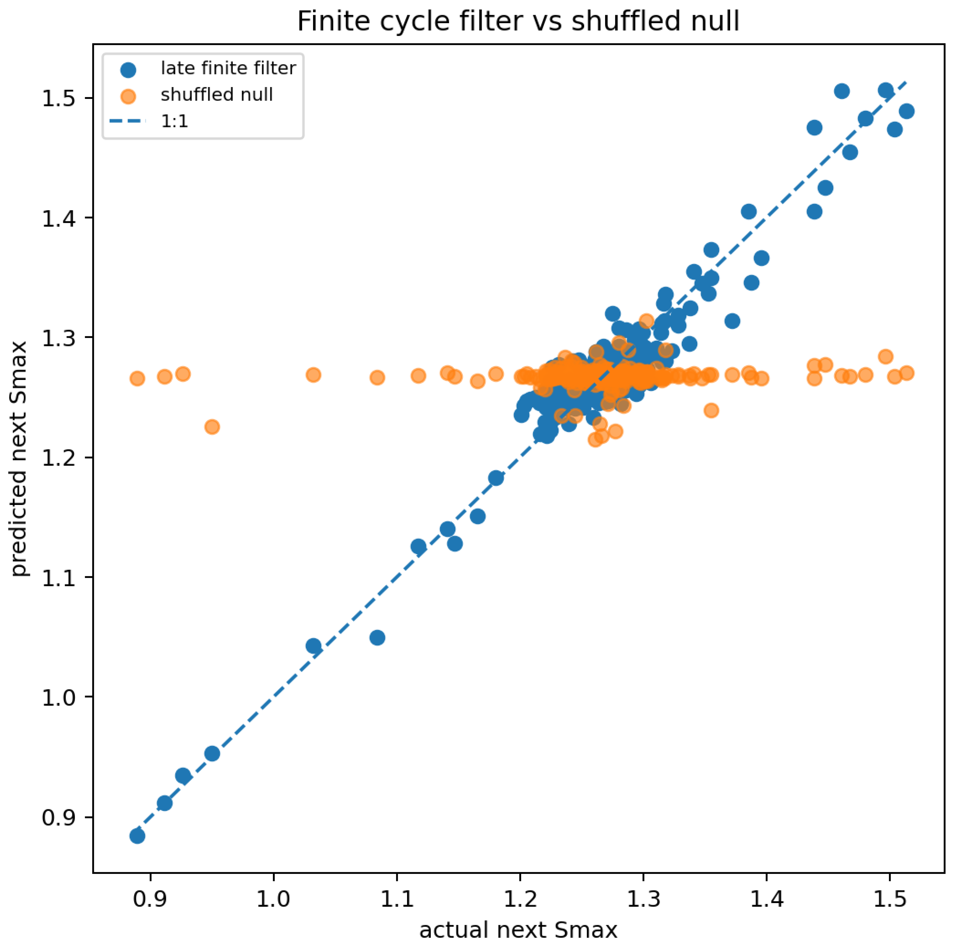
Figure 4. Synthetic trajectories of reduced ITP parameters across cycle index. The purpose of the plot is to visualize non-identical renewal: each finite sector remains inside the projected parameter range while carrying structured residue from previous sectors.

Figure 4. Synthetic trajectories of reduced ITP parameters across cycle index. The purpose of the plot is to visualize non-identical renewal: each finite sector remains inside the projected parameter range while carrying structured residue from previous sectors.

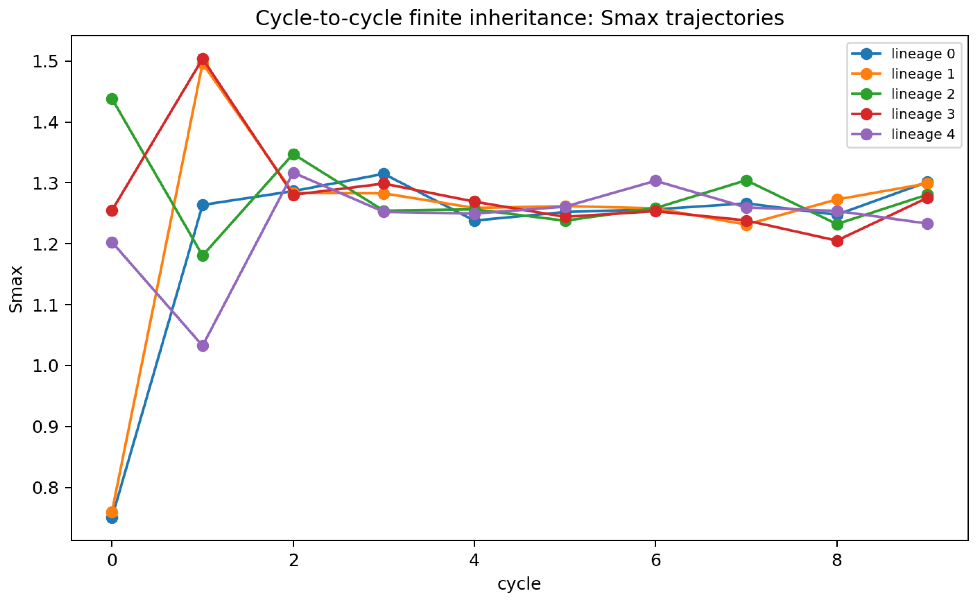
Figure 5. Filter-horizon sensitivity basin for synthetic cycle inheritance. The ripeness-weighted residue and the generic late structural residue remain far above the shuffled-cycle null over a broad interval of ${\Delta }_f$. The purpose is to test whether inheritance survives filter-horizon perturbation, not to claim physical cyclic cosmology.

Figure 5. Filter-horizon sensitivity basin for synthetic cycle inheritance. The ripeness-weighted residue and the generic late structural residue remain far above the shuffled-cycle null over a broad interval of ${\Delta }_f$. The purpose is to test whether inheritance survives filter-horizon perturbation, not to claim physical cyclic cosmology.

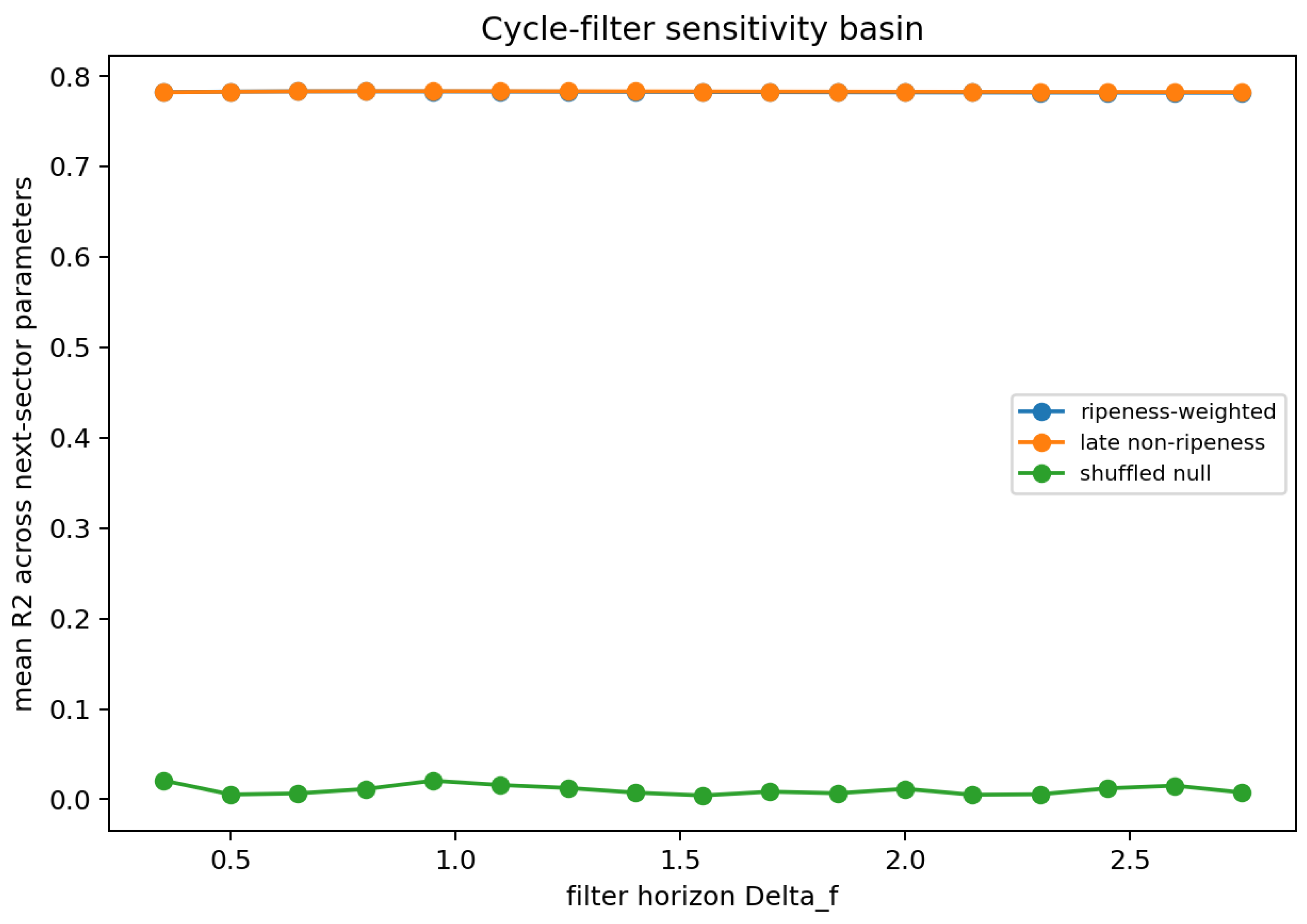
Table 1. Logical position of the present article within the broader ITP/CIOU series. The table is included to make the dependency structure explicit rather than hidden.

Component	Main function	Relation to present article
ITP parameter-space paper	Defines axioms A1-A5, finite memory horizon, saturating growth, seven-parameter manifold ${\mathcal{M}}_{\mathrm{ITP}}$, and reporting/falsification rules.	Supplies the finite local sector. This article does not redefine it.
Homeostatic-potential paper	Defines the structural code equation, archived homeostatic memory, code gain, homeostatic sovereignty, and structural commitment in HRSM language.	Supplies the finite inheritance constraint map. This article demotes the phrase “structural cosmic DNA” to a heuristic label for that code.
Arrow-of-time paper	Defines structural commitment as accumulated reshaping of accessible configuration space.	Supplies the directionality of finite-sector composition.
Bayesian Memory Ladder evidence paper	Tests restricted memory kernels against matched baselines under Bayesian evidence.	Used here only as a falsification gate, not as evidence for infinity.
Layered persistence geometry paper	Develops exoplanet persistence morphologies under adaptive, atmospheric, uncertainty, occupancy, and chemical-proxy constraints.	Supplies a local example of organic admissibility and measurement-aware ripeness without claiming life detection.
Present paper	Clarifies the word “infinite” as non-finality under finite memory and adds minimal robustness scaffolds.	Consolidates meaning, failure conditions, and toy transfer operators.

Table 1. Logical position of the present article within the broader ITP/CIOU series. The table is included to make the dependency structure explicit rather than hidden.

Component	Main function	Relation to present article
ITP parameter-space paper	Defines axioms A1-A5, finite memory horizon, saturating growth, seven-parameter manifold ${\mathcal{M}}_{\mathrm{ITP}}$, and reporting/falsification rules.	Supplies the finite local sector. This article does not redefine it.
Homeostatic-potential paper	Defines the structural code equation, archived homeostatic memory, code gain, homeostatic sovereignty, and structural commitment in HRSM language.	Supplies the finite inheritance constraint map. This article demotes the phrase “structural cosmic DNA” to a heuristic label for that code.
Arrow-of-time paper	Defines structural commitment as accumulated reshaping of accessible configuration space.	Supplies the directionality of finite-sector composition.
Bayesian Memory Ladder evidence paper	Tests restricted memory kernels against matched baselines under Bayesian evidence.	Used here only as a falsification gate, not as evidence for infinity.
Layered persistence geometry paper	Develops exoplanet persistence morphologies under adaptive, atmospheric, uncertainty, occupancy, and chemical-proxy constraints.	Supplies a local example of organic admissibility and measurement-aware ripeness without claiming life detection.
Present paper	Clarifies the word “infinite” as non-finality under finite memory and adds minimal robustness scaffolds.	Consolidates meaning, failure conditions, and toy transfer operators.

Table 2. Scope tiers used throughout the article. The present paper occupies Tiers 1 and 2. Tier 3 is deferred to branch-specific physical models.

Tier	Content	Status in this article
Tier 1	Semantic clarification: what “infinite”, “organic”, “cycle”, “inheritance”, and “ripeness” are allowed to mean.	Primary contribution.
Tier 2	Mathematical admissibility: finite memory, finite saturation, finite residue filters, null comparisons, and sensitivity gates.	Developed as minimal scaffolding.
Tier 3	Physical realization: branch-specific transfer operators, microphysical mechanisms, likelihoods, external observables, and empirical constraints.	Not derived here; required in later branch papers.

Table 2. Scope tiers used throughout the article. The present paper occupies Tiers 1 and 2. Tier 3 is deferred to branch-specific physical models.

Tier	Content	Status in this article
Tier 1	Semantic clarification: what “infinite”, “organic”, “cycle”, “inheritance”, and “ripeness” are allowed to mean.	Primary contribution.
Tier 2	Mathematical admissibility: finite memory, finite saturation, finite residue filters, null comparisons, and sensitivity gates.	Developed as minimal scaffolding.
Tier 3	Physical realization: branch-specific transfer operators, microphysical mechanisms, likelihoods, external observables, and empirical constraints.	Not derived here; required in later branch papers.

Table 3. Failure conditions for finite-memory non-finality claims.

Claim	Failure condition
Finite memory	The proposed memory term carries no predictive information beyond the current state and environment.
Structural inheritance code	The proposed structural constraint map does not constrain future trajectories, improve prediction, or survive perturbation.
Structural commitment	The commitment variable collapses into ordinary chronology, with no measurable alteration of reachable future states.
Cyclic renewal	The cycle reduces either to exact repetition or to random reset with no inherited constraint.
CIOU organic structure	The system shows no regulated persistence, no nested constraint, and no coherent memory-bearing dynamics.
Organic admissibility	The claimed organic structure reduces to mere life-existence, literal organismic metaphor, or proxy geometry that disappears under uncertainty propagation or independent validation.
Ripeness	Ripeness collapses into age, saturation, or persistence without recoverability; the ripeness-weighted residue performs no better than shuffled or random-reset residues.
Bayesian memory branch	The restricted memory sector fails evidence comparison against a matched baseline under converged and audited settings.

Table 3. Failure conditions for finite-memory non-finality claims.

Claim	Failure condition
Finite memory	The proposed memory term carries no predictive information beyond the current state and environment.
Structural inheritance code	The proposed structural constraint map does not constrain future trajectories, improve prediction, or survive perturbation.
Structural commitment	The commitment variable collapses into ordinary chronology, with no measurable alteration of reachable future states.
Cyclic renewal	The cycle reduces either to exact repetition or to random reset with no inherited constraint.
CIOU organic structure	The system shows no regulated persistence, no nested constraint, and no coherent memory-bearing dynamics.
Organic admissibility	The claimed organic structure reduces to mere life-existence, literal organismic metaphor, or proxy geometry that disappears under uncertainty propagation or independent validation.
Ripeness	Ripeness collapses into age, saturation, or persistence without recoverability; the ripeness-weighted residue performs no better than shuffled or random-reset residues.
Bayesian memory branch	The restricted memory sector fails evidence comparison against a matched baseline under converged and audited settings.

Table 4. Summary of saturating-growth robustness checks from the minimal run.

Check	Result	Interpretation
Monotonicity violations	0 across all settings	The tested trajectories respect pre-saturation monotone growth.
Largest analytic error	$4.45\times {10}^{-5}$	Numerical integration reproduces the analytic solution.
Base final saturation error	$8.79\times {10}^{-8}$	The base case approaches finite capacity.
Noisy parameter recovery	close to truth	Recovered $(\widehat{\alpha },\widehat{m},{\widehat{S}}_{max})\simeq (0.745,0.248,0.9998)$.

Table 4. Summary of saturating-growth robustness checks from the minimal run.

Check	Result	Interpretation
Monotonicity violations	0 across all settings	The tested trajectories respect pre-saturation monotone growth.
Largest analytic error	$4.45\times {10}^{-5}$	Numerical integration reproduces the analytic solution.
Base final saturation error	$8.79\times {10}^{-8}$	The base case approaches finite capacity.
Noisy parameter recovery	close to truth	Recovered $(\widehat{\alpha },\widehat{m},{\widehat{S}}_{max})\simeq (0.745,0.248,0.9998)$.

Table 5. Cycle-filter internal consistency results. $R^2$ values compare a finite late-cycle filter against early-filter, whole-cycle average, shuffled-cycle null, and mean-only baseline models.

Target	Late finite filter	Early filter	Whole-cycle average	Shuffled null	Mean-only
${\alpha }_{k+1}$	0.627	0.510	0.623	0.006	0.000
$m_{k+1}$	0.892	0.852	0.889	0.023	0.000
$S_{max,k+1}$	0.922	0.856	0.920	0.018	0.000
${\Delta }_{k+1}$	0.956	0.916	0.949	0.013	0.000

Table 5. Cycle-filter internal consistency results. $R^2$ values compare a finite late-cycle filter against early-filter, whole-cycle average, shuffled-cycle null, and mean-only baseline models.

Target	Late finite filter	Early filter	Whole-cycle average	Shuffled null	Mean-only
${\alpha }_{k+1}$	0.627	0.510	0.623	0.006	0.000
$m_{k+1}$	0.892	0.852	0.889	0.023	0.000
$S_{max,k+1}$	0.922	0.856	0.920	0.018	0.000
${\Delta }_{k+1}$	0.956	0.916	0.949	0.013	0.000

Table 6. Critical limitations and required response protocols.

Limitation	Risk	Required response
Integration bottleneck	Full ODE histories across many cycle boundaries become computationally prohibitive.	Use finite residue compression, recursive memory updates, cached kernels, and shuffled-cycle nulls.
Fossil-signal degeneracy	CMB or PBH anomalies are not unique to CIOU or ITP.	Use joint observables and competing null models; no single anomaly is decisive.
Ad-hoc bounce boundaries	Cycle-transfer operators may become symbolic placeholders.	Separate admissibility maps from physical bounce derivations; require branch-specific transfer maps.
Hyperparameter sensitivity	A result may survive only under tuned $\Delta$, $S_{max}$, or coupling values.	Report stability basins, profile likelihoods, sensitivity grids, and null comparisons.
Observational burden	Bayesian evidence gates require high-quality matched data.	Treat evidence as branch-level falsification, not proof of infinite transformation.
Organic/ripeness ambiguity	Organicity or ripeness may become a protected metaphor.	Define organic admissibility and ripeness functionals, then test them against uncertainty, shuffled residues, and independent observables.

Table 6. Critical limitations and required response protocols.

Limitation	Risk	Required response
Integration bottleneck	Full ODE histories across many cycle boundaries become computationally prohibitive.	Use finite residue compression, recursive memory updates, cached kernels, and shuffled-cycle nulls.
Fossil-signal degeneracy	CMB or PBH anomalies are not unique to CIOU or ITP.	Use joint observables and competing null models; no single anomaly is decisive.
Ad-hoc bounce boundaries	Cycle-transfer operators may become symbolic placeholders.	Separate admissibility maps from physical bounce derivations; require branch-specific transfer maps.
Hyperparameter sensitivity	A result may survive only under tuned $\Delta$, $S_{max}$, or coupling values.	Report stability basins, profile likelihoods, sensitivity grids, and null comparisons.
Observational burden	Bayesian evidence gates require high-quality matched data.	Treat evidence as branch-level falsification, not proof of infinite transformation.
Organic/ripeness ambiguity	Organicity or ripeness may become a protected metaphor.	Define organic admissibility and ripeness functionals, then test them against uncertainty, shuffled residues, and independent observables.

The scope boundary is simple: this article clarifies what infinite transformation, organic admissibility, and ripeness can mean inside a finite-memory formalism. It does not derive quantum-gravity bounce microphysics, does not prove cosmic cycles, and does not claim life detection. Those claims require branch-specific transfer operators and independent data.

15. Sharper Predictions

The original conceptual predictions are too broad unless tied to finite tests. The clarified framework therefore uses the following sharper expectations.

Prediction 1 

(Finite residue beats shuffled inheritance). A finite memory residue should predict next-sector parameters better than shuffled-cycle residues. If the shuffled null performs equally well, the cycle-inheritance claim fails.

Prediction 2 

(Exact recurrence is non-generic). Exact recurrence should fail as a generic cycle model. In a non-Markovian renewal framework, $p_{k+1}$ should not be statistically identical to $p_k$ except in a degenerate limit.

Prediction 3 

(Full history should not be necessary). A finite-memory implementation should not require the entire prior trajectory to predict the next sector. If only a full uncompressed archive works, the finite-memory version of ITP fails.

Prediction 4 

(Auxiliary and convolution memory must agree). The auxiliary ODE implementation and the direct Volterra convolution should agree numerically for the same kernel. If not, the localizable memory scaffold fails.

Prediction 5 

(Memory should not win everywhere). In physical branches, finite-memory models should outperform Markovian baselines where historical burden is expected to matter. If memory wins everywhere, the first suspicion should be overfitting, leakage, or poor baseline matching.

Prediction 6 

(Inheritance must survive sensitivity sweeps). A cycle-filter claim should remain positive over a nontrivial interval of ${\Delta }_f$. If ${\mathcal{R}}_{\mathrm{inherit}}\left({\Delta }_f\right)>0$ only at one tuned value, the claim is weak.

Prediction 7 

(Ripeness must add testable discipline). If ripeness is invoked as a technical variable, the ripeness-weighted residue must either improve prediction, improve stability, or provide a sharper failure classification than an unweighted late-history filter. Until that occurs, ripeness remains a candidate weighting principle rather than a validated universal variable.

15.0.0.1. Note on non-finality and falsification.

The non-finality claim is not directly falsified by a single finite observation, because no finite observation can prove absolute finality or infinite continuation. This is why the present article treats non-finality as a boundary interpretation rather than as a directly measured parameter. The falsifiable content lies in the finite projections: memory kernels, saturation laws, residue filters, organic-admissibility measures, ripeness weights, code-gain tests, null comparisons, and branch-level Bayesian evidence gates. If these finite projections fail repeatedly across the relevant branches, the physical use of the non-finality language loses support even though the abstract semantic claim is not directly measured. These predictions are intentionally modest. They do not claim that infinity has been observed. They state what must be true for finite-memory non-finality to remain technically meaningful.

16. Discussion

The word “infinite” survives only if it is stripped of unnecessary inflation. The local theory is finite. The memory horizon is finite. The saturation capacity is finite. The structural inheritance code is finite. The accessible homeostatic basin is finite. The empirical tests are finite.

The infinite claim concerns non-finality. It says that the end of a finite form is not equivalent to the end of transformation. A local identity may terminate, but its residual structure, matter, energy, constraint, or memory may become part of another admissible transformation sector.

This interpretation also keeps ITP coherent with the structural-cosmic-DNA metaphor without overloading it. The technical object is the structural inheritance code, a finite constraint map that must be instantiated separately in each branch. It is not a literal genome, not linguistic syntax, and not a claim that physical systems carry symbolic programs. It is a compact way to say that finite retained structure can constrain future admissibility without storing every event in the past.

The arrow of time then enters as structural commitment. The future is not open in an unconstrained sense. It is open inside the commitments created by prior transformation. The past survives not as a perfect archive, but as a deformation of future possibility.

CIOU follows naturally from this logic. A cycle is not a return to sameness. It is a renewal under inherited constraint. This avoids the fragile claim of exact recurrence and replaces it with a non-Markovian claim: each phase begins from the transformed residue of prior phases.

The robustness tests shift the paper’s posture. They do not prove the framework. They make the formalism operational enough to fail. The saturating growth law must approach $S_{max}$. The auxiliary memory equation must reproduce the convolution. The finite cycle filter must beat shuffled-cycle inheritance in synthetic null-separation tests. Branch-specific fossil claims must supply physical transfer maps before they can claim observational relevance. That is the discipline the framework needs.

Organicity and ripeness extend this same discipline. Organicity is not cosmic biology. It is regenerative admissibility: the capacity of a phase to generate nested persistence systems from material continuity, energy-gradient flow, bounded disequilibrium, memory, and recursive complexity. Ripeness is not intention. It is a candidate homeostatic-maturation weighting: a proposed way to mark HRSM balance without collapse into environmental domination, rigid entrenchment, or memory burden. Both concepts are allowed to fail, and ripeness remains a candidate until a physical branch shows that it adds information beyond late structural persistence.

The resulting position is provocative but not loose:

$$\begin{array}{|c|}\hline \mathrm{ITP}\mathrm{is}\mathrm{finite}\mathrm{in}\mathrm{every}\mathrm{local}\mathrm{model}\mathrm{and}\mathrm{infinite}\mathrm{only}\mathrm{in}\mathrm{its}\mathrm{refusal}\mathrm{of}\mathrm{absolute}\mathrm{finality}.\\ \hline\end{array}$$

17. Conclusions

The universe does not need to remember everything in order to keep transforming. It only needs finite memory with structural consequence.

The Infinite Transformation Principle should therefore be read as a finite-memory theory of non-finality. Each system remembers finitely, grows finitely, saturates finitely, and may die finitely. What does not follow is absolute finality. The end of a form is not the end of transformation.

The structural inheritance code names the finite constraint map through which the past remains generative. Structural commitment names the directional consequence through which the past becomes binding. CIOU names the larger cosmological envelope in which renewal occurs without exact repetition. Organic admissibility names the capacity of that envelope to generate localized persistence-bearing systems without requiring biological literalism. Ripeness names the homeostatic maturity of such systems when HRSM balance, recoverability, bounded memory, and viable future breadth are maintained.

The sharpest statement is:

Memory is finite, but transformation is non-final.

More fully:

All physical forms are finite expressions of an unclosed transformation process. They do not preserve the whole past, and they do not persist forever as themselves. They inherit enough structure to transform, and each transformation commits the future to a modified space of possibility.

That is the disciplined meaning of the infinite in the Infinite Transformation Principle and in the Cyclical Infinite Organic Universe.

References

- Atalebe, Stephen. The Parameter Space of the Infinite Transformation Principle: A Universal Framework for Irreversible Dynamics and Structural Memory . Draft Manuscr. 2026. [Google Scholar]
- Atalebe, Stephen. A Homeostatic Potential Formalism for Structural Memory and Cross-Scale System Persistence: An Effective-Action Theory of Structural Cosmic DNA . Draft manuscript. 2026.
- Atalebe, Stephen. The Arrow of Time as Accumulated Structural Commitment . Draft manuscript. 2026.
- Atalebe, Stephen. Bayesian Memory Ladder Evidence Report and Reply to Comment on Bayesian Inflationary Reconstructions from Planck 2018 Data . Draft evidence report, 2026. [Google Scholar]
- Atalebe, Stephen. Virialisangion as Viscosity: Deriving the ITP from TNG300 . Working manuscript, 2026. [Google Scholar]
- Atalebe, Stephen. A Universe Without Beginning: A Cyclical Infinite Organic Universe . In Book manuscript and associated theoretical notes; 2026. [Google Scholar]
- Atalebe, Stephen. Layered Persistence Geometries in Exoplanet Systems Under Adaptive and Atmospheric Coherence Constraints . Draft manuscript. 2026.
- Burbidge, E. Margaret; Burbidge, Geoffrey R.; Fowler, William A.; Hoyle, Fred. Synthesis of the elements in stars. Rev. Mod. Phys. 1957, 29, 547–650. [Google Scholar] [CrossRef]
- Cameron, Alastair G. W. Nuclear reactions in stars and nucleogenesis. Publ. Astron. Soc. Pac. 1957, 69, 201–222. [Google Scholar] [CrossRef]
- Kasting, James F.; Whitmire, Daniel P.; Reynolds, Ray T. Habitable zones around main sequence stars. Icarus 1993, 101, 108–128. [Google Scholar] [CrossRef] [PubMed]
- Falkowski, Paul G.; Barber, Richard T.; Smetacek, Victor. Biogeochemical controls and feedbacks on ocean primary production. Science 1998, 281, 200–206. [Google Scholar] [CrossRef] [PubMed]
- Boltzmann, Ludwig. Further studies on the thermal equilibrium of gas molecules. In Wiener Berichte; 1872. [Google Scholar]
- Bombelli, Luca; Lee, Joohan; Meyer, David; Sorkin, Rafael D. Space-time as a causal set. Phys. Rev. Lett. 1987, 59, 521–524. [Google Scholar] [CrossRef] [PubMed]
- Buchert, Thomas. On average properties of inhomogeneous fluids in general relativity: Dust cosmologies. General. Relativ. Gravit. 2000, 32, 105–125. [Google Scholar] [CrossRef]
- Crooks, Gavin E. Entropy production fluctuation theorem and the nonequilibrium work relation for free energy differences. Phys. Rev. E 1999, 60, 2721–2726. [Google Scholar] [CrossRef] [PubMed]
- Deser, S.; Woodard, R. P. Nonlocal cosmology. Phys. Rev. Lett. 2007, 99, 111301. [Google Scholar] [CrossRef] [PubMed]
- Deser, S.; Woodard, R. P. Nonlocal cosmology II: Cosmic acceleration without fine tuning or dark energy. J. Cosmol. Astropart. Phys. 2019, 2019(06), 034. [Google Scholar] [CrossRef]
- Jarzynski, Christopher. Nonequilibrium equality for free energy differences. Phys. Rev. Lett. 1997, 78, 2690–2693. [Google Scholar] [CrossRef]
- Koivisto, Tomi S. Dynamics of nonlocal cosmology. Phys. Rev. D. 2008, 77, 123513. [Google Scholar] [CrossRef]
- Maggiore, Michele; Mancarella, Michele. Nonlocal gravity and dark energy. Phys. Rev. D. 2014, 90, 023005. [Google Scholar] [CrossRef]
- Mori, Hazime. Transport, collective motion, and Brownian motion. Prog. Theor. Phys. 1965, 33(3), 423–455. [Google Scholar] [CrossRef]
- Penrose, Roger. Before the big bang: An outrageous new perspective and its implications for particle physics. Proceedings of EPAC 2006, Edinburgh, Scotland, 2006. [Google Scholar]
- Penrose, Roger. Cycles of Time: An Extraordinary New View of the Universe; Bodley Head: London, 2010. [Google Scholar]
- Penrose, Roger. The basic ideas of conformal cyclic cosmology. AIP Conf. Proc. 2012, 1446, 233–243. [Google Scholar] [CrossRef]
- Seifert, Udo. Stochastic thermodynamics, fluctuation theorems and molecular machines. Rep. Prog. Phys. 2012, 75, 126001. [Google Scholar] [CrossRef] [PubMed]
- Sorkin, Rafael D. Causal sets: Discrete gravity. In Lectures on Quantum Gravity; Springer, 2003; pp. pages 305–327. [Google Scholar]
- Volterra, Vito. Theory of Functionals and of Integral and Integro-Differential Equations; Dover Publications, 1959. [Google Scholar]
- Woodard, Richard P. Nonlocal models of cosmic acceleration. Found. Phys. 2014, 44, 213–233. [Google Scholar] [CrossRef]
- Zwanzig, Robert. Ensemble method in the theory of irreversibility. J. Chem. Phys. 1960, 33, 1338–1341. [Google Scholar] [CrossRef]
- Zwanzig, Robert. Memory effects in irreversible thermodynamics. Phys. Rev. 1961, 124, 983–992. [Google Scholar] [CrossRef]
- Zwanzig, Robert. Nonequilibrium Statistical Mechanics; Oxford University Press, 2001. [Google Scholar]
Disclaimer/Publisher’s Note: The statements, opinions and data contained in all publications are solely those of the individual author(s) and contributor(s) and not of MDPI and/or the editor(s). MDPI and/or the editor(s) disclaim responsibility for any injury to people or property resulting from any ideas, methods, instructions or products referred to in the content. |
© 2026 by the author. Licensee MDPI, Basel, Switzerland. This article is an open access article distributed under the terms and conditions of the Creative Commons Attribution (CC BY) license.
Copyright: This open access article is published under a Creative Commons CC BY 4.0 license, which permit the free download, distribution, and reuse, provided that the author and preprint are cited in any reuse.