Formulation of Thermodynamic Potentials Using Differential Forms with Natural Restrictions from Rheological (Spring–Dashpot) Networks

1. Introduction

Consider the following thought experiment. Write down a free-energy ansatz ${\varphi }_{\mathrm{frei}}=f({\epsilon }_{ij}^{\mathrm{rev}},D_i^{\mathrm{rev}},\theta ,\left\{\iota \right\})$ for a coupled electro-thermo-mechanical material, expand its total differential, and combine the result with the energy balance. The reversible work contributions ought to cancel against those of the inner energy, leaving only the irreversible terms. They do not. A residual term of the form $-(\partial {\varphi }_{\mathrm{frei}}/\partial \left\{\iota \right\})\dot{\iota }$ survives, and the dissipation rate so obtained contradicts the work pairing of the inner energy [2]. The trouble is not the integration; the trouble is that $(\epsilon ,D,\theta )$ are not jointly the natural variables of any single thermodynamic potential reachable from the inner energy by a Legendre transformation in entropy alone. The variables have to be chosen in a way that is compatible with the work pairing they inherit — and that compatibility cannot be read off the constitutive ansatz itself.

The main result of this paper is the following. On a star-shaped reversible state space, the constitutive Jacobian of the rheological replacement model is symmetric if and only if a thermodynamic potential exists; that symmetry is, in coupled-field problems, the family of Maxwell relations between the coupled effects (Theorem 1 and Corollary 1). The reversible coordinate of each branch is its elastic spring strain; Hooke’s law on that strain assembles the constitutive 1-form, and the natural variables of the inner energy reappear when the non-elastic sub-strains of each branch are substituted by their own constitutive laws – a step that emerges naturally in the worked example of Section 5 and is not a separate axiom. The thermodynamic potential itself, the full constitutive set, and Truesdell’s principle of equipresence follow without further postulates; the residual dissipation inequality appears as the remaining part of the Clausius–Duhem inequality after all process-independent contributions have been absorbed into the potential. The specification of a positive dissipative kinetics ($\eta >0$ for dashpots and analogous positivity conditions for plastic flows or ohmic resistors) is independent of the present framework and is invoked only once, in Section 5, as a concrete instance. The Poincaré lemma is classical; the content of the paper is the construction upstream of it, the map

$$\underset{\mathrm{rheological}\mathrm{network}}{\underbrace{M}}⟶\underset{\mathrm{constitutive}1-\mathrm{form}}{\underbrace{\omega =\langle {\zeta }_{\alpha },\mathrm{d}{\xi }^{\alpha }\rangle }}⟶\underset{\mathrm{closedness}=\mathrm{Maxwell}}{\underbrace{{\zeta }_{\alpha ;\beta }={\zeta }_{\beta ;\alpha }^{\top }}}⟶\underset{\mathrm{potential}}{\underbrace{\phi }},$$

by which a rheological diagram becomes a constitutive 1-form whose closedness coincides with a physically familiar set of identities.

The construction is complementary to the internal-variable framework of Coleman and Gurtin [9], the GENERIC formalism of Grmela, Öttinger and Mielke [10,11,12], the port-Hamiltonian view of van der Schaft and Maschke [14], and the energetic / polyconvex free-energy constructions of e.g. [3,4]: these address the admissible structure of the potential once the variables are given, while the present contribution operates one step upstream, at the choice of variables itself.

2. Notation

Let $S={⨁}_{\alpha =1}^A{V}_{\alpha }$ be a finite-dimensional inner-product space written as a direct sum of tensor slots $V_{\alpha }$, each carrying one independent reversible state coordinate ${\xi }_{\alpha }\in V_{\alpha }$, and let $G\subset S$ be a star-shaped open domain. A constitutive operator on G is a smooth map $\zeta :G\to S^{*}$ with components ${\zeta }_{\alpha }\left(\xi \right)\in V_{\alpha }^{*}$ paired with state increments by $\langle \zeta \left(\xi \right),\delta \xi \rangle ={\sum }_{\alpha }\langle {\zeta }_{\alpha },\delta {\xi }_{\alpha }\rangle$. Its first variation is the constitutive Jacobian,

$$\mathsf{J}\left(\xi \right)={\left[{\zeta }_{\alpha ;\beta }\left(\xi \right)\right]}_{\alpha ,\beta =1}^A,{\zeta }_{\alpha ;\beta }:={\displaystyle \frac{\partial {\zeta }_{\alpha }}{\partial {\xi }_{\beta }}}\in V_{\alpha }^{*}\otimes V_{\beta }^{*},$$

(1)

and the associated constitutive 1-form on G is $\omega :=\langle {\zeta }_{\alpha },\mathrm{d}{\xi }^{\alpha }\rangle$. The slot decomposition $S=⨁V_{\alpha }$ is here a notational vehicle; which slots actually appear in the construction is the question addressed in Section 3. The semicolon in ${\zeta }_{\alpha ;\beta }$ denotes the constitutive derivative and is distinct from the comma for spatial derivatives.

3. From Rheological Models to Constitutive Operators

A rheological replacement model M is a finite forest of branches in parallel, each branch a serial chain of components. A spring within branch i carries the elastic strain ${\epsilon }^{\left(i\right),e}$; by Hooke’s law, the branch stress is a linear function of ${\epsilon }^{\left(i\right),e}$, and the serial arrangement of the branch forces the same stress through every other component of the branch. The elastic strain ${\epsilon }^{\left(i\right),e}$ is therefore the natural reversible coordinate of branch i, and the constitutive 1-form is assembled on the tuple ${\epsilon }^{\left(\right),e}=({\epsilon }^{\left(1\right),e},\dots ,{\epsilon }^{\left(I\right),e})$ alone. The remaining sub-strains contributed by the other components of each branch (thermal, electric, viscous, plastic, …) and the way they re-introduce the natural variables of the inner energy through their own constitutive laws are model-specific and are addressed inside the worked example of Section 5. The slot decomposition $S={⨁}_{\alpha }{V}_{\alpha }$ of Section 2 is the output of that construction, not its input.

3.1. Physical Effects and the Reduction Lemma

A physical effect attached to M is a triple $(V_{\alpha },{\xi }_{\alpha },{\zeta }_{\alpha })$: a tensor slot $V_{\alpha }$ corresponding to a component (or coupled subset of components) of M, an independent reversible state coordinate ${\xi }_{\alpha }\in V_{\alpha }$, and a constitutive law ${\zeta }_{\alpha }:G_{\mathrm{rev}}\to V_{\alpha }^{*}$ whose column in $\mathsf{J}$ is supported only at the rows of effects coupled to $\alpha$ in the topology of M. The model is complete on $G_{\mathrm{rev}}$ if every reversible coordinate of every component is the $\xi$-coordinate of exactly one such effect.

Lemma 1 

(reduction). Let M be a complete rheological model on $G_{\mathrm{rev}}$ with I branches in series–parallel arrangement, and assume that each branch contributes exactly one independent reversiblebranch coordinateafter the serial compatibility constraints have been enforced. Then within each branch the constitutive laws of all components reduce to a single branch-stress equation, and the constitutive operator ζ on $G_{\mathrm{rev}}$ is square of size $A=I$.

Proof. 

Within a branch, serial arrangement enforces equality of the branch stress; the per-component laws become mutually equivalent and can be replaced by a single representative. Parallel arrangement across branches preserves independence of effects. The total number of independent constitutive equations equals I. □

Remark 1. 

The single-coordinate hypothesis of Lemma 1 is satisfied by the present class of spring–dashpot replacement models; branches that carry several independent reversible coordinates (e.g. an electromechanical branch with an additional dielectric slot) contribute one stress equation per such coordinate, and the size of ζ grows accordingly. The hybrid model of Section 5 is treated as a concrete instance of the latter situation: Branch 1 carries three reversible coordinates and contributes the dense upper-left $3\times 3$ block of $\mathsf{J}$, while Branch 2 contributes the single viscous block, with $A=4$ rather than $A=2$.

4. Main Theorem

Theorem 1 

(constructive existence of the potential). Let M be a complete rheological model on a star-shaped domain $G_{\mathrm{rev}}\subset S$ and let $\zeta \in C^1(G_{\mathrm{rev}},S^{*})$ be its constitutive operator, as constructed in Section 3. The following are equivalent:

(i) 

the constitutive Jacobian $\mathsf{J}$ is symmetric on $G_{\mathrm{rev}}$,

$${\zeta }_{\alpha ;\beta }\left(\xi \right)={\zeta }_{\beta ;\alpha }{\left(\xi \right)}^{\top }\forall \alpha ,\beta ,\forall \xi \in G_{\mathrm{rev}};$$

(2)

(ii) 

there exists a thermodynamic potential $\phi \in C^2(G_{\mathrm{rev}},\mathbb{R})$, unique up to an additive constant, such that ${\zeta }_{\alpha }=\partial \phi /\partial {\xi }_{\alpha }$ for all $\alpha =1,\dots ,A$.

A primitive is provided by the homotopy formula anchored at a star-centre ${\xi }^0\in G_{\mathrm{rev}}$,

$$\phi \left(\xi \right)-\phi \left({\xi }^0\right)={\int }_0^1〈{\zeta }_{\alpha }\left({\xi }^0+t(\xi -{\xi }^0)\right),{\xi }^{\alpha }-{\xi }^{0,\alpha }〉\mathrm{d}t.$$

(3)

The entire constitutive set is recovered by differentiation of φ, and Truesdell’s principle of equipresence is automatic.

Proof. 

By construction, $\zeta$ maps the reversible state space S into its dual $S^{*}$, so the constitutive Jacobian $\mathsf{J}$ is square on $G_{\mathrm{rev}}$; Lemma 1 gives the corresponding explicit reduction in the single-coordinate branch case. Closedness of $\omega =\langle {\zeta }_{\alpha },\mathrm{d}{\xi }^{\alpha }\rangle$ reads, in coordinates, ${\zeta }_{\alpha ;\beta }-{\zeta }_{\beta ;\alpha }^{\top }=0$, i.e. (2). By the Poincaré lemma on a star-shaped domain every closed 1-form is exact; the homotopy formula (3) provides a primitive, and uniqueness up to an additive constant follows from connectedness. □

Corollary 1 

(emergent Maxwell relations). Under the hypotheses of Theorem 1, every off-diagonal block of $\mathsf{J}$ that corresponds to two physically distinct effects coupled in M is the Maxwell relation between the conjugate pairs $({\xi }_{\alpha },{\zeta }_{\alpha })$ and $({\xi }_{\beta },{\zeta }_{\beta })$:

$${\displaystyle \frac{\partial {\zeta }_{\alpha }}{\partial {\xi }_{\beta }}}={\left({\displaystyle \frac{\partial {\zeta }_{\beta }}{\partial {\xi }_{\alpha }}}\right)}^{\top }.$$

(4)

Proof. 

By Theorem 1 the entries of $\mathsf{J}$ are the second derivatives ${\partial }^2\phi /\partial {\xi }_{\alpha }\partial {\xi }_{\beta }$ and Schwarz’s theorem applies. □

5. A Hybrid Electro-Thermo-Viscoelastic Model

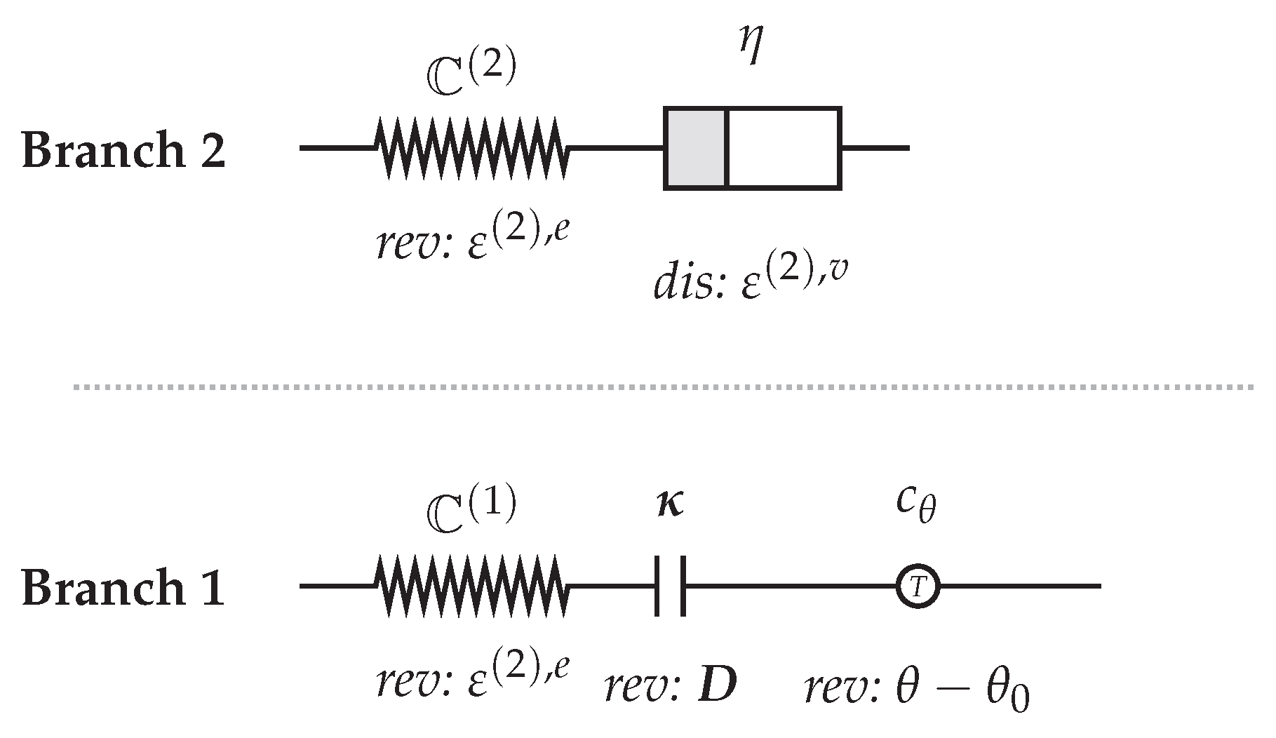
To exhibit more than the textbook quadratic case, we consider a two-branch hybrid model, according to Figure 1, in which one branch carries a viscoelastic Maxwell internal variable and the other branch couples elasticity, piezoelectricity, thermoelasticity, and pyroelectricity. The construction must therefore handle electromechanical coupling, an internal variable, dissipative branch splitting, and the emergence of several Maxwell relations simultaneously.

5.1. Structure of the Replacement Model

Branch 1 (elastic–piezoelectric–thermoelastic). A linear spring with elasticity tensor ${\mathbb{C}}^{\left(2\right)}$, a dielectric capacitance with reciprocal permittivity tensor $\kappa$, and a calorimetric component with specific heat $c_{\theta }$ at reference temperature ${\theta }_0$. Cross-couplings are encoded by the piezoelectric tensor $\mathit{e}$, the thermoelastic stress tensor $\beta$, and the pyroelectric vector $\mathit{p}$ (notation as in [2]).

Branch 2 (viscoelastic Maxwell). A linear spring with elasticity tensor ${\mathbb{C}}^{\left(1\right)}$ in series with a linear dashpot of viscosity $\eta$. The branch strain decomposes additively,

$${\epsilon }^{\left(2\right)}={\epsilon }^{\left(2\right),e}+{\epsilon }^{\left(2\right),v},$$

(5)

with elastic part ${\epsilon }^{\left(2\right),e}$ as the reversible coordinate and viscous part ${\epsilon }^{\left(2\right),v}$ as the dissipative internal variable. The schematic of M is given in Figure 1.

5.2. Stage 1: Stored Energy in Pure Elastic-Strain Coordinates

We first apply Hooke’s law to each branch. The branch stresses are ${\sigma }^{\left(1\right)}={\mathbb{C}}^{\left(2\right)}{\epsilon }^{\left(1\right),e}$ and ${\sigma }^{\left(2\right)}={\mathbb{C}}^{\left(1\right)}{\epsilon }^{\left(2\right),e}$, and the total stress is the sum $\sigma ={\sigma }^{\left(1\right)}+{\sigma }^{\left(2\right)}$. The corresponding constitutive 1-form on the pure elastic-strain space is

$${\omega }^{\left(\mathrm{I}\right)}={\sigma }^{\left(1\right)}:\mathrm{d}{\epsilon }^{\left(1\right),e}+{\sigma }^{\left(2\right)}:\mathrm{d}{\epsilon }^{\left(2\right),e}.$$

(6)

Hooke’s law makes the constitutive Jacobian of ${\omega }^{\left(\mathrm{I}\right)}$ block-diagonal with entries ${\mathbb{C}}^{\left(2\right)},{\mathbb{C}}^{\left(1\right)}$; the symmetry of the elasticity tensors makes it symmetric, so Theorem 1 applies and the homotopy formula (3) with ${\xi }^0=0$ produces the Stage-1 stored energy

$$u_0\left({\epsilon }^{\left(1\right),e},{\epsilon }^{\left(2\right),e}\right)=\frac{1}{2}{\epsilon }^{\left(1\right),e}:{\mathbb{C}}^{\left(2\right)}{\epsilon }^{\left(1\right),e}+\frac{1}{2}{\epsilon }^{\left(2\right),e}:{\mathbb{C}}^{\left(1\right)}{\epsilon }^{\left(2\right),e}.$$

(7)

This is exactly the elastic potential of [2]. It contains no electric, thermal, or viscous variable yet; those enter in Stage 2.

5.3. Stage 2a: Additive Strain Decomposition of Each Branch

The rheological topology of each branch constrains its elastic strain algebraically. For the present hybrid model these constraints read (cf. [2])

$${\epsilon }^{\left(1\right),e}=\epsilon -{\epsilon }^{\mathrm{th}}-{\epsilon }^{\mathrm{el}}-{\epsilon }^{\left(1\right),\mathrm{irr}},{\epsilon }^{\left(2\right),e}=\epsilon -{\epsilon }^{\left(2\right),v},$$

(8)

where $\epsilon$ is the (common) total strain of the two parallel branches and ${\epsilon }^{\mathrm{th}},{\epsilon }^{\mathrm{el}},{\epsilon }^{\left(1\right),\mathrm{irr}},{\epsilon }^{\left(2\right),v}$ are the thermal, electric (piezoelectric), plastic, and viscous sub-strains. The internal variables $({\epsilon }^{\left(1\right),\mathrm{irr}},{\epsilon }^{\left(2\right),v})$ parametrize dissipative components and are independent of the external loading; they evolve in time according to flow rules derived below.

5.4. Stage 2b: Taylor Expansion of the Reversible Sub-Strains

The thermal and electric sub-strains are themselves functions of the state. A first-order Taylor expansion around a reference state (entropy $s_0$, dielectric displacement $\mathit{D}=0$) yields

$${\epsilon }^{\mathrm{th}}=b^u\Delta s,{\epsilon }^{\mathrm{el}}={\tilde{d}}^u{\mathit{D}}^{\mathrm{rev}},$$

(9)

with $\Delta s=s-s_0$ and material tensors $b^u$ (thermal expansion at constant elastic strain) and ${\tilde{d}}^u$ (piezoelectric strain coefficient). The choice of $\Delta s$ as the expansion variable for ${\epsilon }^{\mathrm{th}}$ – and not$\Delta T$ – is forced by the requirement that the substituted potential be consistent with the inner energy under Legendre transformation: $(s,\Delta s)$ and not $(T,\Delta T)$ is the variable conjugate to the thermal stress in the work pairing of (6). The same argument selects ${\mathit{D}}^{\mathrm{rev}}$ (rather than $\mathit{E}$) as the expansion variable of ${\epsilon }^{\mathrm{el}}$. The detailed justification is in [2]; choosing the conjugate variables (T instead of s, $\mathit{E}$ instead of $\mathit{D}$) produces the spurious dissipation rate of [2].

5.5. Stage 2c: Substituted Potential and Material Tensors

Substituting (8)–(9) into (7) and collecting terms with the standard definitions of the thermal stress coefficient ${\omega }^u=-{\mathbb{C}}^{\left(2\right)}{b}^u$,1 the piezoelectric coupling ${\mathsf{\Lambda }}^u=-{\mathbb{C}}^{\left(2\right)}{\tilde{d}}^u$, the dielectric coefficient ${\mathsf{\Omega }}^u$, the pyroelectric vector ${\mathit{p}}^u$ and the heat-capacity scalar ${\mathsf{\Gamma }}^u$ (cf. [2]), the substituted potential reads

$$\begin{array}{cc}\hfill u(\xi ,\gamma )=& \frac{1}{2}\left(\epsilon -{\epsilon }^{\left(1\right),\mathrm{irr}}\right):{\mathbb{C}}^{\left(2\right)}\left(\epsilon -{\epsilon }^{\left(1\right),\mathrm{irr}}\right)+{\omega }^u:\left(\epsilon -{\epsilon }^{\left(1\right),\mathrm{irr}}\right)\Delta s\hfill \\ \hfill & +{\mathsf{\Lambda }}^u:\left(\epsilon -{\epsilon }^{\left(1\right),\mathrm{irr}}\right)\left(\mathit{D}-{\mathit{P}}^{\left(1\right),\mathrm{irr}}\right)+\frac{1}{2}{\mathsf{\Gamma }}^u{(\Delta s)}^2\hfill \\ \hfill & +\frac{1}{2}\left(\mathit{D}-{\mathit{P}}^{\left(1\right),\mathrm{irr}}\right)·{\mathsf{\Omega }}^u\left(\mathit{D}-{\mathit{P}}^{\left(1\right),\mathrm{irr}}\right)+p^u·\left(\mathit{D}-{\mathit{P}}^{\left(1\right),\mathrm{irr}}\right)\Delta s\hfill \\ \hfill & +\frac{1}{2}\epsilon :{\mathbb{C}}^{\left(1\right)}\epsilon +\frac{1}{2}{\epsilon }^{\left(2\right),v}:{\mathbb{C}}^{\left(1\right)}{\epsilon }^{\left(2\right),v}-{\epsilon }^{\left(2\right),v}:{\mathbb{C}}^{\left(1\right)}\epsilon ,\hfill \end{array}$$

(10)

which is exactly [2]. The natural external variables collected in $\xi$ are $(\epsilon ,s,\mathit{D})$; the internal variables collected in $\gamma$ are $({\epsilon }^{\left(1\right),\mathrm{irr}},{\mathit{P}}^{\left(1\right),\mathrm{irr}},{\epsilon }^{\left(2\right),v})$. ${\epsilon }^{\left(1\right),\mathrm{irr}}$ and ${\mathit{P}}^{\left(1\right),\mathrm{irr}}$ can also expressed by a conjunct internal variable, see Appendix A. The potential $u(\xi ,\gamma )$ depends on both. We emphasise that ${\epsilon }^{\left(2\right),v}$ appears in u – this is essential for what follows.

The induced constitutive operator $\zeta =\partial u/\partial (\xi ,\gamma )$ has the block-diagonal structure of [2]: the four-dimensional $(\epsilon ,\mathit{D},s,{\epsilon }^{\left(2\right),v})$ Jacobian

$$\mathsf{J}=\left(\begin{array}{cccc}{\mathbb{C}}^{\left(2\right)}& {\mathsf{\Lambda }}^u& {\omega }^u& 0\\ {\left({\mathsf{\Lambda }}^u\right)}^{\top }& {\mathsf{\Omega }}^u& p^u& 0\\ {\left({\omega }^u\right)}^{\top }& {\left(p^u\right)}^{\top }& {\mathsf{\Gamma }}^u& 0\\ 0& 0& 0& {\mathbb{C}}^{\left(1\right)}\end{array}\right).$$

(11)

The dense upper-left $3\times 3$ block carries the piezoelectric, thermoelastic, and pyroelectric couplings of Branch 1; the lower-right entry ${\mathbb{C}}^{\left(1\right)}$ is the second-derivative ${\partial }^{2}u/\partial {\left({\epsilon }^{\left(2\right),v}\right)}^2$ that governs the dynamics of the viscous internal variable of Branch 2, as derived below. The internal variables $({\epsilon }^{\left(1\right),\mathrm{irr}},{\mathit{P}}^{\left(1\right),\mathrm{irr}})$ enter (10) only through the combinations $\epsilon -{\epsilon }^{\left(1\right),\mathrm{irr}}$ and $\mathit{D}-{\mathit{P}}^{\left(1\right),\mathrm{irr}}$ and contribute no independent block to $\mathsf{J}$; they evolve through their own flow rules (see [2]).

5.6. Emergent Maxwell Relations

Symmetry of $\mathsf{J}$ in (11) – the integrability condition of Theorem 1 – is equivalent to the following structural identities, none of which is separately postulated:

$$\begin{array}{cccc}\hfill {\displaystyle \frac{\partial \sigma }{\partial \mathit{D}}}& ={\mathsf{\Lambda }}^u={\left({\displaystyle \frac{\partial \mathit{E}}{\partial \epsilon }}\right)}^{\top }\hfill & \hfill & (\mathrm{piezoelectric}\mathrm{Maxwell}\mathrm{relation}),\hfill \end{array}$$

(12)

$$\begin{array}{cccc}\hfill {\displaystyle \frac{\partial \sigma }{\partial s}}& ={\omega }^u={\left({\displaystyle \frac{\partial \theta }{\partial \epsilon }}\right)}^{\top }\hfill & \hfill & (\mathrm{thermoelastic}\mathrm{Maxwell}\mathrm{relation}),\hfill \end{array}$$

(13)

$$\begin{array}{cccc}\hfill {\displaystyle \frac{\partial \mathit{E}}{\partial s}}& =p^u={\displaystyle \frac{\partial \theta }{\partial \mathit{D}}}\hfill & \hfill & (\mathrm{pyroelectric}\mathrm{Maxwell}\mathrm{relation}).\hfill \end{array}$$

(14)

Each is a single off-diagonal block of the $3\times 3$ Jacobian of the natural reversible variables $(\epsilon ,\mathit{D},s)$ being equal to the transpose of its mirror image. The construction produces all three at once – and, by Corollary 1, this generalises to any further coupled field that may be adjoined.

5.7. Driving Forces and Dissipation

The Stage-2 potential $u(\xi ,\gamma )$ depends on the viscous variable ${\epsilon }^{\left(2\right),v}$. Its partial derivative identifies the thermodynamic driving force of that variable,

$$Y_{{\epsilon }^{\left(2\right),v}}:=-{\displaystyle \frac{\partial u}{\partial {\epsilon }^{\left(2\right),v}}}={\mathbb{C}}^{\left(1\right)}\left(\epsilon -{\epsilon }^{\left(2\right),v}\right)={\sigma }^{\left(2\right)},$$

(15)

in agreement with [2]. The residual dissipation rate associated with that variable is then the remaining contribution to the Clausius–Duhem inequality after the process-independent terms have been absorbed into u,

$${\mathcal{D}}_{\mathrm{res}}=-{\displaystyle \frac{\partial u}{\partial {\epsilon }^{\left(2\right),v}}}:\dot{{\epsilon }^{\left(2\right),v}}=Y_{{\epsilon }^{\left(2\right),v}}:\dot{{\epsilon }^{\left(2\right),v}}.$$

(16)

The potential supplies the driving force and the residual structure; non-negativity of ${\mathcal{D}}_{\mathrm{res}}$ requires a separate positive dissipative kinetic law. For the specific linear dashpot ansatz ${\sigma }^{\left(2\right)}=\eta \dot{{\epsilon }^{\left(2\right),v}}$ with $\eta >0$ one recovers the Maxwell evolution $\eta \dot{{\epsilon }^{\left(2\right),v}}={\mathbb{C}}^{\left(1\right)}(\epsilon -{\epsilon }^{\left(2\right),v})$ and, as an illustration,

$${\mathcal{D}}_{\mathrm{res}}=\eta |\dot{{\epsilon }^{\left(2\right),v}}{|}^2\ge 0,$$

(17)

but the framework itself stops one step earlier, at the identification of the driving force and the residual. The same applies to the internal variables $({\epsilon }^{\left(1\right),\mathrm{irr}},{\mathit{P}}^{\left(1\right),\mathrm{irr}})$ of Branch 1: their thermodynamic driving forces $-\partial u/\partial {\epsilon }^{\left(1\right),\mathrm{irr}}$ and $-\partial u/\partial {\mathit{P}}^{\left(1\right),\mathrm{irr}}$ are read off from u; the corresponding flow rules are subject to the experimentally motivated kinematic hardening laws of [2].

More generally, the viscous contribution is only one residual term. If the irreversible strain and polarization are themselves resolved by additional internal variables ${\alpha }_a$, i.e.

$${\epsilon }_{ij}^{\mathrm{irr}}={\epsilon }_{ij}^{\mathrm{irr}}\left({\alpha }_a\right),P_i^{\mathrm{irr}}=P_i^{\mathrm{irr}}\left({\alpha }_a\right),$$

then the residual Clausius–Duhem contribution contains further terms of the form

$${\mathcal{D}}_{\mathrm{res}}=Y_{{\epsilon }^{\left(2\right),v}}:{\dot{\epsilon }}^{\left(2\right),v}+\sum _a{Y}_{{\alpha }_a}{\dot{\alpha }}_a,Y_{{\alpha }_a}:=-{\displaystyle \frac{\partial u}{\partial {\alpha }_a}}.$$

Thus the potential identifies the conjugate driving forces not only for the viscous strain, but also for any lower-level internal variable by which irreversible strain, irreversible polarization, or evolving material coefficients are represented. A concrete ferroelectric realization of this structure, based on domain volume fractions, is recalled in Appendix A.

5.8. Stored Energy in the Variables of the Free Energy

A Legendre transformation of u in $(\mathit{D},s)\mapsto (\mathit{E},-T)$ produces the free energy $\psi$ in the natural variables $(\epsilon ,\mathit{E},T,{\epsilon }^{\left(1\right),\mathrm{irr}},{\mathit{P}}^{\left(1\right),\mathrm{irr}},{\epsilon }^{\left(2\right),v})$. The framework guarantees that $\psi$ is consistent with u because the Legendre transformation acts on the natural variables identified by Stage 2b, not on an ad-hoc subset. Convexity of u is equivalent to positive-definiteness of the block matrix in (11) and is shown in [2].

5.9. Take-Away

This example shows that the framework does more than reproduce quadratic elasticity. A single integrability statement on a $4\times 4$ constitutive Jacobian organizes electromechanical coupling, thermoelasticity, pyroelectricity, and a viscoelastic internal variable within a common constructive scheme; all three Maxwell relations emerge simultaneously; and the residual form of the dissipation inequality is obtained as the remaining Clausius–Duhem contribution after the process-independent terms have been absorbed into the potential, rather than being imposed at the level of the reversible constitutive set.

6. Conclusion

The rheological replacement model of a coupled-field material fixes the natural variables of its thermodynamic potential, and the existence of the potential reduces to a single symmetry condition on the constitutive Jacobian. In the hybrid electro-thermo-viscoelastic example that condition encodes the piezoelectric, thermoelastic, and pyroelectric Maxwell relations simultaneously, and the residual form of the Clausius–Duhem inequality is obtained after the process-independent contributions have been absorbed into the potential; for the linear dashpot ansatz that residual reduces to a positive quadratic rate.

Three caveats delineate the boundary of validity. First, Theorem 1 delivers a hyperelastic stored-energy potential on the reversible coordinates $G_{\mathrm{rev}}$; the full Helmholtz or Gibbs free energy requires a Legendre transformation, and the identification of the underlying potential (inner energy, Helmholtz, enthalpy, …) is a modelling decision upstream of the algorithm. Second, star-shapedness of $G_{\mathrm{rev}}$ mattersfor the construction of a global primitive. For small-strain mechanics the state space is linear and star-shaped about any interior point, so the question does not arise. For finite kinematics the construction still applies on any star-shaped (Hencky-logarithmic) chart of ${\mathrm{GL}}^{+}\left(3\right)$ which is the standard local chart in finite-strain implementations – and the question of a global extension across the manifold of multiplicative decompositions $\mathit{F}={\mathit{F}}^e{\mathit{F}}^p$ is one of local-to-global care, not a failure of the framework. Genuine de Rham obstructions arise only for state spaces with non-trivial first cohomology – periodic crystallographic angles, multiply-connected phase configurations, and similar – in which case the multivalued primitive carries an interpretable topological charge. The topological discussion is collected in Appendix B. Third, the approach is bottom-up and natural for materials with a developed rheological analogue; for compressible fluids, reactive or phase-field media, a disciplined top-down ansätz controlled by the Legendre structure may remain preferable.

Appendix B.1. Star-Shaped Versus Contractible.

Star-shapedness is the simplest sufficient condition for exactness of closed 1-forms via the explicit homotopy formula (3). The Poincaré lemma itself requires only contractibility (the identity of the domain homotopic to a constant map); star-shapedness implies contractibility, but not conversely. Linear state spaces of small-strain mechanics are star-shaped about any interior point, and Theorem 1 applies verbatim. For smooth-manifold state spaces the construction goes through unchanged on any star-shaped (or, more generally, contractible) chart.

Appendix B.2. Finite-Strain Kinematics.

The framework is not restricted to small deformations. For finite kinematics the deformation gradient $\mathit{F}$ takes values in ${\mathrm{GL}}^{+}\left(3\right)$; a star-shaped neighbourhood of the identity (a local chart of the Lie group, parametrized for instance by the Hencky logarithm) is always available, and Theorem 1 applies on that chart. What deserves care is the global extension across the full state-space manifold, in particular for the multiplicative decomposition $\mathit{F}={\mathit{F}}^e{\mathit{F}}^p$ in which both factors live on a Lie group. A globally defined primitive on the whole manifold cannot be inferred from the local construction alone: either a star-shaped (or contractible) chart of the relevant subgroup suffices for the problem at hand, or one resorts to a covering construction with descent conditions on the primitive. Pointwise non-triviality of the underlying topology does not by itself force a de Rham obstruction; what matters for the present framework is whether the chart on which one actually works is contractible.

Appendix B.3. Periodic State Coordinates.

Crystallographic angles, polarization phase, and other $2\pi$-periodic state coordinates take values on circles or tori. Closed 1-forms on these spaces are not exact in general; the first de Rham cohomology of ${\mathbb{S}}^1$ is non-trivial and is generated by the angular form $\mathrm{d}\theta$. In such regimes the construction of Theorem 1 yields a multivalued primitive whose monodromy around each periodic coordinate is a topological charge of the underlying closed form. The thermodynamic interpretation of these charges is system-specific (e.g. Berry phase in pyroelectric crystals); they cannot be removed by a change of variables.

Appendix B.4. Practical Recipe.

Three options remain open in the regimes of A.2–A.3:

(i)

restrict to a star-shaped (or contractible) chart of $G_{\mathrm{rev}}$ and apply Theorem 1 locally;

(ii)

construct a covering space on which the lifted state space is contractible, apply Theorem 1 on the cover, and read off the descent conditions for the primitive to descend to $G_{\mathrm{rev}}$;

(iii)

augment the state space by additional coordinates that resolve the topological obstruction (e.g. a phase variable for periodic coordinates, or a microstructural order parameter).

The first option is sufficient in the small-strain, single-chart applications of Section 3, Section 4 and Section 5; the second and third are standard tools in geometric mechanics and lie outside the scope of the present paper. We note them only to make the boundary of validity of Theorem 1 explicit.

References

- A. Warkentin, L. Behlen, and A. Ricoeur, “Model-based investigations of ferroelectric energy harvesting with regard to an improvement of life span and operability,” Smart Materials and Structures, vol. 32, 035028, 2023. [CrossRef]
- A. Warkentin, Integrierter Modellrahmen zur konstitutiven Beschreibung der gekoppelten visko-ferroelektrischen Dissipation sowie Identifikation und Analyse von Kreisprozessen zur effizienten Energiewandlung, Dissertation, Kassel University Press, Kassel, 2026.
- M. Johlitz, On the representation of energetic and dissipative effects in finite-strain continuum thermodynamics, Z. Angew. Math. Mech., 2015. [CrossRef]
- J. Schröder and P. Neff, Invariant formulation of hyperelastic transverse isotropy based on polyconvex free energy functions, Int. J. Solids Struct. 40 (2003) 401–445.
- C. Truesdell and W. Noll, The Non-Linear Field Theories of Mechanics, Handbuch der Physik III/3, Springer, 1965.
- G. A. Maugin, The Thermomechanics of Plasticity and Fracture, Cambridge Univ. Press, 1992.
- P. Haupt, Continuum Mechanics and Theory of Materials, 2nd ed., Springer, 2002.
- B. D. Coleman and W. Noll, The thermodynamics of elastic materials with heat conduction and viscosity, Arch. Ration. Mech. Anal. 13 (1963) 167–178. [CrossRef]
- B. D. Coleman and M. E. Gurtin, Thermodynamics with internal state variables, J. Chem. Phys. 47 (1967) 597–613. [CrossRef]
- M. Grmela and H. C. Öttinger, Dynamics and thermodynamics of complex fluids. I. Development of a general formalism, Phys. Rev. E 56 (1997) 6620–6632. [CrossRef]
- H. C. Öttinger, Beyond Equilibrium Thermodynamics, Wiley, Hoboken, 2005.
- A. Mielke, Formulation of thermoelastic dissipative material behavior using GENERIC, Continuum Mech. Thermodyn. 23 (2011) 233–256. [CrossRef]
- A. Mielke, On evolutionary Γ-convergence for gradient systems, in: Macroscopic and Large Scale Phenomena: Coarse Graining, Mean Field Limits and Ergodicity, Lecture Notes in Applied Mathematics and Mechanics 3, Springer, 2016, pp. 187–249.
- A. van der Schaft and B. Maschke, Port-Hamiltonian formulation of irreversible thermodynamics, Differ. Geom. Appl. 32 (2014) 188–200.
- A. Yavari, J. E. Marsden, and M. Ortiz, On spatial and material covariant balance laws in elasticity, J. Math. Phys. 47 (2006) 042903. [CrossRef]