
Preprint
Article

This version is not peer-reviewed.

Multi-Model Assessment and Experimental Validation of a Custom High-Camber Airfoil for Wind-Lens Technology Application

Submitted:

01 May 2026

Posted:

06 May 2026

You are already at the latest version

Abstract
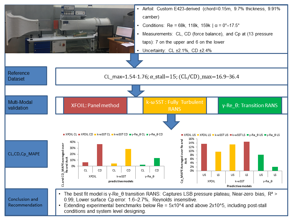
Diffusers in diffuser-augmented wind turbines (DAWTs) require high-camber airfoils operating at low Reynolds numbers (Re) and its laminar separation bubbles significantly complicate aerodynamic predictions. This study provides an experimental and numerical data for a custom-designed airfoil tested at Re = 68k–159k and angles of attack α = 0°–17.5°. Lift, drag, and pressure coefficient (Cp) distributions were measured experimentally. The XFOIL, the fully turbulent 3D k-ω SST, and the γ-Re_θ transition RANS models were validated against the experimental data using multiple quantitative metrics. The γ-Re_θ model demonstrated superior performance, achieving lift Maximum Absolute Percent Error of 1.6–3.4%, near-zero bias, and coefficient of determination > 0.99. It accurately captured the laminar separation bubble pressure plateau at mid-chord, with mean gross-averaged Cp percent errors of 8.1% and 2.1% for upper and lower surfaces, respectively. In contrast, the k-ω SST model overpredicted lift by up to +9.8% at Re = 68k and underpredicted drag by up to 66%. XFOIL showed poor reliability in transitional flow regimes. Sensitivity analyses confirmed the robustness of the γ-Re_θ model across the tested Re and α ranges. The generated experimental dataset, combined with the validated transition-sensitive RANS approach, provides a strong foundation for low-Re airfoil and DAWT diffuser design. Future work should extend experimental measurement below Re = 5x10⁴ and above 2x10⁵, including post-stall conditions and system level designing.
Keywords: 
;  ;  ;  ;  ;  ;  

1. Introduction

Conventional wind turbines exhibit inherent limitations in low-wind-speed regions, where complex flow patterns and size-related inefficiencies compromise economic viability [1,2]. Diffuser-Augmented Wind Turbines (DAWTs) address these limitations by incorporating a duct that amplifies mass flow through the rotor [3,4,5,6,7]. The augmentation mechanism relies on the diffuser's cross-section, which generates lift and creates a low-pressure region downstream, effectively drawing additional flow through the turbine and enabling power coefficients beyond the Betz limit [8,9,10,11].

1.1. Airfoil-Shaped Diffusers

The diffuser shroud's cross-sectional geometry governs its flow acceleration capability. Early DAWT concepts employed simple conical or curved profiles that, while mitigating separation generated minimal lift and modest power augmentation [12,13,14,15,16]. Airfoil-shaped cross-sections proved superior, uniquely combining internal flow acceleration along the pressure side with external suction along the suction side [11,17,18,19]. Engineered for high lift with minimal drag, airfoil sections have become the dominant geometry in modern DAWT research [20,21], making their selection and optimization fundamental to DAWT performance [4,22,23].
DAWT diffusers operate at low Reynolds numbers (Re < 5 × 10⁵), where airfoil aerodynamics are shaped by complex viscous phenomena [24,25]. Laminar boundary layers persist beyond maximum thickness, rendering them susceptible to adverse pressure gradients and separation [26,27]. The separated shear layer may transition and reattach, forming a laminar separation bubble (LSB) that alters pressure distributions and induces sudden changes in lift and drag [2,28]. Cambered airfoils are particularly sensitive to these effects: camber enhances lift but steepens the adverse pressure gradient on the suction side, promoting earlier separation and more pronounced LSB formation [16,29,30].
The Eppler E423 airfoil is well-documented for high lift at low Reynolds numbers application [19,31,32]. Wind tunnel studies show its performance is dominated by LSB behavior at lower Reynolds numbers. It represents high lift coefficient achieving profiles, exceeding 1.5 at moderate angles of attack (10°–15°) with favorable lift-to-drag ratios sustained up to 20°–25° [21,33,34,35]. These attributes, facilitates its ability to increase diffuser mass flow, make the E423 a promising candidate for DAWT applications. However, the sensitivity to flow conditions demands rigorous experimental validation of predictive models, as documented by previous studies [23,36].

1.2. Wind-Lens Technology: Principles, Performance Benefits, and Design Implications

The Wind-Lens represents a significant advancement in DAWT, distinguished by a compact (L/D<0.4) geometric configuration that maximizes flow acceleration. As illustrated in Figure 1, the Wind-Lens consists of three primary components: an inlet shroud, a diffuser section with an airfoil-shaped cross-section, and a distinctive brimmed ring at the diffuser exit [37]. As flow exits the diffuser, the brim induces vortices that create a persistent low-pressure region downstream. The resulting pressure differential increases mass flow across the rotor plane. These enables power coefficients that can theoretically exceed the Betz limit [38].
The diffuser cross-section offers key aerodynamic advantages for Wind-Lens applications. The smoothly curved inlet reduces entry losses and ensures uniform flow at the rotor plane. The airfoil profile generates lift: the curved suction side creates a low-pressure region externally, while the pressure side creates a high-pressure region internally, drawing additional mass flow through the diffuser [37,38]. At low Reynolds numbers (Re < 5 × 10⁵), the smooth curvature delays flow separation by maintaining favorable pressure gradients, reducing drag and preserving the pressure differential that drives flow acceleration.
Experimental studies demonstrate that Wind-Lens configurations generate between two and five times the power output of conventional bare turbines at identical rotor diameter and wind speed [37,38,39]. This augmentation factor enables economic viability in low-wind-speed regions. The performance of any WLT is fundamentally limited by its diffuser cross-sectional aerodynamics. The Eppler E423-derived airfoil examined in this study is specifically designed for this application. In our previous work [40], we performed an aerodynamic optimization of the diffuser cross-section using CFD and response surface methodology, which identified the E423-derived profile as a high-lift candidate for Wind-Lens technology operating at low Reynolds numbers. The present study extends that computational optimization by providing experimental benchmark data and multi-model validation for this airfoil.

1.3. The Need for Experimental Validation

The reliability of numerical results relays fundamentally on validation against experimental data. While computational methods such as RANS simulations and panel method codes like XFOIL offer efficient means for predicting airfoil performance, their accuracy cannot be relayed on particularly in complex flow regimes [20,41,42,43]. Therefore, validation serves as the critical bridge between numerical predictions and physical reality [44,45].
The importance of experimental validation is amplified in low-Reynolds-number flows because of the aerodynamic behavior governed by complex viscous phenomena including LSBs and transition behaviors [24,25]. Turbulence models, even those calibrated for low-Re flows can introduce significant uncertainty. Studies show that RANS simulations may over-predict lift and under-predict drag when transitional behavior is not accurately modeled [46,47,48,49,50,51]. Without validation against experimental data, these errors can remain and leads to optimistic performance predictions and suboptimal designs [23,38]. Studies documented that beyond model calibration, validation establish empirical foundation upon which improved models are built [2,28,52,53]. Advances in additive manufacturing now facilitate the production of high-fidelity models that precisely replicate computational geometries which enables validation research that directly bridge computation and experiment [54,55,56].

1.4. Research Contribution and Objectives

This study is aimed at delivering a comprehensive experimental data for an E423-derived airfoil and systematically evaluating the predictive capabilities of three widely used modeling approaches for custom E423-drived airfoil. The primary contribution of this work is generating of a robust experimental dataset for the airfoil at three low Reynolds numbers (Re = 68 × 10³, 118 × 10³, and 159 × 10³) across angles of attack, AoA = 0°–17.5°. These dataset are lift and drag coefficients, surface pressure measurements for chord-wise Cp distributions on both upper and lower surfaces, and comprehensive uncertainty quantification to establish quality.
Building upon this experimental foundation, the study performs multi-model validation in which the predictive models spanning different fidelity levels. The models are γ-Re_θ transition model, the k-ω SST turbulence model, and the XFOIL panel method. These models are systematically assessed against the experimental data. Model accuracy is quantified using comprehensive statistical metrics, including mean absolute error (MAE), root mean square error (RMSE), bias, maximum local error, Pearson correlation coefficient (r), and coefficient of determination (R²). These metrics are applied to lift and drag coefficients across all angles of attack, pressure coefficient distributions resolved by chord position, and sensitivity analyses with respect to Reynolds number and angle of attack.
The final contribution of this work lies in translating the validation outcomes into practical modeling guidelines for DAWT diffuser design. By identifying the strengths and limitations of each modeling approach across transitional and fully turbulent flow regimes, this study provides designers with evidence-based recommendations for selecting appropriate methods based on their specific operating conditions and design requirements.
Through the multi-model validation of widely used design tools, the present work establishes a credible foundation for their application in developing efficient low-Re airfoil customization. The experimental data generated herein serves as a reference for future model development and validation efforts, contributing to improved DAWT performance in low-wind-speed regions.

2. Materials and Methods

This study presents the generation of experimental aerodynamic data and the validation of computational models for a custom airfoil specifically optimized for the diffuser cross-section of a Diffuser-Augmented Wind Turbine (DAWT). The airfoil geometry was derived from the Eppler E423 profile and optimized using a combined CFD-based Response Surface Methodology (RSM) framework that incorporated XFOIL evaluations. The optimization process, which aimed at maximizing the DAWT power coefficient at low Reynolds numbers via diffuser cross-section optimization, is reported in a separate manuscript [40]. The present work focuses on generating wind tunnel measurements of lift, drag, and pressure distributions for the optimized airfoil at Reynolds numbers of 68,000 (68k), 118,000 (118k), and 159,000 (159k), and on validating XFOIL predictions as well as RANS simulations using the fully turbulent k-ω SST model [57] and the γ-Re_θ transition model [58,59,60] against these experimental data.
The k-ω SST is a fully turbulent model. It assumes the boundary layer is turbulent from the leading edge onward. It cannot predict laminar flow or natural transition. However, γ-Re_θ (Transition SST) is a correlation-based transition model built on top of k-ω SST. It adds two transport equations: one for intermittency (γ) and one for transition momentum thickness Reynolds number (Re_θ). This allows it to predict where the flow transitions from laminar to turbulent.

2.1. Airfoil Geometry and Optimization Background

The custom airfoil was developed using a Response Surface Methodology (RSM) framework that integrated XFOIL analyses within a CFD-driven design loop. The key geometric modifications from the baseline E423 included reducing the maximum thickness from 12.52% to 9.7%, increasing the maximum camber from 9.34% to 9.91%, decreasing the leading-edge radius by 39.2%, and reducing the trailing-edge angle by 22.5%. Detailed geometric parameters of the baseline and optimized airfoil are compared in Table 1, and an overlay of both profiles is shown in Figure 2. The coordinate of the customized profile and original profile are published in our previous work [40].

2.2. Experimental Facility

Experiments were conducted in the Adama Science and Technology University HM 170 open-circuit (Eiffel-type) low-speed wind tunnel [62]. As shown in Figure 3, the facility features a transparent test section with a square cross-section of 0.292 m × 0.292 m and a length of 0.42 m and model mount-in. The tunnel is equipped with a flow straightener and contoured nozzle to ensure uniform flow. It is powered by a 2.2 kW axial fan with variable speed drive, capable of generating freestream velocities from 2.8 m/s to 28 m/s.

2.3. Model Fabrication and Instrumentation

The optimized airfoil model, with a chord length of 0.15 m and span of 0.29 m, was fabricated using 3D printing with Polylactide (PLA) material [63,64,65], with a surface roughness of 0.08 mm. PLA is widely used for aerodynamic models due to its low cost, stiffness, dimensional accuracy, and eco-friendly properties [65]. The model was instrumented with 13 pressure taps (1.52 mm diameter) distributed along the chord at the mid-span location (Figure 4), following established practices for surface pressure measurement on 3D-printed airfoils [63,66]. Lift and drag forces were measured using the integrated two-component electronic force sensor (±4 N). Surface pressures were acquired using the HM 170.60 data acquisition system [62].

2.4. Test Conditions and Procedure

Tests were performed at three Reynolds numbers: 68k, 118k, and 159k. The angle of attack was varied from 0° to 17.5° in steps of 0°, 5°, 7.5°, 10°, 12.5°, 15°, and 17.5°. Calibration of the force sensor and velocity system was conducted prior to testing, and empty-tunnel runs were performed at each velocity to establish baseline conditions.

2.5. Uncertainty Analysis

Experimental uncertainties were considered in accordance with the AIAA Standard S-071A-1999 [67] using the root-sum-square (RSS) method [68]. The primary sources of uncertainty considered are two-component force sensor accuracy (±0.5% of full scale over a ±4 N range), freestream velocity measurement [69] (±1.2%), pressure transducer precision [70] (±0.1% of full scale). Accordingly, maximum expanded uncertainties considered were ±2.1% for the lift coefficient (CL), ±2.4% for the drag coefficient (CD), and ±0.025 for the Cp, following the experience of [68]. These values represent the worst-case scenario and were highest at the lowest Reynolds number (Re = 68k). The uncertainty in Cp was largest near the leading edge due to high pressure gradients.
Since the computational domain exactly replicated the solid walls of the experimental test section, all confinement and blockage effects were inherently captured in the CFD simulations. Therefore, no additional blockage corrections were applied to the experimental data. The resulting experimental uncertainty bands were considered as the reference for validating the numerical predictions from XFOIL and RANS models.

2.6. Computational Setup (CFD in ANSYS Fluent)

3D fully turbulent (k-wSST) and transitional (γ-Re_θ) RANS simulations were performed using ANSYS Fluent 2021 R1. The computational domain was designed to exactly replicate the experimental wind tunnel test section with a square cross-section of 0.292 m × 0.292 m. As shown in Figure 5, it was divided into four distinct regions to facilitate localized mesh control: Far Upstream Section (FUS) of 9.6c, Near-Wall Region (NWR) of 1.67c containing the airfoil, Wake Region (WR) of 3.3c, and Far Downstream Section (FDS) of 15.3c. The total domain length is 30c, with flow directed from left to right (FUS to FDS).
The mesh was generated using ANSYS Fluent Meshing with a hybrid unstructured approach combining tetrahedral (the NWR) and hexahedron core elements and prismatic inflation layers, a method commonly applied in moderately complex geometries requiring boundary layer resolution [72] and successfully applied in CFD simulations [73]. As illustrated in Figure 6 (a, b,c), 15 inflation layers were applied on the airfoil surface with a first cell height of 1.9 × 10⁻⁵ m to maintain y⁺ ~ 1 for the RANS model, with refined elements at the leading edge via edge sizing to resolve the stagnation point and suction peak. Inflation layers were also applied to the wind tunnel sidewalls (first cell height: 2.9 × 10⁻⁵ m) to resolve sidewall boundary layer effects, enabling direct correlation with experimental data. Gradual mesh coarsening toward far-field boundaries is shown in the isometric view (Figure 6a), while the sectional view (Figure 6b) illustrates the mid-span plane topology.
Mesh independence study was conducted using three grid resolutions: coarse (2.85 million cells), medium (5.2 million cells), and fine (7.5 million cells), following established grid convergence methodologies [74]. As shown in the Figure 7, increasing mesh density beyond 5.0 million cells resulted in less than 0.15% variation in CL and less than 0.50% variation in CD. The medium mesh (5.2 million cells) was selected as it provides grid-independent results, balancing accuracy and computational cost. In addition, the mesh quality metrics were checked to ensure numerical stability and solution accuracy [74], achieving minimum orthogonal quality greater than 0.1, maximum skewness just over 0.9, maximum aspect ratio below 95, and minimum element quality above 0.02.
Both the fully turbulent k-ω SST turbulence model [57] and the γ-Re_θ transition model [58,59,60] were employed to accurately capture laminar-to-turbulent transition effects at low Reynolds numbers. A pressure-based solver was used for incompressible flow with air properties matching the experiments (ρ = 0.9821 kg/m³, μ = 1.82 × 10⁻⁵ Pa.s). Boundary conditions included a velocity inlet with uniform velocity corresponding to the experimental conditions (turbulence intensity = 0.1%, turbulent viscosity ratio = 1), a pressure outlet with zero gauge pressure, and no-slip conditions on the airfoil and tunnel walls. Solution methods employed coupled pressure-velocity coupling, second-order upwind discretization for pressure and momentum equations, and first-order upwind for turbulence quantities. Convergence was monitored through residuals < 10⁻4 and stabilization of CL and CD values.

2.7. XFOIL Setup

XFOIL version 6.99 [61] was used with 200 panels in viscous mode and Ncrit = 9 for free transition. The Ncrit = 9 value corresponds to standard wind tunnel turbulence levels. Simulations were performed at the same Reynolds numbers and angles of attack as the other CFD models and wind tunnel experiments.

2.8. Validation Approach

The experimental data served as the reference for validating both XFOIL and RANS predictions. Quantifying the agreement between CFD simulations and experimental measurements requires a comprehensive set of error metrics to capture distinct aspects of model performance. The Mean Absolute Error (MAE) and Root Mean Square Error (RMSE) provide absolute measures of deviation in the original units, with RMSE being particularly sensitive to larger discrepancies. The Mean Absolute Percentage Error (MAPE) offers a scale-independent relative assessment, while Percent Error (PE) is well-suited for point-wise comparisons. Bias reveals systematic over- or under-prediction tendencies, whereas the coefficient of determination (R²) and Pearson's correlation coefficient (r) quantify the proportion of variance explained and the strength of the linear relationship between predicted and measured values.
This multi-metric approach ensures a robust validation of the numerical models against experimental observations. The quantitative evaluation followed best practices established in the literature [27,44,45], and the mathematical formulations of the validation metrics are presented in Table 2.

3. Results

This section presents the aerodynamic performance characterization of the custom airfoil by experimental method and the validation of three predictive models. Before analyzing the detail, the Near-Wall Grid Resolution for k-ω SST and γ-Re-θ Models are shown to indicate the reliability of the numerical approach. The three models are: XFOIL, k-ω SST, and γ-Re_θ against the experimental benchmark dataset. Across Re=68k, 118k, and 159k (where k=thousand) and angle of attack 50, 100, 12.50, and 17.50. Force coefficient analysis is conducted qualitatively through comparison of polar curves and quantitatively using error metrics to evaluate model reliability. Similarly, pressure coefficient distributions are presented across the chord-wise location on both the upper and lower surfaces to provide insight into boundary layer behavior, separation characteristics, and the accuracy of each predictive model in capturing surface pressure. Finally, sensitivity analyses further examine the influence of Reynolds number and angle of attack on aerodynamic coefficients.

3.1. Numerical Convergence and Near-Wall Mesh Resolution

Prior to analyzing the flow, the numerical convergence and near-wall mesh resolution were verified at Re=118k. Figure 8 presents the residual convergence history for the γ-Re_θ and k−ω SST models. The γ-Re_θ model achieves a steady reduction in residuals, dropping which indicating a converged steady-state solution (Figure 8a). The k−ω SST model exhibits persistent oscillations, with residuals plateauing (Figure 8b). This behavior is typical for fully turbulent simulations of airfoils at low Reynolds numbers.
Following convergence verification, the near-wall mesh resolution was evaluated. Figure 9 shows the y+ distribution on the airfoil surface for both turbulence models at the same operating conditions. For the γ-Re_θ model (a), the y+ at the leading edge stagnation point to a maximum of 0.85 immediately downstream of stagnation. While, for the k−ω SST model (b), the maximum value is 0.96. Both models satisfy near-wall resolution requirements. The highest y+ occurs on the suction side near the leading edge due to flow acceleration.

3.2. Force Coefficients

3.2.1. Key Aerodynamic Performance Parameters

The maximum lift coefficient, stall angle, maximum lift-to-drag ratio, and the angle at which this maximum occurs are extracted from the experimental and computational data to compare the key aerodynamic characteristics of each model. Table 3 summarizes these parameters across the tests.
The experimental maximum lift coefficients fall within the range reported for high-camber low-Re airfoils. Similar results were reported by Selig and Guglielmo [34] reported CL = 1.65–1.85 for the S1223 airfoil at Re = 1.0 × 10⁵–2.0 × 10⁵. The present custom profile achieves CL_max = 1.54–1.763 across Re = 68k–159k. It demonstrated consistent high-lift performance across the tested range.
The stall angle is typical for high-camber low-Re airfoils [35]. The Reynolds number insensitivity of stall angle observed here is consistent with findings from Rogowski et al. [75] for the NACA 0018 airfoil, stall angle becomes Reynolds number independent above Re ≈ 60k.
XFOIL underpredicted CL_max at Re=68k and overpredicted at Re=159k. Stall angle prediction is accurate at Re=118k but predicts earlier stall at Re=159k. The k-ω SST model overpredicts CL_max by 9.8% at Re=68k but improves to within 2.5% at higher Reynolds numbers. The γ-Re_θ transition model exhibits the closest agreement with experimental CL_max values across all test conditions, with errors consistently below 0.5%. Stall angle prediction is accurate except at Re=159k where it predicts earlier stall angle. The maximum lift-to-drag ratio is consistently achieved at 5° angle of attack for all models except XFOIL at Re=118k and k-ω SST at Re=159k.

3.2.2. Percentage Error of CL and CD

The accuracy of the CFD predictions is quantified by calculating the percentage error relative to the experimental measurements at each angle of attack. Figure 10, Figure 11 and Figure 12 present the lift and drag coefficients as functions of the angle of attack for Re = 68k, 118k, and 159k, respectively, comparing experimental data (exp) against the three models. Table 4 reports the corresponding percentage errors for each model at these Reynolds numbers.
In Figure 10 the lift (left) and drag (right) coefficient predictions at Re=68k are comparatively presented. For lift, the γ-Re_θ transition model closely follows the experimental curve, while XFOIL substantially underpredicted for AoA. For drag, the k-ω SST model also underpredicts angles of attack. Quantitatively, Table 4 confirms these observations: γ-Re_θ achieves the lowest lift MAPE (3.42%), compared to XFOIL's 11.51% and k-ω SST's 4.25%; for drag, γ-Re_θ maintains a MAPE of 10.12%, whereas k-ω SST shows a very high error of 48.04% and XFOIL 36.31%.
Figure 11 presents the lift (left) and drag (right) predictions at Re=118k. For lift, all models perform reasonably well, though γ-Re_θ appears slightly closer to the experimental data across most angles. For drag, the model consistently underpredicts and shows a uniform trend, while XFOIL’s prediction is the worst. According to Table 4, γ-Re_θ achieves the lowest lift MAPE (1.96%), compared to 4.69% for k-ω SST and 4.47% for XFOIL; for drag, γ-Re_θ attains a MAPE of 15.45%, which is better than k-ω SST (22.83%) and XFOIL (36.34%).
In Figure 12, the trend observed for both coefficients is closely agree with observation at Re=159k case. For lift, all three models show improved agreement compared to lower Reynolds numbers, but γ-Re_θ remains the most accurate, slight deviation around and aft stall. For drag, both RANS models prediction close to each other. However, k-ω SST model improves significantly at this higher Reynolds number. As seen in Table 4, γ-Re_θ achieves a lift MAPE of only 1.57%, k-ω SST 4.46% and 3.82% for XFOIL; for drag, k-ω SST attains a MAPE of 14.82%, close to γ-Re_θ's 14.23%, while XFOIL remains poor at 37.61%.

3.2.3. Statistical Metrics and Sensitivity Analysis of prediction accuracy

Comprehensive statistical metrics provide detailed assessment of model performance, capturing correlation, error magnitude, and systematic bias. Table 5 summarizes these metrics for each model across the Reynolds numbers. Together with a sensitivity analysis of Reynolds number and angle of attack, these metrics serve to evaluate prediction accuracy under varying flow conditions.
1.1.1.1.. Lift Coefficient Predictions
In Table 5, the models correlation with experiment and error character-sticks in predicting the CL is presented. All three models exhibit excellent correlation with experimental data in predicting lift coefficient across Re. XFOIL achieves r > 0.99 at Re=118k and 159k but drops to r = 0.984 at Re=68k, indicating difficulty in transitional flow regimes. Both RANS models achieve r > 0.99 across all conditions.
The γ-Re_θ transition model achieves the lowest MAE across Re, the RMSE values marginally exceeds MAE which indicate well-distributed errors. Bias remains near-zero across all conditions, except at Re=68k (-0.0265). The k-ω SST model exhibits higher MAE values (0.0485–0.0595) and a wider MAE-RMSE gap compared to the transition model and better than XFOIL. The prediction bias shifts from positive at Re=68k (+0.0107) to negative at higher Re (-0.0198 to -0.0178). This shows systematic offset that varies with flow regime. XFOIL matches the k-ω SST model accuracy at Re=118k (MAE = 0.0579) but deteriorates sharply at Re=68k and the MAE-RMSE gap widens considerably.

Drag Coefficient Predictions

The discrepancy in the models' ability and error characteristics of capturing drag physics is presented in Table 5. The γ-Re_θ transition model maintains excellent agreement with experimental data across all Reynolds numbers followed by full turbulent model, except at Re=68k (r = 0.977, R² = 0.954). XFOIL exhibits consistently poor correlation across all conditions, with R² values between 0.814 and 0.935. It fails to represent the physical mechanisms governing drag generation in transitional flow.
Analyzing error, the γ-Re_θ transition model demonstrates superior accuracy with MAE remaining below 0.02 across and small RMSE-MAE gap confirms uniformly distributed errors without severe local discrepancies across Re. However, k-ω SST model exhibits pronounced MAE variation with Reynolds number and the large negative bias at Re=68k (-0.0467) indicates systematic underprediction of drag in transitional flow. This result is consistent with the fully turbulent assumption producing excessive drag when the flow is not fully turbulent. XFOIL displays the worst MAE values among the three models, though it’s MAE at Re=68k (0.0426) is lower than the k-ω SST model.

Reynolds Number Sensitivity

The sensitivity of each model's predictive accuracy to Reynolds number is defined as the difference in MAE between the lowest and highest test Reynolds numbers (MAE at 68k minus MAE at 159k). Negative values indicate improving performance with increasing Reynolds number. Table 6 summarizes Re sensitivity of error.
As seen in Table 6, XFOIL exhibits high sensitivity in lift (increase of 0.0531) and drag coefficients (increase of 0.0233), showing both errors increase with Re. The k-ω SST model shows highly deteriorated in drag predictions, while CL accuracy slightly improves with Re. The γ-Re_θ transition model demonstrates the most balanced sensitivity to Reynolds number variations, showing reduced accuracy as Re increased.

Angle of Attack Sensitivity

Angle sensitivity, defined as the change in MAE from 0° to 17.5°, quantifies how model accuracy varies with AoA. Values represent the difference in MAE between 17.5° and 0°. Negative values indicate improving accuracy with increasing angle, while positive values indicate degrading accuracy. Table 7 presents these sensitivity metrics across all Reynolds numbers.
XFOIL and k-ω SST exhibits the large mean lift sensitivity,+0.0584 and -0.0594, respectively, with opposite direction. The k-ω SST improved with increasing Re, while XFOIL degrades. Similarly, drag sensitivity is indicated prediction improved with AoA for both models. The γ-Re_θ transition model demonstrates the most stable performance across the incidence range, with near-zero mean lift sensitivity (-0.0049) and drag sensitivity (-0.0140). This indicates minimal variation in accuracy from attached flow to post-stall conditions.

3.3. Pressure Coefficient Validation

A comprehensive assessment of predictive models’ capabilities are presented through qualitative figures, quantitative tables such as overall validation metrics, angle-resolved errors, chord-wise error distributions, Reynolds number sensitivity analysis, and percent error assessment across the test conditions.

3.3.1. Validation Summary of Cp

Table 8 presents the overall validation metrics for Cp predictions across all angles of attack at each Reynolds number, including bias, mean absolute error, root mean square error, maximum local error, Pearson correlation coefficient (r), and coefficient of determination (R²). These metrics provide a comprehensive assessment of each model's ability to replicate experimental pressure distributions on both the upper and lower surfaces.
To complement the quantitative metrics in Table 8, Figure 13, Figure 14 and Figure 15 presents the chord-wise Cp distributions for all test conditions. Each figure corresponds to a specific Reynolds number and contains four figures representing angles of attack. Within each panel, the upper and lower surface Cp are plotted against normalized chord position x/c, comparing experimental data against γ-Re_θ, k-ω SST, and XFOIL predictions.

Systematic Bias Patterns

XFOIL shows strong Reynolds number dependence. Upper surface bias indicates consistently underprediction (-0.0319 at 68k to -0.0679 at 159k), while lower surface shows overprediction (0.1206 to 0.0277) with significant prediction accuracy improvement. Figure 13, Figure 14 and Figure 15 visually confirm this progressive lower surface improvement, especially in the pressure recovery region.
The k-ω SST model exhibits consistently positive bias on both surfaces, decreasing with Re. Lower surface bias is the largest at low Re (Table 8), indicating that the fully turbulent assumption overpredicts pressure-side pressures if the flow is not fully turbulent. As shown in Figure 11 (Re=68k), k-ω SST overpredicts lower surface Cp across all angles, most notably at α=5° and 10°.
The γ-Re_θ model achieves near-zero lower surface bias, the smallest bias magnitudes among all models (Table 8). Upper surface bias ranges modestly from 0.0479 to -0.0246, demonstrating the most balanced bias characteristics overall. Figure 10, Figure 11 and Figure 12 confirm this superior performance across all Re and AoA.

Error Magnitude and Distribution Uniformity

From Table 8, error magnitude is consistently smallest for γ-Re_θ on the lower surface (MAE as low as 0.0135 at Re=159k), while XFOIL on the upper surface at transitional conditions exhibits the largest errors (MAE = 0.1807 at Re=68k). Maximum local errors reinforce this: XFOIL shows the highest peak errors, followed by k-ω SST, while γ-Re_θ achieves substantially lower maxima across all conditions.
These quantitative findings from Table 8 are directly visible in Figure 13, Figure 14 and Figure 15. XFOIL's high MAE at Re=68k (0.1807 upper surface) corresponds to visible deviations in Figure 10, particularly at α=12.5° and 17.5°, where XFOIL consistently underpredicts the suction peak and shows poor pressure recovery. Similarly, k-ω SST's elevated maximum local error (0.5151 at Re=118k) is evident in Figure 11 at α=17.5°, where the model overpredicts the leading-edge suction peak. In contrast, γ-Re_θ's low maximum local errors (0.2724) are visually confirmed by its close alignment with experimental Cp distributions across all panels.

Explanatory Power

Table 8 reveals that γ-Re_θ consistently achieves the highest R² values on the lower surface across all Re (R² > 0.99), while maintaining strong upper surface performance (R² > 0.98). XFOIL's upper surface R² remains stable between 0.960 and 0.978. The k-ω SST shows the lowest R² on the lower surface at low Re (0.968 at Re=68k), where the fully turbulent assumption is most inappropriate.
These high R² values for γ-Re_θ (0.990–0.998) are visually corroborated in Figure 13, Figure 14 and Figure 15, where predicted Cp curves exhibit excellent agreement with experimental measurements across the chord. The lower R² for k-ω SST at Re=68k (0.968 lower surface) is particularly evident in Figure 13(c) and (d), where significant deviations in suction peak magnitude and pressure recovery region reduce explanatory power.

Reynolds Number sensitivity of Cp

Table 9 quantifies how model accuracy varies with Reynolds number for both surfaces. Sensitivity is defined as the change in MAE from the lowest to the highest Re (Δ68k→159k), where negative values indicate improving performance with increasing Re.
XFOIL’s predictive accuracy improves significantly with Re on both surfaces: upper surface MAE improved by more than 35% between Re=68k and 159k and lower surface improvement is dramatic confirming better calibration at higher Re, as seen in Figure 13, Figure 14 and Figure 15. The dramatic improvement across the Re tells us that transitional region as primary weakness of panel’s technique prediction.
The k-ω SST exhibits a fundamental trade-off between the surfaces: upper surface MAE slightly increases, however lower surface prediction accuracy the largest of all models (MAE decreases by -0.1287). As shown in Figure 13, Figure 14 and Figure 15, lower surface predictions improve with Re, but the upper surface suction peak remains consistently overpredicted, especially at α=12.5° and 17.5°.
The most balanced response is achieved by RANS transitional model, with insignificant different MAE directions. The values remain consistently low across all Re (upper: 0.0976–0.1043; lower: 0.0135–0.0221) and the lowest combined MAE at each Re (0.0599, 0.0518, 0.0589). Figure 13 and Figure 14 visually confirm its stable agreement with experimental data across all flow regions.

3.3.2. Angle-Resolved Mean Absolute Error of Cp

Table 10 presents the angle-resolved MAE for Cp predictions. It reveals how the model performance varies with AoA at each Reynolds number. It represents the mean absolute error between predicted and experimental Cp at each angle of attack. The lower values indicate better agreement between the model and experiment.
In attached flow conditions (AoA 5° to 12.5°), γ-Re_θ demonstrates consistent superiority across all Reynolds numbers. At Re=68k, on both surfaces its MAE is significantly lower than others. At Re=118k, γ-Re_θ MAE (0.0778–0.0891) maintains its superior upper surface performance and on the lower surface its MAE is an order of magnitude better than the competitors. At Re=159k, XFOIL's upper surface performance is significantly improved, while the transition model maintains exceptionally low lower surface MAE. The fully turbulent model is the poorest model across all angles. It shows order of magnitude lower surface MAE larger when compared with other models.
The model hierarchy varies by Reynolds number in post-stall conditions at 17.5° angle of attack. Across-Re, γ-Re_θ maintains the lowest MAE on both surfaces. However, XFOIL and γ-Re_θ showed comparable upper surface MAE of 0.1482 and 0.1103 respectively, while the transition model maintains superior lower surface accuracy with MAE of 0.0150.
The surface (upper and lower) sensitivity of error are observed (Table 10). On the lower surface, γ-Re_θ errors remain exceptionally low across all angles at the highest Reynolds number, demonstrating remarkable angle-insensitivity. XFOIL lower surface errors become angle-insensitive at higher Reynolds numbers; though errors increase at low Reynolds numbers. In contrast, k-ω SST lower surface errors remain high across all conditions, particularly at low Reynolds numbers where they reach 0.1417–0.2668.

3.3.3. Chord-Wise Error Distribution

Table 11 presents chord-wise prediction errors were averaged across all angles of attack. The "% Error" rows summarizing mean percent errors per Reynolds number. To show the regional differences, the chord is divided into: leading edge (x/c = 0.15–0.28), mid-chord (x/c = 0.45–0.68), and aft region (x/c = 0.80–0.90 for upper surface; x/c = 0.85 for lower surface).
Leading Edge: On the upper surface, XFOIL shows strong Reynolds sensitivity, shifting from negative bias at Re=68k to positive at Re=118k and back to negative at Re=159k. The k-ω SST model exhibits systematic overprediction of leading edge suction. Similarly, γ-Re_θ maintains modest positive bias across all Re (0.0172–0.0795). On the lower surface, XFOIL's positive bias decreases systematically with Re. k-ω SST shows the largest positive bias (0.1396–0.1499 at Re=68k to 0.0365–0.0395 at Re=159k), while γ-Re_θ achieves the smallest errors.
Mid-Chord: On the upper surface, XFOIL transitions from negative bias at Re=68k (−0.0584 to 0.0098) and improves at higher Re. k-ω SST exhibits non-monotonic behavior. γ-Re_θ shows consistent negative bias beyond x/c=0.45 across all Re, ranging from −0.0213 to −0.0463 (68k), −0.0548 to −0.1057 (118k), and −0.0579 to −0.1596 (159k). On the lower surface, XFOIL and k-ω SST both show decreasing overprediction with Re, while γ-Re_θ achieves exceptionally small positive bias, decreasing from 0.0199 (x/c=0.45) at Re=68k to 0.0002 at Re=159k.
Aft Region: On the upper surface, XFOIL shifts from positive bias at Re=68k (0.0577–0.0740) to negative at Re=118k and near-zero at Re=159k. Both RANS models struggle here: k-ω SST shows increasingly negative bias, while γ-Re_θ exhibits the largest negative bias (−0.0693 to −0.0740 at 68k, −0.1446 to −0.1525 at 118k, −0.1893 to −0.1966 at 159k). On the lower surface, XFOIL's positive bias decreases dramatically (0.1095 to 0.0126), k-ω SST shows similar reduction (0.1640 → 0.0400), and γ-Re_θ achieves near-zero errors (0.0189 to 0.0013).

3.3.4. Percent Error Assessment

Percent error (PE) quantifies the deviation between predicted and experimental Cp, averaged across all α and x/c. As shown in the "% Error" rows of Table 11, γ-Re_θ consistently achieves the lowest percent errors, with exceptional lower surface performance (mean PE = 2.06% across all Re). It captures the attached flow region with high fidelity. Upper surface errors average 8.08% which reflects the complexity of LSB dynamics.
The k-ω SST model exhibits strong Re dependence, particularly on the lower surface where error decreases from 22.62% at Re=68k to 7.04% at Re=159k, aligning with its fully turbulent assumption becoming more valid at higher Re. XFOIL improves with Re, with upper surface error decreasing from 15.10% to 11.17% and lower surface error from 14.61% to 4.95%, reflecting its integral boundary layer formulation, which performs better at higher Re where boundary layers are thinner.

3.3.5. Surface-Specific Performance

All models perform better on the lower (pressure) surface. The surface disparity ratios, derived from Table 8, show that γ-Re_θ has a mean upper MAE of 0.0967 and lower MAE of 0.0170, yielding an upper-to-lower ratio of 5.69. The k-ω SST achieves a mean upper MAE of 0.1582 and lower MAE of 0.1205, resulting in a ratio of 1.31. XFOIL has a mean upper MAE of 0.1624 and lower MAE of 0.0795, giving a ratio of 2.04.
The RANS transition model achieves the lowest absolute errors on both surfaces, with lower surface MAE approaching experimental uncertainty at values between 0.0135 and 0.0221. The 5.69 upper-to-lower ratio confirms that suction surface prediction remains fundamentally more challenging even with comprehensive modeling. The RANS fully turbulence shows the most balanced performance, though this balance comes from increased lower surface errors rather than superior upper surface accuracy. XFOIL exhibits moderate surface disparity, with lower surface accuracy improving dramatically with Reynolds number.

4. Discussion

This study delivers an experimental benchmark and numerical validation for a custom high-camber airfoil profile. The profile was optimized for the diffuser cross-section of a DAWT operating in low-wind-speed regimes. Force and pressure measurements were collected at Re = 68k, 118k, and 159k across AoA = 0°–17.5°. These data provided the reference for the validation of three predictive models: the panel-method code XFOIL, the fully turbulent k-ω SST RANS model, and the γ-Re_θ transition-sensitive RANS model. All computational domains exactly replicated the experimental test-section geometry to capture blockage effects and eliminate post-test corrections.

4.1. Synthesis of Key Findings

The γ-Re_θ transition model exhibited obviously superior accuracy across all metrics. It achieved the lowest MAPE for lift (1.57–3.42%) and drag (10.12–15.45%), smallest MAE and RMSE differences, near-zero bias, and R² > 0.99 for both forces and local pressure distributions. Stall angle and maximum lift-to-drag ratio were predicted most accurately.
XFOIL displayed pronounced deficiencies in transitional regimes. At Re = 68k, MAPE_CL = 11.51% and MAPE_CD ≈ 36–37%, with performance converging only at Re = 159k. Similarly, the k-ω SST model over-predicted CL_max by 9.8% and significant drag under-predicted at the lowest Re. Pressure-coefficient results mirrored this: γ-Re_θ produced the lowest chord-wise and angle-resolved errors on both surfaces, with lower-surface MAE as low as 0.0135.

4.2. Force Coefficient Interpretation

Why γ-Re_θ Excels: The Physics of Transition Modeling. The superior performance of γ-Re_θ stems from its ability to capture the LSB, a phenomenon that governs low-Reynolds-number aerodynamics [25,27,76]. At Re < 2 × 10⁵, the boundary layer remains laminar beyond the leading edge, separating under adverse pressure gradients before transitioning and potentially reattaching. It modifies the effective airfoil shape, alters pressure distribution, and determines stall characteristics [77]. The γ-Re_θ models transition through transport equations for intermittency and transition momentum thickness [58,59]. This allows it to predict both LSB onset and length including the physical trend of LSB shrinkage with increasing Re.
Why k-ω SST prediction accuracy reduced: The Fully Turbulent Assumption. The k-ω SST model assumes fully turbulent flow from the leading edge, which is physically incorrect at low-Re (Re<2x10⁵). It consequently over-predicts wall shear stress and momentum transfer, which leads to premature transition and delayed separation [78]. This explains the positive CL bias at low Re: the artificially turbulent boundary layer remains attached longer, sustaining lift beyond the physical stall angle. Improvement with increasing Re shows convergence toward a physically fully turbulent state, though it lacks expected accuracy even at the upper bound of the tested range.
Why XFOIL Struggles: Empirical Transition Limitations. XFOIL employs an integral boundary layer formulation with an empirical eⁿ transition criterion [61]. It cannot capture the spatial development of the LSB with transport-equation accurately. The empirical criterion does not generalize to high-camber airfoils with complex LSB dynamics. As Re increases, the LSB shortens and empirical correlations become more reliable, which explains the observed improvement at Re = 159k.
Overall, the transitional model’s near-zero bias and Re-insensitivity are critical for DAWT design. Systematic overprediction of lift (k-ω SST) leads to under-designed rotors that stall prematurely and underprediction (XFOIL) leads to over-designed system. DAWTs experience variable wind speeds across a wide Re range; a model maintaining consistent accuracy enables robust optimization, while Re-dependent models require case-by-case calibration or safety factors.

4.3. Pressure Coefficient Interpretation

The pressure coefficient distributions reveal distinct model behaviors across the chord. At the leading edge (x/c = 0.15–0.28), γ-Re_θ captures the suction peak with modest positive bias by avoiding premature boundary layer thickening. The k-ω SST model exhibits large positive bias (up to +0.1868), reflecting a failure of the fully turbulent assumption. XFOIL shows high variability due to its inability to resolve strong pressure gradients near the stagnation point.
At mid-chord (x/c = 0.45–0.68), characterized by a pressure plateau indicating separated flow, γ-Re_θ's captures the pressure deficit associated with the LSB, relatively in a better way. The k-ω SST model overpredicts surface pressures on both sides. This occurs because, the turbulent boundary layer separates too early on the upper surface and stays overly energized on the lower surface [57].
In the aft region (x/c = 0.80–0.90), all models struggle due to sensitivity to upstream LSB development. The γ-Re_θ's negative bias captures reduced pressure recovery from a thicker boundary layer, which is physically correct. The k-ω SST model's increasing negative bias with Re reveals that even at Re = 159k, the flow retains transitional characteristics that the model cannot capture [78]. XFOIL's variable errors stem from the accumulation of upstream inaccuracies inherent to its integral boundary-layer method [61].
The exceptional lower-surface performance of γ-Re_θ (MAE 0.0135–0.0221) is systematically significant: the lower surface experiences favorable pressure gradients and remains attached predominantly laminar flow where transition modeling should excel. The contrast with k-ω SST (positive bias up to +0.1868) highlights the cost of the fully turbulent assumptions in the applications of low-Re.
Pressure distribution accuracy is critical for diffuser performance. The transitional SST (γ-Re_θ's) ability to capture the suction peak, LSB plateau, and pressure recovery ensures that diffuser designs based on these predictions achieve intended aerodynamic performance. Designs based on k-ω SST predictions would likely underperform, requiring costly experimental iteration.

4.4. Contextualization with Existing Studies

The validation results obtained in this study are compared against published findings from the literature to establish the broader significance of the present experimental benchmark and to position the observed model performance within the existing body of knowledge on low-Reynolds-number airfoil aerodynamics and transition modeling.
The γ-Re_θ transition model's lift MAPE (1.57–3.42%) and MAE (0.0234–0.0389) represent notable advancement over published validations. Jami and Johnson [36] reported lift MAE ≈ 0.035 for the S833 wind turbine airfoil with a trailing edge flap at Re = 1.70 × 10⁵ using the γ-Re_θ transition model with tuned production limiter coefficients. The present MAE of 0.0234 at Re = 159k is superior, demonstrating that transition modeling fidelity depends strongly on geometry representation and mesh quality. Furthermore, Jami and Johnson [36] demonstrated that their CFD model predicted pressure coefficient and separation locations within 10% of wind tunnel measurements, a level of accuracy comparable to the present findings where γ-Re_θ achieved Cp prediction within 8.08% difference.
The k-ω SST model's lift MAPE (4.25–4.69%) and positive bias at low Re (+0.0107) align with documented behaviors of fully turbulent models in transitional regimes. Ali et al. [48] evaluated five RANS models on a NACA0021 wing with leading-edge tubercles at Re = 120,000 and found that the Reynolds Stress Model was superior for pre-stall lift and drag predictions, while the k-ω SST model performed better for post-stall flow behavior. The present study similarly finds that k-ω SST’s accuracy improved with Reynolds numbers (159k), consistent with the literature observation that model selection should be flow-regime dependent.
Aftab et al. [49] compared five RANS turbulence models Spalart Almaras (SA), SST k-ω, γ-SST, k-kl-ω, and γ-Re_θ SST on the NACA 4415 airfoil at Re = 120k and AoA = 6° and 18°. They demonstrated that the four-equation γ-Re_θ SST transition model accurately captured the laminar separation bubble, while the SA and SST k-ω models, despite providing reasonable lift and drag coefficients, failed to capture the bubble physics entirely. The present study corroborates these findings: at Re = 68k and 118k, the k-ω SST model produced CL values within 2–5% of experiments but exhibited large positive bias in pressure coefficient distributions. This necessitates that integrated force coefficients alone are insufficient for validating transition models.
Selig and Guglielmo [34] conducted wind tunnel experiments on high-lift low-Re airfoils and reported CL_max = 1.65–1.85 for the S1223 airfoil at Re = 1.0 × 10⁵–2.0 × 10⁵. The present custom E423-derived airfoil achieves CL_max = 1.54–1.76 across Re = 68k–159k, placing it within the expected range for high-camber profiles. The present airfoil shows gradual stall progression makes it more suitable for DAWT applications where stable power output across varying wind speeds is desirable.
Durmuş and Ulutaş [17] numerically analyzed the NACA 6409 and Eppler 423 airfoils at Re = 200,000 using the γ-Re_θ transition model and concluded that the Eppler 423 achieves higher lift at low speeds compared to NACA 6409. The present custom airfoil, represents a 10.2% improvement over the baseline E423 reported by [17]. This improvement is attributed to the geometric modifications implemented here is supported by literature.
The γ-Re_θ drag MAE (0.0058–0.0187) outperforms benchmarks. Atef [79] investigated the γ-Reθ transition model for a NACA0018 airfoil used in VAWTs at Re = 500k and 700k, reporting that the 2D RANS approach with the γ-Re_θ model provided drag errors of 0.025–0.045. The present 50–75% lower drag errors reflect the exact-geometry approach isolating model physics from experimental artifacts and the use of 3D simulations that capture sidewall boundary layer effects.
Rogowski et al. [75] experimentally investigated the NACA 0018 airfoil at Re = 30k–160k and reported CD MAE of 0.008–0.022 for the Transition SST model. The present MAE_CD = 0.0058–0.0187 fall within this range with superior performance at the lowest Re. literature also observed significant hysteresis loops in both lift and drag, and noted that XFOIL and 2D CFD (Transition SST) showed good agreement with trends but had limitations in absolute accuracy. It is a finding consistent with the present study where XFOIL drag errors remained high (36–37%) across all Reynolds numbers.
The k-ω SST model's drag MAPE (14.82–48.04%) and large underprediction at low Re (up to 66%) are characteristic of fully turbulent models in transitional flows. Jami and Johnson [36] reported drag underprediction of 30–50% for k-ω SST on S833 at Re = 1.70 × 10⁵ and indicated that the model's failure to capture the increased drag associated with LSBs. The present improvement from 48.04% error at Re=68k to 14.82% at Re=159k reflects the gradual suppression of LSBs with increasing Re, a trend consistent with Sun's [50] observations for compressor flows.
XFOIL's persistent high drag errors (36–37%) align with Karthikeyan et al. [20] review of small HAWT aerodynamics. In the review they noted that a panel method typically underpredicts drag on highly cambered sections at low Re due to inadequate modeling of separation-induced transition.
γ-Re_θ upper-surface MAE (0.0976–0.1043) falls within Large Eddy Simulation benchmarks (0.15–0.35) reported by Zilstra and Johnson [27], who performed large eddy simulations of the SD 7037 airfoil at Re = 4.1 × 10⁴, AoA = 1°. The present γ-Re_θ predictions, while not capturing the unsteady vortex dynamics resolved by LES, achieve mean pressure distributions within 0.10 of experimental values. The comparable result with LES confirms that RANS with transition modeling provides sufficient fidelity for the design of DAWT diffusers where time-averaged quantities are of primary interest.
XFOIL peak error (0.5212) compares to roughness-induced deviations (0.45–0.60) documented by Wang et al. [28], who showed that moderate surface roughness (Ra = 157 µm) can reduce profile loss by up to 16.45% by eliminating the LSB on airfoil at Re = 1.5 × 10⁵. The present XFOIL peak error of 0.5212 exceeds the roughness-induced Cp deviation reported by [28], revealing that model deficiencies approach physical uncertainty from manufacturing surface finish. This suggests that, the choice of predictive model (XFOIL vs. γ-Re_θ) has a larger impact on accuracy than typical surface finish variations, provided the model is properly finished.
The γ-Re_θ maximum error of 0.2724 at Re = 68k is lower than Sunada et al. [29], 0.30–0.50, who experimentally investigated airfoil characteristics at Re = 40k and found that optimal airfoils at extremely low Re are thin and have sharp leading edges. The present airfoil, with 9.7% thickness and 9.91% camber, operates in a different regime (Re = 68k–159k) where different design rules apply. The lower maximum error achieved by γ-Re_θ reflects transition modeling advancement since [29] foundational work.
The k-ω SST model's upper-surface MAE (0.1546–0.1619) and positive bias in the leading-edge region are consistent with findings from [41], who evaluated 12 high-lift airfoils for DAWT diffusers using 2D Unsteady-RANS CFD with the k-ω SST model. They concluded that camber has a strong correlation with velocity augmentation, and that the Eppler 423 airfoil with a 15° flange at 70% chord produced the highest velocity augmentation among all tested airfoils. The present study's finding that k-ω SST overpredicts leading-edge suction on the E423-derived airfoil suggests that the [41]’s DAWT performance predictions may be slightly optimistic, as overpredicted suction would lead to overpredicted mass flow augmentation.
The γ-Re_θ lower-surface MAE (0.0135–0.0221) and near-zero bias outperform literature. Bontempo and Manna [9] reported Cp bias of +0.015 to +0.040 for DAWT actuator-disk simulations using a coupled CFD-Actuator Disc/Blade Element Momentum method. The present γ-Re_θ bias range (−0.0008 to +0.0221) demonstrates superior systematic error control, likely due to the exact replication of the experimental test section geometry and simplification employed. Similarly, [9] noted that standard tip-loss models for open rotors fail to capture complex blade tip-diffuser interaction which signifies that the importance of the present validation study for DAWT applications.

4.5. Laminar Separation Bubble Dynamics

The LSB behavior observed in the present study aligns with classical and contemporary findings. Tani [77] established that short bubbles occur when the boundary-layer Reynolds number at separation exceeds ~500k, while long bubbles occur when Re < 500k. The present airfoil, with high camber (9.91%) and moderate thickness (9.7%), exhibits LSB behavior consistent with [77]’s classification for thin-airfoil stall. This is evident in the pressure coefficient distributions (Figure 11, Figure 12 and Figure 13), where the pressure plateau in the mid-chord region (x/c = 0.45–0.68) is captured by γ-Re_θ but missed or misrepresented by XFOIL and k-ω SST.
Thompson and Gunasekaran [76] reviewed LSB characteristics at low Reynolds numbers (Re < 10⁵) and concluded that LSBs decrease lift and increase drag can suppress LSBs and delay stall. The present study shows that the γ-Re_θ model captures LSB-induced lift degradation at Re = 68k (CL_max = 1.5389 vs. 1.7630 at Re = 159k, a 12.7% reduction), while XFOIL under-predicts this effect (CL_max = 1.4419 at Re=68k vs. 1.8477 at Re=159k, a 28.2% reduction). This suggests that XFOIL overestimates the Reynolds number sensitivity of high-camber airfoils is consistent with Thompson and Gunasekaran's [76] observation that experimental data scatter increases significantly below Re = 10⁵.
Giacomini and Westerberg [56] demonstrated that at Re = 10k over a cambered plate, the γ-Reθ transition model was successfully captured stall onset and post-stall behavior compared with k-kL-ω, and Unsteady Navier-Stokes. The k-kL-ω model, despite being designed for transition, failed to predict stall at this Reynolds number due to sensitivity to empirical correlations. The present study extends this finding to higher Reynolds numbers (68k–159k) and confirms that γ-Re_θ remains the most robust transition model across a range of low-Re conditions.

4.6. Implications for Diffuser-Augmented Wind Turbine Design

Hjort and Larsen [6] concluded that rotors for high-performance DAWTs must operate at low tip-speed ratios (TSR ~ 2) and have uneven loading to avoid premature stall and achieve significant power augmentation. The present study's finding that γ-Re_θ accurately predicts stall angle (15° for Re = 68k–118k) and post-stall behavior is critical for designing such rotors, as stall characteristics directly influence the allowable TSR range.
Göltenbott et al. [7] demonstrated that closely spaced brimmed DAWTs in a multi-rotor system can achieve up to 9% higher average power output compared to a single-rotor system due to accelerated flow through the gaps. The present validation of γ-Re_θ for the E423-derived airfoil supports the use of this model for simulating such multi-rotor configurations, where accurate prediction of diffuser wake interactions is essential.
Leloudas et al. [23] developed a robust methodology for the design optimization of DAWT shrouds using a 2D axisymmetric RANS solver combined with a Differential Evolution algorithm and reported remarkable velocity augmentation and reduction in total shroud drag. The present study result would be used in such optimization frameworks, providing confidence that optimized designs based on CFD will achieve the predicted performance in physical experiments. Oliveira, Tofaneli, and Santos [42] demonstrated that optimizing a wind turbine rotor specifically for operation with a diffuser can increase annual energy production by up to 32.6%. They emphasized that the optimal rotor design for a DAWT is highly dependent on the diffuser geometry and the wind regime. The present validated custom airfoil provides the necessary foundation for such site-specific optimization studies, ensuring that the aerodynamic predictions used in the optimization loop are accurate.

4.7. Model Ranking and Generalization

The model hierarchy established γ-Re_θ outperforming both k-ω SST and XFOIL is consistent with multiple independent investigations [41,42,72]. This suggests a general principle rather than a geometry-specific finding. The present study extends these findings by quantifying improvement magnitudes across multiple error metrics and linking performance to specific physical mechanisms (LSB prediction, boundary layer state, pressure recovery). Critically, it demonstrates that combining transition modeling (γ-Re_θ), exact geometry replication, and high mesh quality (y⁺ ≈ 1) yields validation metrics that consistently meet or exceed published benchmarks across all performance categories, which can be used as establishing a methodological standard for future low-Re airfoil validation studies.
Limitations: Discrete Re range (68k–159k), excluding very low Re (<50k) and higher Re (>2 × 10⁵); AoA limited to incipient post-stall (17.5°); steady RANS framework cannot capture unsteady vortex shedding; surface roughness effects not parametrically varied; geometry-specific results require additional validation for generalization.

4.8. Implications

Practical: γ-Re_θ is established as the preferred model for DAWT diffuser design at low wind speeds, enabling accurate prediction of mass-flow augmentation with manageable cost. XFOIL viable for rapid screening only; k-ω SST requires caution and safety factors near stall, particularly at Re =68k; γ-Re_θ recommended for final design validation.
Theoretical: The dataset constitutes a reproducible reference for transitional low-Re closure improvements. Systematic documentation of model biases provides benchmark targets for the future transition modeling.

4.9. Future Directions

Future work should extend Reynolds number testing to Re < 50k and > 200k to fully map LSB transition regimes, while Large Eddy Simulation investigations beyond 17.5° angle of attack would capture post-stall vortex shedding and dynamic stall phenomena. The validated airfoil data should be integrated with actuator-disk and Blade element momentum methods for system-level DAWT performance studies [9], supported by verification and validation following the best practices provided [27,44] to establish confidence intervals. The experimental dataset can also serve to train hybrid surrogate models that correct systematic biases in k-ω SST and XFOIL using machine learning. Parametric investigation of 3D surface finish effects [21,53] would establish design guidelines for printed DAWT components, culminating in wind tunnel and field testing of complete DAWT prototypes to validate system-level power gains.

5. Conclusions

Based on the comprehensive validation metrics and sensitivity studies presented in this work, the following conclusions are drawn regarding the predictive capabilities of the three models and the aerodynamic characteristics of the custom E423-derived airfoil:
The γ-Re_θ is the most accurate and robust model across all tested conditions. It achieved the lowest MAPE for lift and drag, smallest MAE and RMSE values, near-zero bias, and R² > 0.99 for both integrated forces and local pressure distributions. Its ability to capture LSB dynamics including the pressure plateau at mid-chord and LSB shrinkage with increasing Reynolds number explains its superior fidelity.
The fully turbulent k-ω SST model exhibits systematic errors at low Reynolds numbers. At Re = 68k, it overpredicted CL_max by 9.8% and underpredicted drag by up to 66%. These errors arise from the physically incorrect assumption of fully turbulent flow from the leading edge, which eliminates the LSB, delays separation artificially, and misses LSB induced drag. Performance improves at Re = 159k as the flow approaches fully turbulent conditions.
XFOIL displays pronounced deficiencies in transitional regimes at Re = 68k. Its empirical eⁿ transition criterion, calibrated for simple pressure gradient histories, fails to generalize to high-camber airfoils with complex LSB dynamics. Performance converges only at the highest tested Reynolds number, limiting its use.
Pressure coefficient analysis reveals distinct chord-wise model behaviors. At the leading edge, k-ω SST exhibits large positive bias due to overpredicted suction. At mid-chord, γ-Re_θ uniquely captures the pressure plateau characteristic of LSB, while k-ω SST and XFOIL miss this feature. In the aft region, γ-Re_θ's negative bias correctly captures reduced pressure recovery from a thicker boundary layer.
The γ-Re_θ demonstrates near-zero sensitivity to Reynolds number, maintaining consistent accuracy across the entire tested range. In contrast, XFOIL shows strong Re dependence, and k-ω SST exhibits a fundamental trade-off.
The experimental dataset constitutes a benchmark for high-camber low-Re airfoils. The custom airfoil achieves verifiable CL_max, with gradual stall progression at 15°, making it suitable for DAWT applications where stable power output across variable wind speeds is desirable.
Practical modeling guidelines are established. γ-Re_θ is recommended for final design validation of DAWT diffusers. XFOIL is viable only for the largest Re tested. The k-ω SST requires caution and safety factors near stall, particularly at Re=68k.

Supplementary Materials

The following supporting information can be downloaded at the website of this paper posted on Preprints.org.

Author Contributions

Conceptualization, A.B. and V.R.; methodology, A.B. and V.R.; software, A.B.; validation, A.B., V.R. and M.B.; formal analysis, A.B.; investigation, A.B.; resources, A.B. and V.R.; data curation, A.B. and V.R; writing—original draft preparation, A.B.; writing—review and editing, A.B., V.R., and M.B; visualization, A.B. and V.R; supervision, V.R. and M.B; project administration, A.B. and V.R.; funding acquisition, A.B. and V.R.

Funding

This research received no external funding.

Data Availability Statement

The raw data supporting the conclusions of this article will be made available by the authors on request.

Acknowledgments

The authors are grateful to 1) Adama Science and Technology University (ASTU) for providing the necessary laboratory facilities and infrastructure that made this research possible, and 2) we extend our sincere thanks to the JiT Center of Excellence (JiT CoE) for the partial financial support provided during the course of this research. During the preparation of this work, the authors used DeepSeek for language polishing and tone adjustment, including rephrasing sentences to achieve clear expressions. After using the tool, the authors thoroughly reviewed, edited, and approved all content and take full responsibility for the final publication.

Conflicts of Interest

The authors declare no conflicts of interest.

Abbreviations

The following abbreviations are used in this manuscript:
DAWT Diffuser-Augmented Wind Turbine
RSM Response Surface Method
RANS Reynolds Averaged Navier-stock
LES Large Eddy simulation
DES Direct Eddy Simulation
Cp Pressure Coefficient
CL Lift Coefficient
CD Drag Coefficient
R2 Coefficient of determination
r Pearson coefficient
MAE Mean Absolute error
MAPE Mean absolute percent error
RMSE Root-mean-square error
RE Relative error
k Thousands (‘000’)
LSB Laminar Separation bubble
CL_max Maximum Lift coefficient
Re Reynolds number
AoA/α Angle of attack
TSR Tip-speed ratio
CFD Computational fluid dynamics
PE Percent error
RSS Root sum square
WLT Wind-Lens Technology
L Diffuser length
D Throat Domain

References

  1. Sadorsky, P. Wind energy for sustainable development: Driving factors and future outlook. J. Clean. Prod. 2021, 289, 125779. [Google Scholar] [CrossRef]
  2. Faisal, A. E.; Lim, C. W.; Al-Quraishi, B. A. J.; Alkawsi, G.; Tan, C. H.; Milano, J.; Phing, C. C.; Al-Farhany, K.; Tiong, S. K. Investigating the techniques used for improving the aerodynamic performance of Archimedes spiral wind turbines: A comprehensive review and future work avenues. Results Eng. 2025, 25, 103992. [Google Scholar] [CrossRef]
  3. Agha, A.; Chaudhry, H. N. State-of-the-art in development of diffuser augmented wind turbines (DAWT) for sustainable buildings. Int. J. Renew. Energy Res. 2018, 8, 1369–1385. [Google Scholar] [CrossRef]
  4. Bakare, A.; Patil, N.; Shastri, D. Review of Diffuser Augmented Wind Turbines and development of it in Urban areas. J. Sci. Adv. 2025, 2, 13–30. [Google Scholar] [CrossRef]
  5. Bontempo, R.; Di Marzo, E. M.; Manna, M. Diffuser augmented wind turbines: A critical analysis of the design practice based on the ducting of an existing open rotor. J. Wind Eng. Ind. Aerodyn. 2023, 238, 105428. [Google Scholar] [CrossRef]
  6. Hjort, S.; Larsen, H. Rotor Design for Diffuser Augmented Wind Turbines. Energies 2015, 8, 10736–10774. [Google Scholar] [CrossRef]
  7. Göltenbott, U.; Ohya, Y.; Yoshida, S.; Jamieson, P. Aerodynamic interaction of diffuser augmented wind turbines in multi-rotor systems. Renew. Energy 2017, 112, 25–34. [Google Scholar] [CrossRef]
  8. Bontempo, R.; Manna, M. Diffuser augmented wind turbines: Review and assessment of theoretical models. Appl. Energy 2020, 280, 115867. [Google Scholar] [CrossRef]
  9. Bontempo, R.; Manna, M. Performance analysis of diffuser-augmented wind turbines through a CFD-based actuator disk method coupled with a Blade-Element approach. Energy Convers. Manag. 2025, 342, 120024. [Google Scholar] [CrossRef]
  10. Nobre, J. C. A.; Andrade, S. C. P.; Sousa, D. L. P.; Guimaraes, T.; Vale, S. B.; Vaz, J. R. P. Performance analysis of diffuser-augmented wind turbines with swept blades using a novel BEMT model. Glob. Energy Interconnect. 2026, 1–14. [Google Scholar]
  11. Watanabe, S.; Göltenbott, U.; Ohya, Y.; Yoshida, S. CFD simulation of a multi-rotor system using diffuser augmented wind turbines by lattice Boltzmann method. J. Phys. Conf. Ser. 2024, 2767, 072002. [Google Scholar] [CrossRef]
  12. Al-Quraishi, B. A. J.; Asmuin, N. Z.; Mohd, S.; Al-wahid, W. A.; Mohammed, A. N.; Didane, D. H. Review on Diffuser Augmented Wind Turbine (DAWT). Int. J. Integr. Eng. 2019, 11, 178–206. [Google Scholar] [CrossRef]
  13. Shen, X.; Avital, E.; Paul, G.; Rezaienia, M. A.; Wen, P.; Korakianitis, T. Experimental study of surface curvature effects on aerodynamic performance of a low Reynolds number airfoil for use in small wind turbines. J. Renew. Sustain. Energy 2016, 8, 053303. [Google Scholar] [CrossRef]
  14. Larabi, A.; Pereira, M.; Ravelet, F.; Azzam, T.; Ait-Ali, T.; Oualli, H.; Bakir, F. Experimental and Numerical study on Aerodynamics of Aerofoils at Low Reynolds Number Controlled by Off-Surface Micro-Vortex Generators. In 25ème Congrès Français de Mécanique 2022, Nantes; 2022; pp. 1–12. [Google Scholar]
  15. Aziz, M. A.; Gaheen, O. A.; Benini, E.; Elsayed, A. M. Experimental investigation of multi-step airfoils in low Reynolds numbers applications. Heliyon 2024, 10, e32919. [Google Scholar] [CrossRef]
  16. Rogowski, K.; Mikkelsen, R. F.; Michna, J.; Wiśniewski, J. Aerodynamic performance analysis of NACA 0018 airfoil at low Reynolds numbers in a low-turbulence wind tunnel. Adv. Sci. Technol. Res. J. 2025, 19, 136–150. [Google Scholar] [CrossRef]
  17. Durmuş, S.; Ulutaş, A. Numerical analysis of NACA 6409 and Eppler 423 airfoils. Politek. Derg. 2021, 1–11. [Google Scholar] [CrossRef]
  18. Ochi, S.; Kai, S.; Takase, K.; Soneda, K.; Imamura, T.; Rinoie, K.; Yokozeki, T. Aeroelastic Simulation and Experimental Validation of a 3D-Printed Passive Morphing Airfoil. AIAA J. 2024, 62, 1–16. [Google Scholar] [CrossRef]
  19. Olasek, K.; Karczewski, M.; Lipian, M.; Wiklak, P.; Jozwik, K. Wind tunnel experimental investigations of a diffuser augmented wind turbine model. Int. J. Numer. Methods Heat. Fluid Flow 2016, 26, 2033–2047. [Google Scholar] [CrossRef]
  20. Karthikeyan, N.; Kalidasa Murugavel, K.; Arun Kumar, S.; Rajakumar, S. Review of aerodynamic developments on small horizontal axis wind turbine blade. Renew. Sustain. Energy Rev. 2015, 42, 801–822. [Google Scholar] [CrossRef]
  21. Setlak, L.; Kowalik, R.; Lusiak, T. Aerodynamic Testing of a 3D-Printed Aircraft Model with a Post-Processed Surface. Materials 2025, 18, 3996. [Google Scholar] [CrossRef]
  22. Jia, S.; Zhang, Z.; Song, C.; Yang, C. Aerodynamic and Aeroelastic Wind Tunnel Testing of a Variable Camber Morphing Wing with Compliant Trailing Edge. Appl. Sci. 2022, 12, 11439. [Google Scholar] [CrossRef]
  23. Leloudas, S. N.; Lygidakis, G. N.; Eskantar, A. I.; Nikolos, I. K. A robust methodology for the design optimization of diffuser augmented wind turbine shrouds. Renew. Energy 2020, 150, 722–742. [Google Scholar] [CrossRef]
  24. Cheung, B.; Arce-Borkent, A.; Wong, J. G. Experiential learning with a 3D printed wind tunnel. Int. J. Mech. Eng. Educ. 2026, 1–14. [Google Scholar] [CrossRef]
  25. Xia, T.; Dong, H.; Yang, L.; Liu, S.; Jin, Z. Investigation on flow structure and aerodynamic characteristics over an airfoil at low Reynolds number—A review. AIP Adv. 2021, 11, 050701. [Google Scholar] [CrossRef]
  26. Winslow, J.; Otsuka, H.; Govindarajan, B.; Chopra, I. Basic Understanding of Airfoil Characteristics at Low Reynolds Numbers (10⁴–10⁵). J. Aircr. 2018, 55, 1050–1061. [Google Scholar] [CrossRef]
  27. Zilstra, A.; Johnson, D. A. Transient Development of a Laminar Separation Bubble Over a Low Reynolds Number Airfoil. J. Fluids Eng. 2026, 148, 041303. [Google Scholar] [CrossRef]
  28. Wang, M.; Yang, C.; Li, Z.; Zhao, S.; Zhang, Y.; Lu, X. Effects of surface roughness on the aerodynamic performance of a high subsonic compressor airfoil at low Reynolds number. Chin. J. Aeronaut. 2020, 33, 1–13. [Google Scholar] [CrossRef]
  29. Sunada, S.; Sakaguchi, A.; Kawachi, K. Airfoil Section Characteristics at a Low Reynolds Number. J. Fluids Eng. 1997, 119, 129–135. [Google Scholar] [CrossRef]
  30. Ayvazoğlu, M.; Keskin, S.; Şahin, R.; Sincar, M.; Sezer, E. A.; Açikel, H. H.; Özden, M.; Genç, M. S. Numerical and Experimental Investigation of Thickness Effect on the Cambered Airfoils at Low Reynolds Numbers. J. Aeronaut. Space Technol. 2024, 17, 116–134. [Google Scholar]
  31. Bakhtian, N. M.; Babinsky, H.; Thomas, A. L. R.; Taylor, G. K. The low Reynolds number aerodynamics of leading edge flaps. 45th AIAA Aerospace Sciences Meeting and Exhibit, 2007. [Google Scholar] [CrossRef]
  32. Ujjin, R.; Ngaongam, C.; Chaikaindee, S.; Boonyanetra, P. 3D-Printed Airfoil Wind Tunnel Aerodynamic Testing and Simulation. RSU International Research Conference, 2019; pp. 929–940. [Google Scholar]
  33. Dogru, S.; Yilmaz, O. Extensive design and aerodynamic performance investigation of diffuser augmented wind turbine (DAWT) guided by generalized actuator disc theory. Renew. Sustain. Energy Rev. 2024, 192, 114212. [Google Scholar] [CrossRef]
  34. Selig, M. S.; Guglielmo, J. J. High-Lift Low Reynolds Number Airfoil Design. J. Aircr. 1997, 34, 72–79. [Google Scholar] [CrossRef] [PubMed]
  35. Kassa, B. Y.; Baheta, A. T.; Beyene, A. Aerodynamic performance characteristics of low Re airfoils: A parametric and multi criteria decision study. Results Eng. 2024, 24, 103174. [Google Scholar] [CrossRef]
  36. Jami, R.; Johnson, D. A. Validation of a RANS Turbulence Model for a S833 Wind Turbine Airfoil With a Trailing Edge Flap Using Oil Visualization and Pressure Taps. J. Fluids Eng. 2024, 146, 081206. [Google Scholar] [CrossRef]
  37. Ohya, Y.; Karasudani, T. A shrouded wind turbine generating high output power with wind-lens technology. Energies 2010, 3, 634–649. [Google Scholar] [CrossRef]
  38. Abe, K.; Ohya, Y. (An investigation of flow fields around flanged diffusers using CFD. J. Wind Eng. Ind. Aerodyn. 2004, 92, 315–330. [Google Scholar] [CrossRef]
  39. Ohya, Y.; Karasudani, T.; Sakurai, A.; Inoue, M. Development of a high-performance wind turbine equipped with a brimmed diffuser shroud. Trans. Jpn. Soc. Aeronaut. Space Sci. 2006, 49, 18–24. [Google Scholar] [CrossRef]
  40. Demie, A. B.; Ancha, V. R.; Kahsay, M. B. Enhancing Diffuser Augmented Wind Turbine Performance: Aerodynamic Optimization of Diffuser's Cross-section via CFD and Response Surface Methodology. Results Eng. 2026, 30, 110539. [Google Scholar] [CrossRef]
  41. Paranjape, A. D.; Bajaj, A. S.; Palanganda, S. T.; Parikh, R.; Nayak, R.; Radhakrishnan, J. Computational analysis of high-lift-generating airfoils for diffuser-augmented wind turbines. Wind Energy Sci. 2021, 6, 149–156. [Google Scholar] [CrossRef]
  42. Oliveira, T. D.; Tofaneli, L. A.; Santos, A. A. B. Aerodynamic optimization of small diffuser Augmented Wind Turbines: A differential evolution approach. Energy Convers. Manag. X 2025, 26, 100891. [Google Scholar] [CrossRef]
  43. Zarzoor, A. K.; Jaber, A. A.; Shandookh, A. A. 3D Printing for wind turbine blade manufacturing: a review of materials, design optimization, and challenges. Eng. Technol. J. 2024, 1–17. [Google Scholar] [CrossRef]
  44. Oberkampf, W. L.; Trucano, T. G. Verification and validation in computational fluid dynamics. Prog. Aerosp. Sci. 2002, 38, 209–272. [Google Scholar] [CrossRef]
  45. Taylor, N. J.; Rumsey, C. L. CFD Validation Experiments: Toward a Broader Perspective. AIAA Scitech 2021 Forum, AIAA 2021; pp. 2021–1933. [CrossRef]
  46. Wilberforce, T.; Alaswad, A. Performance analysis of a vertical axis wind turbine using computational fluid dynamics. Energy 2023, 276, 125892. [Google Scholar] [CrossRef]
  47. Atef, M. Numerical Investigation of Transition Turbulence Model for Turbine Airfoil at Low Reynolds Number. ICMAME Proceedings, 2023. [Google Scholar] [CrossRef]
  48. Ali, I.; Hussain, T.; Unar, I. N.; Kumar, L.; Ahad, I. U. Turbulence model study for aerodynamic analysis of the leading edge tubercle wing for low-Re. Heliyon 2024, 10, e32148. [Google Scholar] [CrossRef] [PubMed]
  49. Aftab, S. M. A.; Mohd Rafie, A. S.; Razak, N. A.; Ahmad, K. A. Turbulence Model Selection for Low Reynolds Number Flows. PLoS ONE 2016, 11, e0153755. [Google Scholar] [CrossRef]
  50. Yu, G. H.; Zhu, X. C.; Du, Z. H. Numerical simulation of a wind turbine airfoil: dynamic stall and comparison with experiments. Proceedings of the Institution of Mechanical Engineers, Part A: Journal of Power and Energy 2010, 224, 657–666. [Google Scholar] [CrossRef]
  51. Sun, W. Assessment of advanced RANS turbulence models for prediction of complex flows in compressors. Chin. J. Aeronaut. 2023, 36, 162–177. [Google Scholar] [CrossRef]
  52. Muhammed, M.; Virk, M. S. On the Fidelity of RANS-Based Turbulence Models in Modeling the Laminar Separation Bubble and Ice-Induced Separation Bubble at Low Reynolds Numbers on Unmanned Aerial Vehicle Airfoil. Drones 2024, 8, 148. [Google Scholar] [CrossRef]
  53. Zhu, W. Models for wind tunnel tests based on additive manufacturing technology. Prog. Aerosp. Sci. 2019, 110, 100551. [Google Scholar] [CrossRef]
  54. Rodriguez, C. V.; Celis, C. Design optimization methodology of small horizontal axis wind turbine blades using a hybrid CFD/BEM/GA approach. J. Braz. Soc. Mech. Sci. Eng. 2022, 44, 254. [Google Scholar] [CrossRef]
  55. Arivalagan, S.; Sappani, R.; Cep, R.; Kumar, M. S. Optimization and Experimental Investigation of 3D Printed Micro Wind Turbine Blade Made of PLA Material. Materials 2023, 16, 2508. [Google Scholar] [CrossRef]
  56. Chung, H. S.; Kim, S. P.; Choi, Y. Using additive manufactured parametric models for wind tunnel test-based aerodynamic shape optimization. Rapid Prototyp. J. 2021, 27, 131–144. [Google Scholar] [CrossRef]
  57. Menter, F. R. Two-Equation Eddy-Viscosity Turbulence Models for Engineering Applications. AIAA J. 1994, 32, 1598–1605. [Google Scholar] [CrossRef]
  58. Rogowski, K.; Krolak, G.; Bangga, G. Numerical Study on the Aerodynamic Characteristics of the NACA 0018 Airfoil at Low Reynolds Number for Darrieus Wind Turbines Using the Transition SST Model. Processes 2021, 9, 477. [Google Scholar] [CrossRef]
  59. Giacomini, E.; Westerberg, L. G. CFD Analysis of Transition Models for Low-Reynolds Number Aerodynamics. Appl. Sci. 2025, 15, 10299. [Google Scholar] [CrossRef]
  60. Catalano, P.; de Rosa, D.; D'Alessandro, V.; Marouf, A.; Hoarau, Y.; Miozzi, M.; Righi, M. Modelling laminar separation bubbles at low Reynolds number. AIAA SciTech 2024 Forum 2024, AIAA 2024-1347. [CrossRef]
  61. Drela, M. XFOIL: An analysis and design system for low Reynolds number airfoils; MIT Department of Aeronautics and Astronautics, 1989. [Google Scholar]
  62. GUNT Hamburg. HM 170 Wind Tunnel — Technical Description and Operating Instructions. 2020. [Google Scholar]
  63. Arunvinthan, S.; Pillai, S.N.; Cao, S. Aerodynamic characteristics of variously modified leading-edge protuberanced (LEP) wind turbine blades under various turbulent intensities. J. Wind Eng. Ind. Aerodyn. 2020, 202, 104188. [Google Scholar] [CrossRef]
  64. Szwedziak, K.; Łusiak, T.; Bąbel, R.; Winiarski, P.; Podsędek, S.; Doležal, P.; Niedbała, G. Wind tunnel experiments on an aircraft model fabricated using a 3D printing technique. J. Manuf. Mater. Process. 2022, 6, 12. [Google Scholar] [CrossRef]
  65. Dinulović, M.; Perić, M.; Stamenković, D.; Bengin, A.; Adžić, V.; Trninić, M. Aeroelastic Behavior of 3D-Printed Tapered Polylactic Acid Plates Under Subsonic Flow Conditions. Materials 2025, 18, 1127. [Google Scholar] [CrossRef]
  66. Virginia Tech Department of Mechanical Engineering. 2023. ME4005: Lab 6 - Airfoil. Virginia Polytechnic Institute and State University.
  67. AIAA. Assessment of Experimental Uncertainty with Application to Wind Tunnel Testing; 1999; p. AIAA S-071A-1999. [Google Scholar] [CrossRef]
  68. Moffat, R. J. Contributions to the theory of single-sample uncertainty analysis. J. Fluids Eng. 1982, 104, 250–258. [Google Scholar] [CrossRef]
  69. Wright, J. R.; Bogue, R. K. Uncertainty in wind tunnel freestream velocity determination. AIAA J. 1994, 32, 1505–1507. [Google Scholar]
  70. Scanivalve Corp. Pressure Measurement Systems: Accuracy and Uncertainty Analysis. 2019. [Google Scholar]
  71. ASME. Test Uncertainty, ASME PTC 19.1-2018. 2018. [Google Scholar]
  72. Ansys, Inc. 6.1. Mesh Topologies. In Ansys Fluent User's Guide; 2025. [Google Scholar]
  73. Coirier, W. J.; Jorgenson, P. C. C. Simulating three-dimensional aeronautical flows on mixed block-structured/semi-structured/unstructured meshes. Int. J. Numer. Methods Fluids 2002, 40, 245–255. [Google Scholar]
  74. Roache, P. J. Perspective: A Method for Uniform Reporting of Grid Refinement Studies. J. Fluids Eng. 1994, 116, 405–413. [Google Scholar] [CrossRef]
  75. Rogowski, K.; Mikkelsen, R. F.; Michna, J.; Wiśniewski, J. Aerodynamic performance analysis of NACA 0018 airfoil at low Reynolds numbers. Adv. Sci. Technol. Res. J. 2025, 19, 136–150. [Google Scholar] [CrossRef] [PubMed]
  76. Thompson, E. J. B.; Gunasekaran, M. Review analysis on laminar separation bubble at low Reynolds numbers. J. Phys. Conf. Ser. 2021, 2054, 012005. [Google Scholar] [CrossRef]
  77. Tani, I. Low-Speed Flows Involving Bubble Separations. Prog. Aerosp. Sci. 1964, 5, 70–103. [Google Scholar] [CrossRef]
  78. Rumsey, C. L.; Spalart, P. R. Turbulence Model Behavior in Low Reynolds Number Regions of Aerodynamic Flowfields. 38th AIAA Fluid Dynamics Conference; 2008; pp. AIAA 2008–4403. [Google Scholar]
  79. Atef, M. Numerical Investigation of Transition Turbulence Model for Turbine Airfoil at Low Reynolds Number. ICMAME; 2023. [Google Scholar] [CrossRef]
Figure 1. Schematic Diagram of Wind-Lens Technology.
Preprints 211410 g001
Figure 2. Overlay of original E423 (solid blue) and custom_E423 (red solid) airfoil profiles, with corresponding camber lines (dashed green and black triangles, respectively).
Preprints 211410 g002
Figure 3. GUNT HM 170 wind tunnel and airfoil model mounted in the test section.
Preprints 211410 g003
Figure 4. Isometric view (left) and 3D printed model (right) showing pressure taps at spanwise center (0.145 m).
Preprints 211410 g004
Figure 5. Computational domain of CFD simulation. (a) Isometric view showing the airfoil (green) inside the wind tunnel. (b) Mid-plane section view to show dimensions.
Preprints 211410 g005
Figure 6. Mesh topology for the computational domain. (a) Isometric view; (b) Mid-span sectional view; (c) Detailed near-airfoil view(left) Side view, showing inflation around the tunnel wall(right).
Preprints 211410 g006
Figure 7. Grid Independence Study as a Function of Mesh Elements (in Millions) Combined CL and CD.
Preprints 211410 g007
Figure 8. Convergence history of residuals for (a) the γ-Re_θ (Transition SST) model and (b) the k−ω SST model.
Preprints 211410 g008
Figure 9. Contours of wall y+ distribution on the airfoil surface (a) = γ-Reθ, (b) = k−ωk−ω SST.
Preprints 211410 g009
Figure 10. Lift (left) and drag (right) coefficient predictions at Re = 68k, comparing experimental data against XFOIL, k-ω SST, and γ-Re_θ models.
Preprints 211410 g010
Figure 11. Lift (left) and drag (right) coefficient predictions at Re = 118k, comparing experimental data against XFOIL, k-ω SST, and γ-Re_θ models.
Preprints 211410 g011
Figure 12. Lift (left) and drag (right) coefficient predictions at Re = 159k, comparing experimental data against XFOIL, k-ω SST, and γ-Re_θ models.
Preprints 211410 g012
Figure 13. Pressure coefficient distribution at Re = 68k: (a) α = 5° (b) α = 10° (c) α = 12.5° (d) α = 17.5°.
Preprints 211410 g013
Figure 14. Pressure coefficient distribution at Re = 118k: (a) α = 5° (b) α = 10° (c) α = 12.5° (d) α = 17.5°
Preprints 211410 g014
Figure 15. Pressure coefficient distribution at Re = 159k: (a) α = 5° (b) α = 10° (c) α = 12.5° (d) α = 17.5°.
Preprints 211410 g015
Table 1. Comparison of Geometric Parameters between E423 and Custom E423 Airfoil.
Parameter E423 Value Custom Airfoil Value
Maximum Thickness 12.52% at 23.7% chord 9.7% at 24% chord
Maximum Camber 9.34% at 41.4% chord 9.91% at 44.8% chord
Camber Line Distribution Symmetric increase to max, then decrease to trailing edge Enhanced forward camber for better pressure recovery
Thickness Distribution Peaks mid-chord, tapers to edges Reduced overall for lower drag, with refined taper
Leading Edge Radius 0.0265 0.0161
Trailing edge angle 7.520 5.830
Table 2. Quantitative validation metrics used to assess CFD model performance against experimental data, with corresponding formulas, units, optimal applications, and inherent weaknesses.
Metrics and Formula units Best for weakness
P E = n u m , i e x p , i e x p , i 100 % Relative error magnitude Fails near zero
M A P E = 1 n i = n n n u m , i e x p , i e x p , i 100 % Average relative error Undefined at zero
M A E = 1 n i = 1 n n u m , i e x p , i Same as variables Average error magnitude Ignores error distribution
R M S E = 1 n i = 1 n n u m , i e x p , i 2 Same as variables Penalizing large errors Sensitive to outliers
B i a s = 1 n i = 1 n ( n u m , i e x p , i ) Same as variables Systematic error Canceling errors give zero
R 2 = 1 i = 1 n n u m , i e x p , i 2   i = 1 n ( e x p , i ¯ e x p ) ^ 2       - Trend capture High r accuracy
r = i = n e x p , i ¯ _ e x p ( n u m , i ¯ _ n u m ) i = 1 n e x p , i ¯ _ e x p 2 1 2 i = 1 n n u m , i ¯ _ n u m 2 1 2   Strength & direction of linear correlation Linear relationship strength
Table 3. Summary of Key Aerodynamic Performance Parameters.
Re Method CL_max α_stall (°) (CL/CD)_max % error CL_max.
68k Experiment 1.5389 15 16.93
XFOIL 1.4419 17.5* 10.12 -6.3
k-ω SST 1.6895 17.5* 48.79 +9.8
γ-Re_θ 1.5324 15 17.83 -0.4
118k Experiment 1.7523 15 32.42
XFOIL 1.6649 15 57.48 -5.0
k-ω SST 1.7963 15 49.74 +2.5
γ-Re_θ 1.7480 15 44.43 -0.2
159k Experiment 1.7630 15 36.36
XFOIL 1.8477 12.5 58.72 +4.8
k-ω SST 1.7907 15 39.07 +1.6
γ-Re_θ 1.7718 12.5 42.34 +0.5
Note: * means stall not reached within test range and k denotes thousands.
Table 4. Percentage errors in lift and drag predictions and MAPE for each model at Re = 68k, 118k, and 159k. Visual trends corresponding to these errors are shown in Figure 10, Figure 11 and Figure 12.
Re Model Coeff.(%) 7.5° 10° 12.5° 15° 17.5° MAPE
68k XFOIL CL -11.06 -15.26 -17.14 -12.17 -8.58 -10.96 -5.38 11.51
CD +99.02 +52.62 +33.33 +14.31 -5.41 -23.12 -26.19 36.31
k-ω SST CL -7.20 -2.16 +1.34 -1.14 +2.25 +4.78 +10.87 4.25
CD -44.51 -66.05 -52.84 -44.23 -46.46 -45.80 -36.42 48.04
γ-Re_θ CL -4.76 -5.01 -4.87 -3.88 -2.12 -2.72 +0.56 3.42
CD +20.78 +2.58 -0.62 -4.58 -10.93 -16.10 -15.15 10.12
118k XFOIL CL -7.12 +5.68 +3.49 +1.07 +0.08 +2.51 +11.32 4.47
CD -28.80 -37.10 -41.40 -42.88 -44.53 -32.73 -27.00 36.34
k-ω SST CL -10.22 +4.55 +0.74 -5.31 -5.35 -5.00 +1.64 4.69
CD -29.11 -31.86 -31.82 -26.00 -24.68 -10.39 -6.03 22.83
γ-Re_θ CL -4.18 +2.61 +1.19 -0.74 -1.05 -0.25 +3.72 1.96
CD -14.56 -17.45 -18.74 -18.00 -18.28 -11.92 -9.29 15.45
159k XFOIL CL +2.38 +2.59 -0.82 +0.92 +2.67 +8.38 +9.00 3.82
CD -26.61 -41.23 -40.65 -41.09 -44.27 -39.64 -29.75 37.61
k-ω SST CL -8.96 -1.63 -3.70 -4.77 -1.53 +5.03 +5.56 4.46
CD -6.90 -9.99 -21.66 -24.00 -29.00 -10.14 -1.94 14.82
γ-Re_θ CL -1.07 +0.45 -0.99 -0.68 +0.50 +3.52 +3.81 1.57
CD -9.28 -14.35 -16.47 -17.18 -19.13 -13.91 -9.32 14.23
Note: Coeff. Is coefficients; MAPE is Mean absolute percent error.
Table 5. Quantitative Validation Metrics across Re.
Re Metrics XFOIL k-ω SST γ-Re_θ
CL CD CL CD CL CD
68k r 0.984 0.902 0.996 0.977 0.998 0.996
0.968 0.814 0.992 0.954 0.996 0.992
MAE 0.1320 0.0426 0.0485 0.0531 0.0389 0.0187
RMSE 0.1569 0.0518 0.0605 0.0584 0.0456 0.0213
Bias -0.1127 -0.0133 +0.0107 -0.0467 -0.0265 -0.0089
118k r 0.997 0.967 0.999 0.987 0.999 0.997
0.994 0.935 0.998 0.974 0.999 0.994
MAE 0.0579 0.0201 0.0579 0.0146 0.0287 0.0069
RMSE 0.0808 0.0218 0.0705 0.0189 0.0356 0.0084
Bias +0.0119 -0.0151 -0.0198 -0.0116 -0.0031 -0.0052
159k r 0.994 0.957 0.999 0.992 0.999 0.998
0.988 0.916 0.998 0.984 0.999 0.996
MAE 0.0789 0.0193 0.0595 0.0074 0.0234 0.0058
RMSE 0.1074 0.0218 0.0701 0.0103 0.0289 0.0072
Bias -0.0079 -0.0151 -0.0178 -0.0018 +0.0052 -0.0041
Table 6. Reynolds Number Sensitivity (MAE₆₈ₖ – MAE₁₅₉ₖ).
Model CL Sensitivity CD Sensitivity
XFOIL +0.0531 +0.0233
k-ω SST -0.0110 +0.0457
γ-Re_θ +0.0155 +0.0129
Table 7. Angle of Attack Sensitivity (MAE₁₇.₅° – MAE₀°).
Model Coeff. Re=159k Re=118k Re=68k Mean
XFOIL CL +0.0432 +0.0652 +0.0668 +0.0584
CD -0.0009 -0.0278 -0.0514 -0.0267
k-ω SST CL -0.0600 -0.1037 -0.0145 -0.0594
CD -0.0029 -0.0131 -0.0141 -0.0100
γ-Re_θ CL +0.0146 -0.0052 -0.0241 -0.0049
CD -0.0021 -0.0148 -0.0250 -0.0140
Table 8. Overall Validation Metrics for Cp across Reynolds Numbers.
Re Metric XFOIL k-ω SST γ-Re_θ
Upper Lower Upper Lower Upper Lower
68k ME (Bias) -0.0319 0.1206 0.0806 0.1868 0.0479 0.0221
MAE 0.1807 0.1206 0.1546 0.1868 0.0976 0.0221
RMSE 0.2339 0.1482 0.1984 0.2261 0.1251 0.0289
Max Local Error 0.4809 0.2513 0.3685 0.3621 0.1973 0.0672
r 0.980 0.992 0.986 0.984 0.995 0.999
0.960 0.984 0.972 0.968 0.990 0.998
118k ME (Bias) -0.0301 0.0769 0.1023 0.1166 -0.0110 0.0047
MAE 0.1727 0.0769 0.1581 0.1166 0.0881 0.0154
RMSE 0.2330 0.0930 0.2114 0.1444 0.1187 0.0202
Max Local Error 0.5212 0.1635 0.5151 0.2681 0.2283 0.0536
r 0.984 0.995 0.984 0.991 0.994 0.999
0.968 0.990 0.968 0.982 0.988 0.998
159k ME (Bias) -0.0679 0.0277 0.0586 0.0285 -0.0246 -0.0008
MAE 0.1337 0.0409 0.1619 0.0581 0.1043 0.0135
RMSE 0.1734 0.0528 0.2150 0.0734 0.1391 0.0178
Max Local Error 0.3282 0.0876 0.3818 0.1767 0.2724 0.0385
r 0.989 0.998 0.982 0.994 0.990 0.999
0.978 0.996 0.964 0.988 0.980 0.998
Table 9. Reynolds Number Sensitivity (MAE by Re).
Re XFOIL k-ω SST γ-Re_θ
Upper Lower Comb* Upper Lower Comb* Upper Lower Comb*
68k 0.1807 0.1206 0.1507 0.1546 0.1868 0.1707 0.0976 0.0221 0.0599
118k 0.1727 0.0769 0.1248 0.1581 0.1166 0.1374 0.0881 0.0154 0.0518
159k 0.1337 0.0409 0.0873 0.1619 0.0581 0.1100 0.1043 0.0135 0.0589
Δ68k→159k -0.0470 -0.0797 -0.0634 +0.0073 -0.1287 -0.0607 +0.0067 -0.0086 -0.0010
Note: Comb* is combined.
Table 10. Angle-Resolved Mean Absolute Error (MAE) for Pressure Coefficient Predictions across Reynolds Numbers.
Re AoA XFOIL k-ω SST γ-Re_θ
Upper Lower Upper Lower Upper Lower
68k 0.1687 0.0948 0.1361 0.1417 0.0828 0.0190
10° 0.1909 0.1065 0.1504 0.1612 0.0952 0.0202
12.5° 0.1795 0.1126 0.1549 0.1774 0.0948 0.0221
17.5° 0.1835 0.1683 0.1770 0.2668 0.1175 0.0271
118k 0.1621 0.0646 0.1433 0.1000 0.0778 0.0127
10° 0.1848 0.0729 0.1581 0.1107 0.0891 0.0145
12.5° 0.1785 0.0679 0.1549 0.1079 0.0872 0.0145
17.5° 0.1655 0.1023 0.1760 0.1478 0.0981 0.0200
159k 0.1063 0.0339 0.1525 0.0499 0.0959 0.0130
10° 0.1351 0.0382 0.1614 0.0530 0.1042 0.0124
12.5° 0.1451 0.0381 0.1646 0.0584 0.1068 0.0135
17.5° 0.1482 0.0535 0.1690 0.0710 0.1103 0.0150
Table 11. Chord-Wise Cp Prediction Errors and Percent Error Summary across Test Conditions.
Re x/c XFOIL k-ω SST γ-Re_θ
Upper Lower Upper Lower Upper Lower
68k 0.15 -0.0174 0.0885 0.0113 0.1396 0.0172 0.0183
0.28 -0.0387 0.0999 0.0379 0.1499 0.0321 0.0172
0.45 -0.0584 0.1120 0.1057 0.1673 0.0310 0.0199
0.58 -0.0100 0.1205 0.1256 0.1708 -0.0213 0.0198
0.68 0.0098 0.1178 0.0665 0.1699 -0.0463 0.0200
0.80 0.0577 0.0125 -0.0693
0.85 0.1095 0.1640 0.0189
0.90 0.0740 -0.0059 -0.0740
%Error 15.10% 14.61% 12.92% 22.62% 8.16% 2.68%
118k 0.15 0.0552 0.0471 0.1435 0.0983 0.0156 0.0049
0.28 0.0134 0.0615 0.1074 0.1037 -0.0068 0.0042
0.45 -0.0520 0.0686 0.0843 0.1042 -0.0548 0.0034
0.58 -0.0583 0.0693 0.0235 0.1067 -0.0833 0.0028
0.68 -0.0440 0.0718 -0.0425 0.1090 -0.1057 0.0023
0.80 -0.0358 -0.1137 -0.1446
0.85 0.0640 0.1040 0.0016
0.90 -0.0352 -0.1320 -0.1525
%Error 14.43% 9.31% 13.21% 14.12% 7.36% 1.87%
159k 0.15 -0.1944 0.0152 0.1448 0.0365 0.0189 -0.0008
0.28 -0.1715 0.0171 0.1842 0.0395 0.0148 -0.0004
0.45 -0.1301 0.0161 0.1027 0.0424 -0.0579 0.0002
0.58 -0.0499 0.0166 0.0169 0.0436 -0.1121 0.0006
0.68 -0.0295 0.0169 -0.0636 0.0442 -0.1596 0.0010
0.80 0.0078 -0.1644 -0.1893
0.85 0.0126 0.0400 0.0013
0.90 0.0139 -0.1915 -0.1966
% Error 11.17% 4.95% 13.53% 7.04% 8.72% 1.64%
Mean % Error 13.57% 9.62% 13.22% 14.59% 8.08% 2.06%
Note: "% Error" rows show mean percent error across all chord stations for each Reynolds number. The final row shows the overall mean percent error averaged across all Reynolds numbers.
Disclaimer/Publisher’s Note: The statements, opinions and data contained in all publications are solely those of the individual author(s) and contributor(s) and not of MDPI and/or the editor(s). MDPI and/or the editor(s) disclaim responsibility for any injury to people or property resulting from any ideas, methods, instructions or products referred to in the content.
Copyright: This open access article is published under a Creative Commons CC BY 4.0 license, which permit the free download, distribution, and reuse, provided that the author and preprint are cited in any reuse.
Prerpints.org logo

Preprints.org is a free preprint server supported by MDPI in Basel, Switzerland.

Subscribe

Disclaimer

Terms of Use

Privacy Policy

Privacy Settings

© 2026 MDPI (Basel, Switzerland) unless otherwise stated