
Submitted:
28 April 2026
Posted:
29 April 2026
You are already at the latest version
Abstract
Error-proof prediction is currently a major interest in machine learning (ML) based-gas turbine (GT) failure prognostics applications, indicated by the rise of probabilistic, ensemble, Physics-informed, and explainable AI (XAI) models. For effective maintenance planning, it is important to validate the existence of degradation during life assessment. However, probabilistic and ensemble models can only confirm anomaly which does not necessarily point to degradation while Physics-informed models sometimes work poorly on actual data due to limitations of physics models. XAI can make ML model transparent to confirm the presence of degradation. Existing XAI-based GT prognostics works however suffer from the lack of uncertainty quantification, making it hard to evaluate the prediction trustworthiness. Subsequently, false explanation, which misguides maintenance decision making, risked being generated. In this work, a transparent machine learning (ML) model that predicts and justifies gas turbine’s remaining useful life (RUL) prediction is developed, evaluated and validated using fouling failure created from thermodynamic modelling. Specifically, a Bayesian ML model incorporated with XAI capability was employed to estimate the RUL of a twinshaft GT. Thermodynamic modelling was conducted on actual GT data and compressor fouling was injected to create failure data. The uncertainty and trend from the ML prediction and the generated XAI explanation were compared with baseline uncertainty level and explanation to confirm anomaly occurrence to support RUL prediction. The life estimation and explanation were used next to determine the defective component. The model predicted MAPE metric to be 18.04% in a multi-step ahead, long term forecasting horizon. The predictions are supported by the uncertainty level of 0.146 and 0.147 for partial and failure data respectively which is higher than the baseline level of 0.022 that implies anomaly. The prediction and explanations match the thermodynamic modelling which points to compressor failure.
Keywords:
explainable AI
; AI interpretability
; shapley values
; prognostics
; gas turbine
; long term forecasting
I. Introduction
Gas turbines (GT) are used in electricity energy generation, aircraft thrust production and naval propulsion [1,2]. Industrial GT is generally composed of gas compressor to compress intake air, combustor where high pressure mixture of air and fuel is heated and a turbine to drive the compressor. In a twin-shaft GT with a free power turbine configuration, a free power turbine is added to the GT.
In present day, data driven methods such as machine learning (ML) in general, and more specifically deep learning (DL) models, play an increasing part in GT failure prognostics research due to limitations of physics-based models [3]. Traditional data driven methods, however, could give false RUL predictions due to changes in testing data characteristics, data contamination, sensors malfunction, or model development mistakes, amongst others, that could lead to erroneous forecasts. Unlike physics-based models, it is impossible to know the root cause of the prediction error, as ML are black-box methods.
Error-proof estimation has thus become the major challenge in data-driven-based GT failure prognostic. This is shown by the recent rise in probabilistic [4], ensemble [5], Physics-informed [6] and explainable AI (XAI)-based approaches [7] which provide better reasoning in degradation estimation. Nevertheless, there are some obvious weaknesses in these models that need urgent attention:
- Probabilistic models can only indicate anomaly especially when the model is trained uniquely using healthy data, due to absence of failure data [8,9]. Physics-informed method is much harder to be effective with realistic data due to oversimplification and assumptions of physical phenomena [10,11]. Meanwhile, ensemble models average prediction measure by integrating several models to obtain a stronger model. Thus, they also act as probabilistic models [12]. In other words, these models lack of transparency make it difficult for any maintenance decision making.
- XAI, on the other hand, is able to make machine learning black-box model transparent. XAI approaches, however, risk giving false explanation if the developed model does not represent well the data. This can happen if the model is not well trained or trained with insufficient data.
In this work, a transparent machine learning (ML) model that predicts and justifies GT life prediction is developed, evaluated and validated using fouling failure created from thermodynamic modelling. Specifically, a Bayesian ML model incorporated with XAI capability was employed to estimate the RUL of a twinshaft GT. Thermodynamic modelling was conducted on actual GT data and compressor fouling was injected to create failure data. The uncertainty and trend from the ML prediction and the generated XAI explanation were compared with baseline uncertainty level and explanation to confirm anomaly occurrence to support RUL prediction. The life estimation and explanation were used next to determine the defective component.
The main objectives of this research are as thus follows:
- To develop a transparent ML model that predicts and explains GT multistep ahead, continuous RUL prediction.
- To validate the prediction results and variables affecting the failure that match the thermodynamic modelling.
The contributions of this research are three folds:
- Link is made between the generated XAI explanation to the thermodynamic performance modelling to discover the defective component which is still unexplored in previous researches.
- The work applied a combination of explanation techniques from ML’s aleatoric and epistemic uncertainty behaviour to global and local Shapley values contributions to ensure comprehensive explanation on prediction quality, model’s optimization level, overall and individual prognostics.
- The framework developed is a combination of all the mentioned error-proof methods, complementing each other weaknesses and taking advantage of their explanation abilities.
II. Literature Review
XAI is a field whose goal is to make the output mechanism of black-box ML and DL models transparent and understandable to humans [13]. XAI generates explanations of why an output is given by a model [14]. In the context of GT RUL estimation, XAI could potentially be used to explain which variables are responsible for failure, helping to confirm if the ML prediction matches the thermodynamic equations [15]. Subsequently, it could prove that the ML model’s prediction is correct and logical.
[16] proposes QiTransformer architecture that integrates quantum-enhanced representation learning with causal inference and XAI to outperform traditional models on battery degradation and C-MAPSS aircraft engine datasets. [17] develops prognostic health indicators using wavelet denoising and auto-encoders combined with an ensemble of heterogeneous machine learning predictors (LSTM and GRU) and validates the approach using C-MAPSS data. Seeking to bridge the modality gap between sensor signals and text-based reasoning for machine health, [18] presents FD-LLM framework that aligns vibration signals with Large Language Models through string-based tokenization of spectra. To improve trustworthiness in safety-critical industrial prognostics by addressing the opacity of black-box models, [19] applies interpretable Concept Bottleneck Models (CBMs) that use component degradation modes as intermediate concepts for RUL prediction. Seeking to provide an adaptable and ethical predictive maintenance solution for complex industrial systems, [20] combines Autoencoder-based feature reduction with a CNN-LSTM network optimized by Particle Swarm Optimization (PSO) to improve accuracy and transparency in RUL prediction.
III. Methodology
In the development phase, data from an actual GT was initially collected. The variables corresponding to thermodynamic modelling were chosen and anomalous data were filtered from the dataset. Then, off-design healthy data modelling was performed, and data validation was executed. Some of the healthy data result, predicted from thermodynamic modelling, is then injected with degradation to create the failure data for training and testing. Next, Bayesian LSTM models were developed. A mix of healthy and failure predicted data obtained previously was prepared and divided for the LSTM model training and testing. Once training is done, the model performance was assessed, and the explanation model was developed from the Bayesian model where prediction explanation will be generated. Then, testing of healthy data was done using the trained model to establish the baseline HI, uncertainty level and explanation (Objective 1). In the evaluation phase, RUL prediction was executed with failure data. The prediction, and its uncertainty as well as the explanation were then compared with the baseline values to confirm anomaly occurrence (Objective 2). In the validation phase, the explanation was consulted and compared with thermodynamic modelling to confirm failure (Objective 3).
A. Data Description
Data from an 18.8 MW, twin-shaft industrial GT from an oil platform recorded over a one-year period, or 8737 hours, were used for preventive maintenance plan determination. The available parameters used in thermodynamic modelling and ML modelling are shown in Table I. Sensor reading errors were separated from the dataset and furthermore, the following values were adopted:
| = 101.3 kPa | = 0.01 | = 0.06 |
| = 0.02 | = 0.03 | = 0.025 |

Table I.
Available Data for Modelling.
| Input | Output | Purpose |
| , , , | , , , and | Thermodynamic Modelling |
| , , , | ML Model Modelling |
B. Healthy Data Modelling
To estimate healthy data, thermodynamic modelling of the GT was performed. The schematic of the twinspool GT with free power turbine with the temperature, pressure and speed parameters are shown in Figure 1.
The design points and off-design performance calculation following Tahan et al. [21] were adopted:
- The compressor power, , compressor inlet temperature, , pressure, , humidity and the power turbine speed, were the inputs to the model.
- The values of compressor inlet flow, , compressor rotational speed, , gas generator turbine inlet temperature, and gas generator turbine pressure ratio, were estimated.
1. Calculate and with
2. With and calculate and
3. Use , and compressor curves to determine and .
4. Calculate with
5. Calculate with
6. Obtain using
where for calculating , the temperature is considered to be the mean of and .
7. Calculate the compressor consumed power, using
Where is calculated using the mean of and at constant pressure.
8. Use , , and combustion charts to calculate the fuel flow, .
9. Calculate with
10. Calculate with
11. Determine using .
12. Use estimated and to determine and employing the gas generator turbine.
13. Calculate with
where for calculating the temperature is considered to be the mean of and .
14. Calculate with
where is calculated using the mean of and at constant pressure.
15. Calculate with
16. Calculate with
17. Calculate using and
18. Calculate with
19. Using and to determine and using the power turbine curve.
20. Calculate with
where for calculating the temperature is considered to be the mean of and .
21. Calculate power generated by power turbine, with
where is calculated using the mean of and at constant pressure.
Component maps from Lazzaretto and Toffolo [22], scaled using from GasTurb software were chosen. The compressor, gas generator turbine and power turbine maps depicting corrected mass flow versus pressure ratio are applied as shown in Figure 2. The ß-line grid method was established to transmit the maps values into table forms [23].
C. Failure Data Creation
Once the thermodynamic modelling was done, fault was injected to the equations following the method from [24] to obtain the degradation data.
D. ML Models Development
Initially, a normal single LSTM layer with an FC layer was developed. was fed with normalized inputs and outputs of the system. The hyperparameters of were obtained using Bayesian Hyperparameter Optimization. Next, the FC layer was replaced by probabilistic layers to build a Bayesian model, and its ensemble, . The Bayesian version enables the quantification of all types of ML model’s uncertainties. All the output layers are independent from one another, taking the LSTM output as input. The graphs are shown in Figure 3.
structure (b) structure.
- structure: As shown in Figure 3(a), this structure add aleatoric uncertainty (AU) layer to LSTM output. AU is uncertainty related to input data and it cannot be reduced with more data. The ‘Dense’ layer performs nonlinear operation. Then, ‘Dense_1’ layer, or fully connected layer, takes the input from the LSTM layer and predicts the mean and standard deviation of the prediction. The mean and standard deviation outputs are used later to construct the prediction distribution. The AU layer then samples from the predicted distribution.
- structure: As shown in Figure 3(b), this structure add epistemic uncertainty (EU) layer to LSTM output. EU is uncertainty related to model’s parameters and it can be reduced with more data. The weights from are transferred to a similar model ( ) without AU layer. 9 copies of with similar parameters are created, forming an ensemble. The copies are initialized randomly with random seeds, trained and tested. EU can be obtained by monitoring the predictions discrepancies of the 10 ensemble models ( and its copies).
E. Models’ Training and Prediction
For this modelling, is excluded as it does not affect measurement. Firstly, the erroneous measures were removed from the data. Then, some data was discarded as they are outside of the 55% to 83% of the gas turbine rated power and will not be helpful for the generalization of the ML model after training. Next, the cleaned data was split into training, validation, and testing datasets. Each sequence of inputs and output of the model were set to 1 week or 168 hours (14 days ahead forecast). The input data was normalized using min-max normalization. HI was created from measurement. For , the training loss metric is the Negative Log Likelihood (Negloglik) loss while for , is the root mean square error (RMSE) loss.
F. Multi-Step Ahead, Long Term Forecast
To assess the performance of the model across different literature treating long term forecasting, MAPE metric is used. MAPE is independent from the scale of the measurement, allowing the comparison across different benchmark data. [25] reported the criteria below in Table II. To evaluate MAPE metric in a general prediction problem.
Table II.
MAPE Value and Prediction Performance Classification.
| Input Data Hour | Input Data State |
| <10 | Highly accurate prediction |
| 10–20 | Good prediction |
| 20–50 | Reasonable prediction |
| >50 | Inaccurate prediction |
The task undertaken in this work is a 14-days in advance prediction problem and the ML prediction is given in hours. Thus, in reality, it is a 336-hours (or steps) ahead forecasting task. According to [26] the problem can be classified as a multi-step ahead, long-term forecasting problem. Thus, we do not expect the performance of the model to be similar to short-term forecasting.
G. Explanation Mechanisms
Uncertainty trend, range and SHAP explanation were employed as the explanation mechanisms:
- Uncertainty trend is exploited to explain the model’s confidence when it predicts certain output.
- Apart from the uncertainty behavior, a quantitative approach to support the prediction is vital. For failure data, the uncertainty bounds at 95% confidence interval (CI) need to be strictly below the healthy data region for clear decision making. The upper and lower bounds can be estimated at 95% confidence interval (CI) using equations (22) and (23).
- Meanwhile SHAP explanation is used to highlight the features responsible for RUL estimation.
H. Shapley Value Explanation
SHAP is a game theoretical approach to explain the output of any machine learning model. It evaluates the contribution of each feature to the prediction by using Shapley values. SHAP can be both global and local explainability approaches. Shapley values determine the importance of a single feature by considering the outcome of each possible combination of features. In other words, the Shapley value is the average expected marginal contribution of a feature across all possible combination of features.
The formulation of the Shapley value of feature are given by
The SHAP framework applies cooperative game theory to decompose a machine learning model’s output into the input features’ individual contributions. (25) defines the Shapley value, as the fair credit assigned to a feature. This is calculated by averaging its marginal contribution, the difference in the value function between a set containing the feature of interest; the feature whose contribution is calculated, and one without it, , weighted, across all possible feature combinations, . is a subset of the total features and is the instance’s vector to be explained. represents the expected prediction given a specific subset of features compared against the overall expected value, ) of the model. (26) incorporates these components into a linear explanation model, , where the final prediction is expressed as the base value, plus the sum of the quantified impacts of all active features, . is the average predictions of the entire dataset. represents the total individual feature contribution in a prediction. Shapley value, thus moves the prediction positively or negatively from that average prediction. describes the presence of interested features in the feature’s combination with means the interested feature is absent in the combination and signifying the feature is present. is the maximum coalition size and is the Shapley values for a feature .
SHAP can generate global, or overall explanation through and local, or individual sequence explanations. However, it is not compatible with probabilistic DL and only accepts a single output vector for explanation. Thus, a workaround, in the form of a non-probabilistic model labelled as , was developed as shown in Figure 4. Note that has the same layers and weights as those figured along the explanation path in , except the weights in dense2 of . Here, only the weights corresponding to the mean were used and transferred to while the weights associated with the standard deviation were ignored. The output layer out3 in sliced only the first value of each sequence vector and arranged them in a single vector for the explanation.
In order to define the HI baseline, outlier detection using interquartile () range is employed [27]. The first quartile (), median and third quartile () are calculated from the predicted thermodynamic data. Then the formula to define the upper and lower anomaly thresholds are performed as follows:
The model was trained using a mix of majority healthy and minority failure data to mimic the actual condition as closely as possible. To monitor the evolution of the forecast performance and the explanation as the prediction approaches the final failure date, 2 cases were considered.
Firstly, the model was tested with healthy testing data to establish the healthy AU level and EU level while the global explanation is taken as baseline explanation. The first failure scenario was using partial failure data from the 0th to 168th hours in week 1 corresponding to the combination of healthy and failure data to predict the 336th to 504th hours in week 3 corresponding to healthy and failure output data. The second failure scenario was using the 96th to 264th hours in week 1 and 2 corresponding to fully failure data to predict the 432nd to 600th hours in week 3 and 4 corresponding to failure output data as shown in Table III.
Table III.
Prediction with Failure Data.
| Input Data Hour | Input Data State | 14 Days Ahead Output Data Hour | Output Data State |
| 0 to 168 (Week 1) |
Healthy and Failure | 336-504 (Week 3) | Healthy and Failure |
| 96 to 264 (Week 1 and 2) | Failure | 432 to 600 (Week 3 and Week 4) | Failure |
Anomaly can be detected by comparing the AU level with AU baseline. If failure prediction is lower than baseline AU covers mostly the failure level, anomaly possibility high. The difference between global explanation and the baseline explanation can also indicate anomaly. The global explanation of the failure then be compared with the thermodynamic modelling, confirming if the model predicts correctly. The local explanation, on the other hand, can explain the evolution of variables influencing the failure prediction.
IV. Results and Discussion
A. Thermodynamic Healthy Data Modelling
The MAPE results for the health parameters are shown in Table IV. The modelling shows high accordance between the actual and predicted data like the example shown in Figure 5, with average MAPE of 1.13. The average result shows high compatibility between the actual and predicted data.
Table IV.
MAPE Results of Thermodynamic Modelling.
| Parameter | Average | |||||
| MAPE (%) | 0.71 | 1.32 | 2.13 | 0.40 | 1.12 | 1.14 |
Additionally, the average result comparison compared to other published literature on twinspool GT [28,29] is presented in Table V. The results obtained showed that the modelling is at par with other published results.
Table V.
MAPE Results Comparison with Other Works.
| Work | Current Work | Hu et al. 2022 | Sankar et al. 2022 |
| MAPE (%) | 1.13 | 1.50 | 2.72 |
B. Anomaly Threshold Values
Threshold values and the equivalent HI calculated from the predicted thermodynamic data using (28) and (29) are presented in Table VI.
Table VI.
Available Data for Modelling.
| Threshold | Equivalent HI |
| Lower = 12707.78 kW | 0.37 |
| Upper 13882.48 kW | 0.78 |
C. Multi-Step Ahead, Long-Term Forecasting
In this forecasting mode, the prediction needs to be compared with the trend line that best fits the actual data. The important indicators for decision making are the HI trend as well as the average level of the future life. Failure was injected incrementally from 96th hour to 312th hour like shown in Figure 6(a). This indicates a piece-wise linear degradation [30,31]. Figure 6(b) shows an example of the fitting results for the true failure HI with piece-wise linear degradation by taking the average HI value.
As can be seen in Table VII, the predictions reside in the good performance area according to Table II. To give an idea of the performance of the model compared to other published works, comparison in Table VIII is done.
Table VII.
MAPE Results of The DL Predictions.
| Scenario | Healthy Data with AU | Healthy Data with EU | Full Failure Data with AU |
| MAPE (%) | 18.04 | 4.37 | 18.13 |
Table VIII.
Anomaly Thresholds.
| Work | Dataset | Maximum Prediction Horizon | MAPE (%) |
| Feng et al. 2020 | Wind Speed | 5 steps | 5-15 |
| Nguyen et al. 2021 | Reactor Coolant Pumps | 18 steps | 13-30 |
| Current Work | Gas Turbine | 336 steps | 18 |
The prediction horizon used in this work is far superior compared to the two others. Observing these results and considering the long term prediction horizon, we can consider that the performance of the model resides between good to highly accurate.
D. Healthy Data Predictions with Uncertainty Explanation
Table IX lists the HI and uncertainty levels of healthy data. The initial predicted HI serves as baseline value for healthy data prediction.
Table IX.
Health Index and Uncertainty Level For Healthy Data.
| True HI | HI with AU | AU Level | HI with EU | EU Level |
| 0.591 | 0.487 | 0.022 | 0.565 | 0.002 |
Healthy Data Uncertainty Explanation:
- As can be seen from Figure 7(a) and 7(b), the predictions with AU and EU boundaries are within the healthy data range. The possibility of healthy data prediction is thus high.
- The AU uncertainty bounds considering 95% CI, shows that the sampled values are located +/- 0.07% from the mean HI. This low AU level infers that the testing data is nearly similar to the training data and the model is confident in its prediction.
- The EU uncertainty bounds considering 95% CI, shows that the sampled values are located +/- 0.06% from the mean HI. The very low EU level indicates that the developed model represents well the data.
- Additionally, the low uncertainty levels imply that the prediction and explanation generated from this model can be trusted.
E. Failure Data Predictions with Uncertainty Explanation
The failure prediction and uncertainty are analyzed against both the present and future ground truth HI. On one hand, comparing the prediction with the present values enables us to evaluate the remaining useful life between the present and predicted target data. This is also the only view a maintenance personnel can appreciate due to the absence of future values. On the other hand, comparing the prediction to the future values enables us to compare the worst predicted degradation level to the true future degradation level.
Table X lists the HI and uncertainty levels of failure data.
Table X.
Health Index and Uncertainty Level For Failure Data.
| True HI | HI with AU for Partial Failure | AU Level for Partial Failure | HI with AU for Full Failure | AU Level for Full Failure |
| 0.591 | 0.431 | 0.146 | 0.474 | 0.147 |
The partial and full failure prediction compared to true present and future values are shown in Figure 8(a) and 8(b) and Figure 9(a) and 9(b) respectively.
Partial Failure Uncertainty Explanation:
- For partial failure, the prediction with AU boundaries is within the healthy data range from beginning until around 106th and 444th hour respectively. This indicates that the possibility of healthy data prediction is high initially when the healthy part of the test data is used.
- Then, the prediction passed to the degradation range around 120th and 456th hour respectively until the end, pointing to the high possibility of failure when the failure part of the test data is used.
- The final degradation level’s prediction in Figure 8(b) also approaches the true future values.
- The average AU is higher than the healthy data AU level of 0.022 in Table VIII which points to anomaly.
- The AU uncertainty bounds considering 95% CI, shows that the sampled values are located +/- 0.51% from the mean HI. The low level infers that the testing data is nearly similar to the training data and presents a good prediction confidence.
Full Failure Uncertainty Explanation:
- The predictions are within the healthy data range from beginning until around 106th and 444th hour respectively and then descended rapidly to the anomaly data range around 120th and 456th hour respectively until the end, pointing to the high possibility of failure.
- The final degradation level’s prediction in Figure 9(b) also approaches the true future values.
- For full failure, the average AU which is 0.147 is higher than the healthy AU. This is an indication that the failure data nature is different from the healthy training data and that anomaly has occurred.
- The AU uncertainty bounds considering 95% CI, show that the sampled values are located +/- 0.62% from the mean HI. The low level infers that the testing data is nearly similar to the training data and presents a good prediction confidence.
- In Figure 9(a), the AU bounds at 95% CI is mostly always below the present true HI level. The possibility of degradation is thus high.
F. Healthy and Failure Data SHAP Explanation
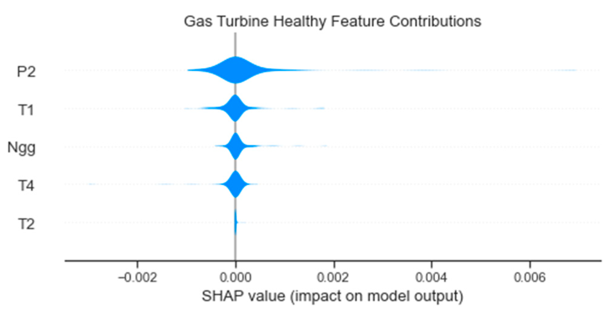
Healthy Data SHAP Global Explanation: The SHAP global explanation for healthy data is presented in Figure 10:
- , , and contribute to prediction according to order of contribution.
- The contributions are almost balanced in both directions, indicating equal total forces that pull the prediction up (healthy side) or pushing it down (failure side).
This explanation is compatible with thermodynamic modelling measures and constitutes the baseline explanation for healthy data prediction.
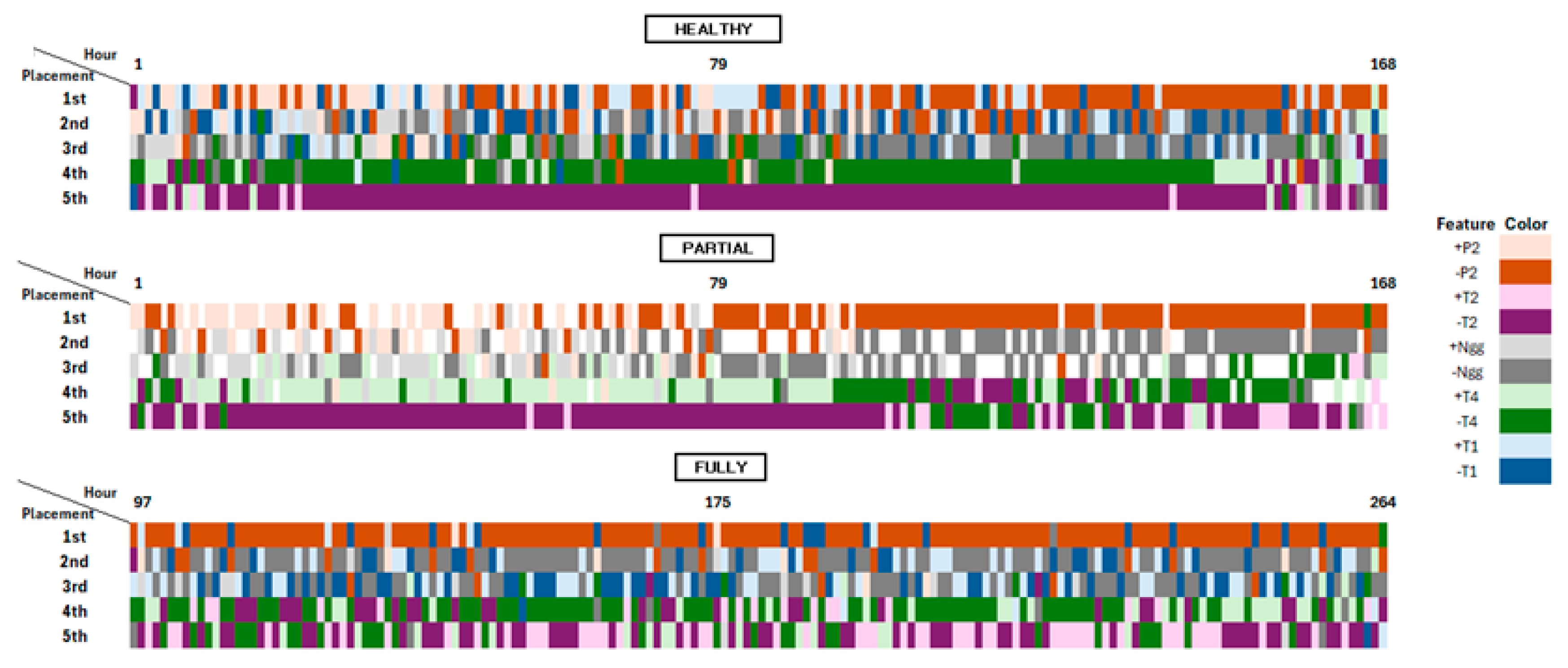
The SHAP local explanation for healthy, partial failure and full failure data are presented in the heatmap Figure 12.
Healthy Data Local Explanation: During this state, features are very volatile, frequently swapping both their ranking and polarity:
- From 1st to 10th hour, and trade the most significant contribution spot. Then trades places with and for second and third contributors.
- From 11th to 166th hour, the system enters a period of high volatility where ,, and frequently swap the top two rankings. Meanwhile, remains the fifth contributor.
- The constant polarity shifts and contribution rank trades suggest a system in operational equilibrium which is typical of a healthy state.
Failure Data Global Explanation: The SHAP global explanation for the partial and full failure data are presented in Figure 11 respectively:
- For both failure modes, contributes the most to prediction followed by , and . This explanation is thus different from the healthy data explanation which points to anomaly.
- For both failure modes the contribution of strongest variables are toward negative directions, which indicates degradation.
- For partial failure, and contributions level increase significantly as data evolves from healthy to failure. and contributions also increase slightly. This is because it takes more contributions to change the state from healthy to failure.
- For full failure, and contributions level decrease significantly as data is completely in failure status. and contributions also decrease slightly. This is because it does not take too much contributions to preserve the failure state.
Figure 11.
Global explanation for failure prediction (a) Partial failure (b) Full failure.
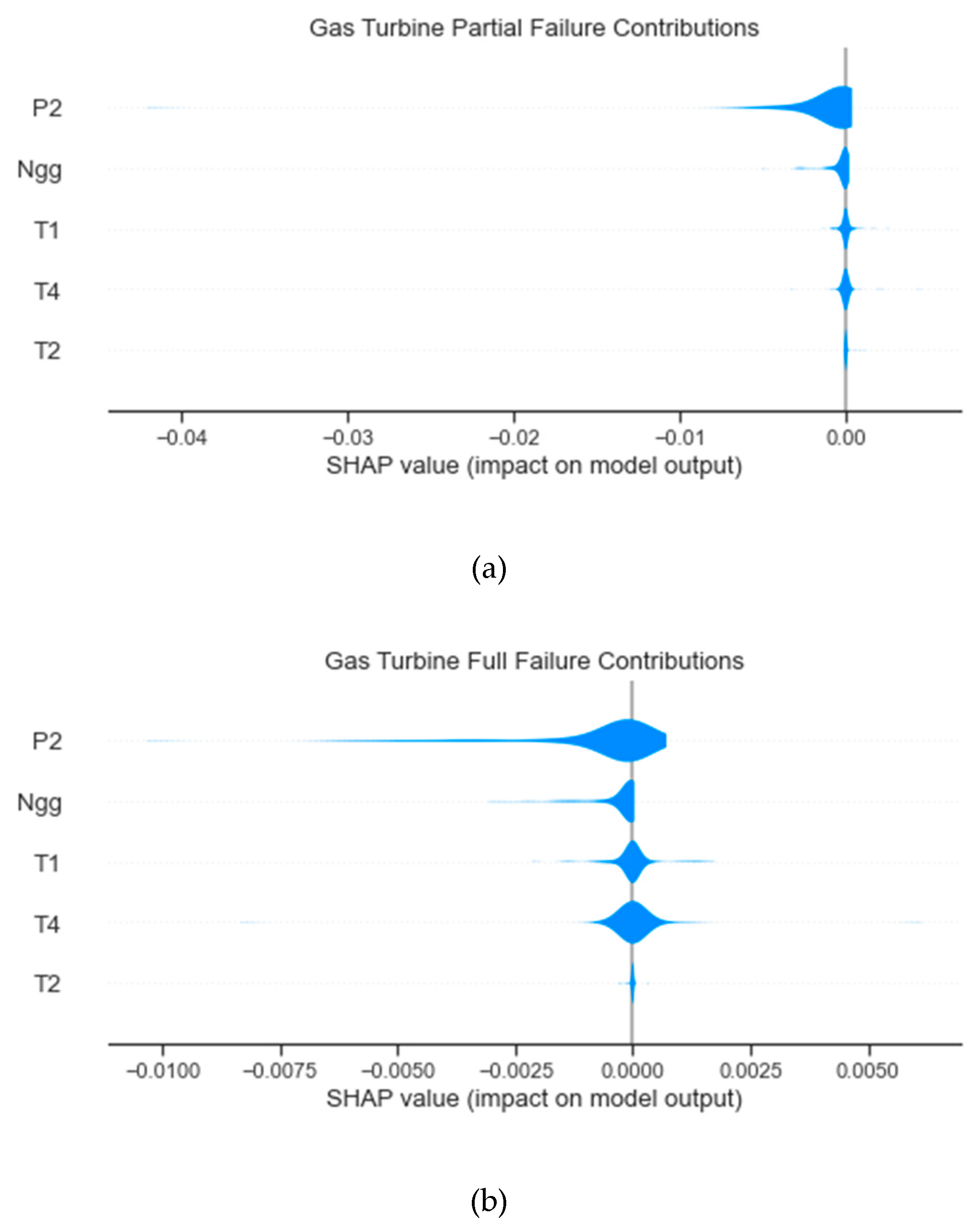
Figure 12.
Local explanation heatmap.
This explanation is compatible with thermodynamic modelling.
Partial Failure Local Explanation: This state shows an initial equilibrium that converges into negative dominance.
- Before 96th hour, the 1st place position is where and +/ frequently trade places.
- and consistently occupy the 2nd and 3rd spots. Their polarities shift often, suggesting the system is attempting to balance fluctuations within the partial failure state.
- Throughout the entire 96-hour sequence, remains almost exclusively in the 5th place ranking.
- After 96th hour, the contribution trend becomes more fixed and is defined by the consistent dominance of negative features.
- The 1st place position settles almost permanently into . Unlike before, there are far fewer instances where and challenge for the top spot.
- transitions from a rotating secondary feature to the nearly permanent 2nd place contributor. This duo of and - defines the late-cycle trend.
- , which was highly influential before 96th hour, begins to drop in the rankings. It moves from the top three to the 4th position and exhibits polarity flips, such as the shift to in the final hours.
- The trend before 96th hour represents a fluctuating partial failure where positive and negative influences from pressure and ambient temperature compete. After 96th hour, the trend transitions into a consistent downward decline led by negative pressure and gas generator speed, with other features losing their relative importance.
Full Failure Local Explanation: This state exhibits the most stable negative contributions in its top ranking until the end sequence:
- From 1st to 167th hour, contributes the most with a dominant negative contribution. Then trades places with and for second and third contributors, though maintains a much more stable presence in the top three.
- Throughout the sequence, and trade third and fourth places with consistent negative contributions.
- The stable negative contributions across pressure, speed, and temperature consistently pull the prediction values lower as the system fails.
G. Explanation Validation with Thermodynamic Equations
In the healthy data modelling, the explanation in Figure 10 shows that:
- , and contribute to prediction according to order of contribution. This explanation is compatible with the thermodynamic modelling. The contributions are almost all balanced in both directions.
- In terms of thermodynamic modelling equation, is proportionate to (7) and values which greatly influenced (8).
- is proportionate to (3) and compressor map) and which influenced .
- , influences and (3) and compressor map) which in turn influence and
- , on the other hand, is inversely proportionate to and (14) which is conditioned by .
- However, influence on is lesser compared to and as there is no direct relationship between and . is just a secondary product of and (7), thus its contribution to is weaker than those features.
In failure prediction, the global explanation in Figure 11 show that:
- and contribute to prediction according to order of contribution. Again, the explanation is compatible with the thermodynamic modelling.
- The global explanation is different from the healthy data explanation, which points to anomaly.
- The contribution of strongest variables are toward negative directions, which also indicates anomaly.
- It also implies that the compressor discharge health parameter, and as the most contributing anomaly features, while and contributions had fallen to 4th and 5th place. This implies an anomaly coming from the compressor.
- Since values decrease over time, the only plausible cause is the decrease of which increases and reduces over time (8).
- reduction, in turn, can only be caused in this case by reduction in compressor pressure ratio, (7), as compressor efficiency is not part of the ML modelling.
- reduction is of course proportionate to and reduction (3) and compressor map).
- Since is conditioned by , will also have to change (14).
- , while having influence on , does not change due to failure injection, thus the weaker contribution compared to and .
The health parameters’ pattern points to compressor failure, where and decrease, which reduces , which in turn lowered value (8) and measures (14). According to local explanations in Figure 12, features contributions are negative, pulling the prediction lower. This indication strengthens the information obtained from the AU level and behavior as well as the predicted HI level.
The transparency of XAI based ML model, which is equivalent to those present in thermodynamic modelling, increases the confidence in ML model utilization. Additionally, by knowing in advance, the components responsible for future failure, maintenance activity and resources can be better organized and optimized. In this case study, it is obvious that the health of the compressor needs to be checked first as the first two most contributing features to failure prediction are and .
V. Conclusion
The goal of this work is to develop an uncertainty aware explainable AI machine learning (ML) model that can predict and confirm the occurrence of gas turbine (GT) failure for preventive maintenance planning. Specifically, Bayesian ML models with (SHAP) explanation capable of life prediction with uncertainty and generating explanation are developed. A 1-year worth of twinspool GT data recording was used for this end. The healthy GT data was estimated using thermodynamic modelling that shows high compatibility with the recorded data. The healthy data was injected with fouling failure and the resultant data was used to train and test the ML model.
A 14-days in advance prediction was executed using healthy and failure testing data. The low uncertainties show that the developed model represents well the data. Consequently, the prediction and explanation of this model can be trusted. The failure life predictions point to anomaly. The uncertainty level shows high possibility of either degraded or failure state, strengthening the life prediction belief.
Consequently, the low and decreasing uncertainty indicator leads to accurate explanations which are compatible with the thermodynamic modelling and point to compressor failure. The explanation points mainly to compressor discharge pressure and gas generator speed reduction which cause decrease in compressor outlet temperature, output power and combustor outlet temperature and all these features contribute negatively to the prediction.
| Nomenclature | ||
| Description | Unit | |
| N | Rotational speed | (RPM) |
| P | Pressure | (kPa) |
| PW | Total power output | (MW) |
| T | Temperature | (°K) |
| Specific heat | (kJ/ kg-K) | |
| Mass flow rate | (kg/hr) | |
| Pressure loss | (kPa) | |
| Air bleed | (kg/h) | |
| Greek Letter | ||
| Efficiency | % | |
| Isentropic index | ||
| Superscript | ||
| Bl | Blowoff | |
| C | Compressor | |
| CC | Combustion chamber | |
| Cor | Corrected | |
| Corc | Corrected using curve | |
| Ed | Exhaust duct | |
| GG | Gas generator | |
| GGT | Gas generator turbine | |
| PT | Power turbine | |
| amb | Ambient condition | |
| 1 | Compressor inlet | |
| 2 | Compressor outlet | |
| 3 | Combustion chamber outlet | |
| 4 | Gas generator outlet | |
| 5 | Power turbine outlet | |
References
- Yu, C. et al., Study on the effects of nanobubble-enhanced diesel spray technology on the performance of heavy-duty gas turbines. Therm. Sci. Eng. Prog. 2026, vol. 73, 104677. [Google Scholar] [CrossRef]
- Hwang, R.; Lee, J.; Kim, J.; Moon, I.; Oh, M. Autonomous Digital Twin Framework for gas turbine combined cycle control loops: Comparative study of proportional-integral control, reinforcement learning, and reinforcement learning with agents. Energy AI 2026, vol. 24, 100727. [Google Scholar] [CrossRef]
- Mohd Irwan Shah, B. S.; Ishak, A. J.; Hassan, M. K.; Norsahperi, N. M. Revolutionizing gas turbine performance analysis with Deep Learning Powered Digital Twin. E-Prime – Nexus Electr. Electron. Intell. Eng. 2026, vol. 17, 201178. [Google Scholar] [CrossRef]
- Zeng, J.; Liang, Z. Predictive group maintenance using probabilistic prognostics and deep reinforcement learning. Comput. Amp Ind. Eng. 2026, vol. 212, 111738. [Google Scholar] [CrossRef]
- Ayman; Onsy, A.; Attallah, O.; Brooks, H.; Morsi, I. Feature learning for bearing prognostics: A comprehensive review of machine/Deep learning methods, challenges, and opportunities. Measurement 2025, vol. 245, 116589. [Google Scholar] [CrossRef]
- Machlev, R. Ev battery fault diagnostics and Prognostics using Deep Learning: Review, Challenges & Opportunities. J. Energy Storage 2024, vol. 83, 110614. [Google Scholar] [CrossRef]
- Cheng, W.; et al. Diagnostics and Prognostics in power plants: A systematic review. Reliab. Eng. Amp Syst. Saf. 2025, vol. 255, 110663. [Google Scholar] [CrossRef]
- Regazzoni, C.; Krayani, A.; Slavic, G.; Marcenaro, L. Probabilistic anomaly detection methods using learned models from time-series data for multimedia self-aware systems. In Advanced Methods and Deep Learning in Computer Vision; 2022; pp. 449–479. [Google Scholar] [CrossRef]
- Schummer, P. et al., Machine learning-based network anomaly detection: Design, implementation, and evaluation. AI 2024, vol. 5(no. 4), 2967–2983. [Google Scholar] [CrossRef]
- Naser, M. Z. Fundamental flaws of physics-informed neural networks and explainability methods in Engineering Systems. Comput. Amp Ind. Eng. 2026, vol. 212, 111704. [Google Scholar] [CrossRef]
- Yuan, X.; Bai, T.; Peng, C. Hybrid modeling method for reactor coolant loop combining data-driven and physics-based constraints. Energy 2026, vol. 345, 140177. [Google Scholar] [CrossRef]
- Ensemble Modeling with a Bayesian Maximal Information Coefficient-Based Model of Bayesian Predictions on Uncertainty Data.
- Explainable AI for industrial fault diagnosis: A systematic review.
- Yang, W. et al., “Survey on Explainable AI: From Approaches, Limitations and Applications Aspects”. Hum.-Cent. Intell. Syst. 2023, vol. 3(no. 3), 161–188. [Google Scholar] [CrossRef]
- S. A. and S. R., “A systematic review of Explainable Artificial Intelligence models and applications: Recent developments and future trends”. Decis. Anal. J. 2023, vol. 7, 100230. [CrossRef]
- Gandhudi, M.; P․J․A․, A.; Srinivas, S.; G․R․, G. Causal inference and explainable artificial intelligence based quantum deep learning for remaining useful lifetime prediction. Knowl.-Based Syst. 2026, vol. 340, 115669. [Google Scholar] [CrossRef]
- Soualhi, M.; Nguyen, K. T. P.; Medjaher, K. Explainable RUL estimation of turbofan engines based on prognostic indicators and heterogeneous ensemble machine learning predictors. Eng. Appl. Artif. Intell. 2024, vol. 133, 108186. [Google Scholar] [CrossRef]
- Qaid, H.; et al. Large language models for explainable fault diagnosis of machines; 2025. [Google Scholar] [CrossRef]
- Forest, F.; Rombach, K.; Fink, O. Interpretable prognostics with concept bottleneck models. Inf. Fusion 2025, vol. 124, 103427. [Google Scholar] [CrossRef]
- Priyadarshini, *!!! REPLACE !!!*. An explainable Autoencoder-based feature extraction combined with CNN-LSTM-PSO model for improved predictive maintenance. Comput. Mater. Amp Contin. vol. 83(no. 1), 635–659, 2025. [CrossRef]
- Razak, M. Y. Industrial Gas Turbines: Performance and Operability; CRC Press: Boca Raton, Cambridge, England; Woodhead Pub, 2008. [Google Scholar]
- Lazzaretto; Toffolo, A. Analytical and Neural Network Models for Gas Turbine Design and Off-Design Simulation. Int. J. Thermodyn. 2001, vol. 4(no. 4), 173–182. [Google Scholar] [CrossRef]
- Razmjooei, M.; Ommi, F.; Saboohi, Z. Experimental Analysis and modeling of gas turbine engine performance: Design Point and off-design insights through system of equations solutions; 2024. [Google Scholar] [CrossRef]
- Zwebek, *!!! REPLACE !!!*; Pilidis, P. “Degradation effects on combined cycle power plant performance: Part 1 — gas turbine cycle component degradation effects,”. In Cycle Innovations; Coal, Biomass and Alternative Fuels, Combustion and Fuels; Oil and Gas Applications, Jun 2001; Volume 2. [Google Scholar] [CrossRef]
- Vivas; Allende-Cid, H.; Salas, R. A systematic review of statistical and Machine Learning Methods for electrical power forecasting with reported MAPE score. Entropy 2020, vol. 22(no. 12), 1412. [Google Scholar] [CrossRef]
- Suradhaniwar, S.; Kar, S.; Durbha, S. S.; Jagarlapudi, A. Time series forecasting of Univariate Agrometeorological Data: A comparative performance evaluation via one-step and multi-step ahead forecasting strategies. Sensors 2021, vol. 21(no. 7), 2430. [Google Scholar] [CrossRef]
- Dash, Ch. S.; Behera, A. K.; Dehuri, S.; Ghosh, A. An outliers detection and elimination framework in classification task of Data Mining. Decis. Anal. J. 2023, vol. 6, 100164. [Google Scholar] [CrossRef]
- Sankar, B.; Shah, B. J.; Jana, S.; Satpathy, R. K.; Gouda, G. Modeling of degradation in gas turbine engine by modified off design simulation. Def. Sci. J. 2022, vol. 72(no. 2), 135–145. [Google Scholar] [CrossRef]
- Hu, M. et al., Digital Twin Model of gas turbine and its application in warning of performance fault. Chin. J. Aeronaut. 2023, vol. 36(no. 3), 449–470. [Google Scholar] [CrossRef]
- Asif, *!!! REPLACE !!!*; et al. A deep learning model for remaining useful life prediction of aircraft turbofan engine on C-MAPSS dataset. IEEE Access 2022, vol. 10, 95425–95440. [Google Scholar] [CrossRef]
- Asif, et al. A deep learning model for remaining useful life prediction of aircraft turbofan engine on C-MAPSS dataset. IEEE Access 2022, vol. 10, 95425–95440. [Google Scholar] [CrossRef]
Figure 1.
Twinspool gas turbine with free power turbine schematic.
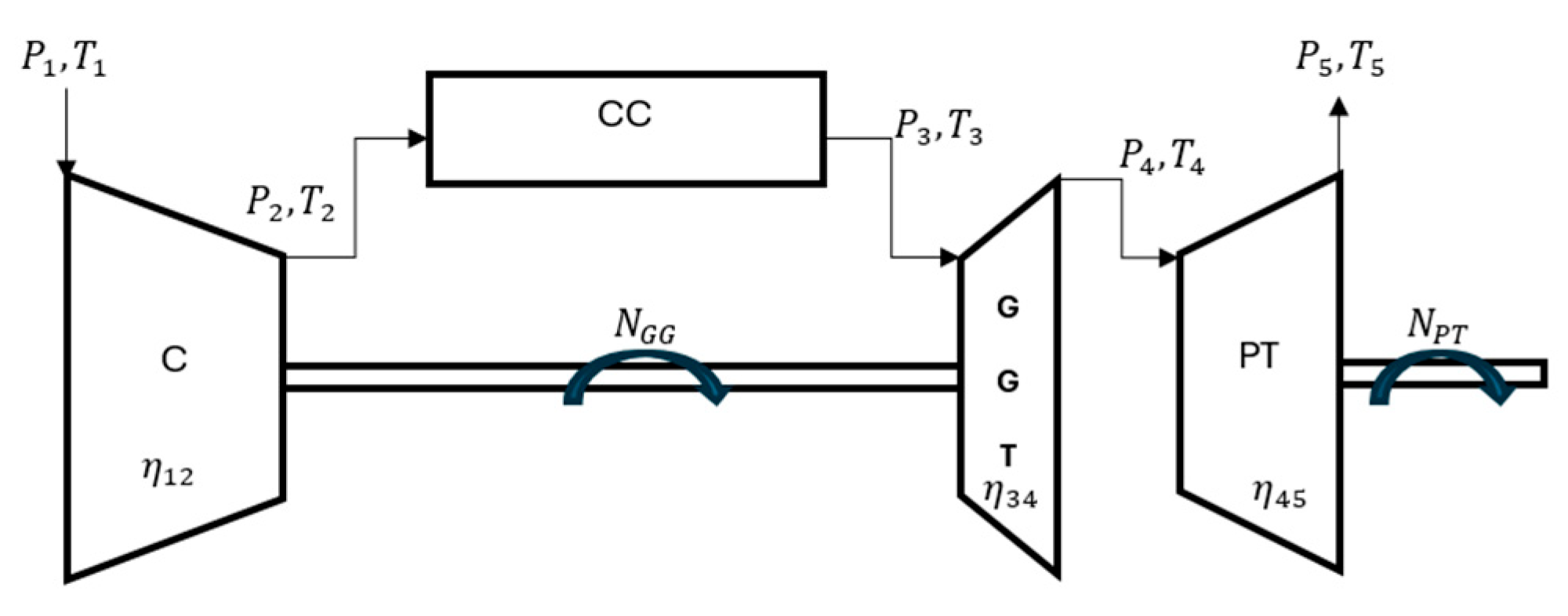
Figure 2.
Compressor component map. (Lazzaretto & Toffolo 2001).
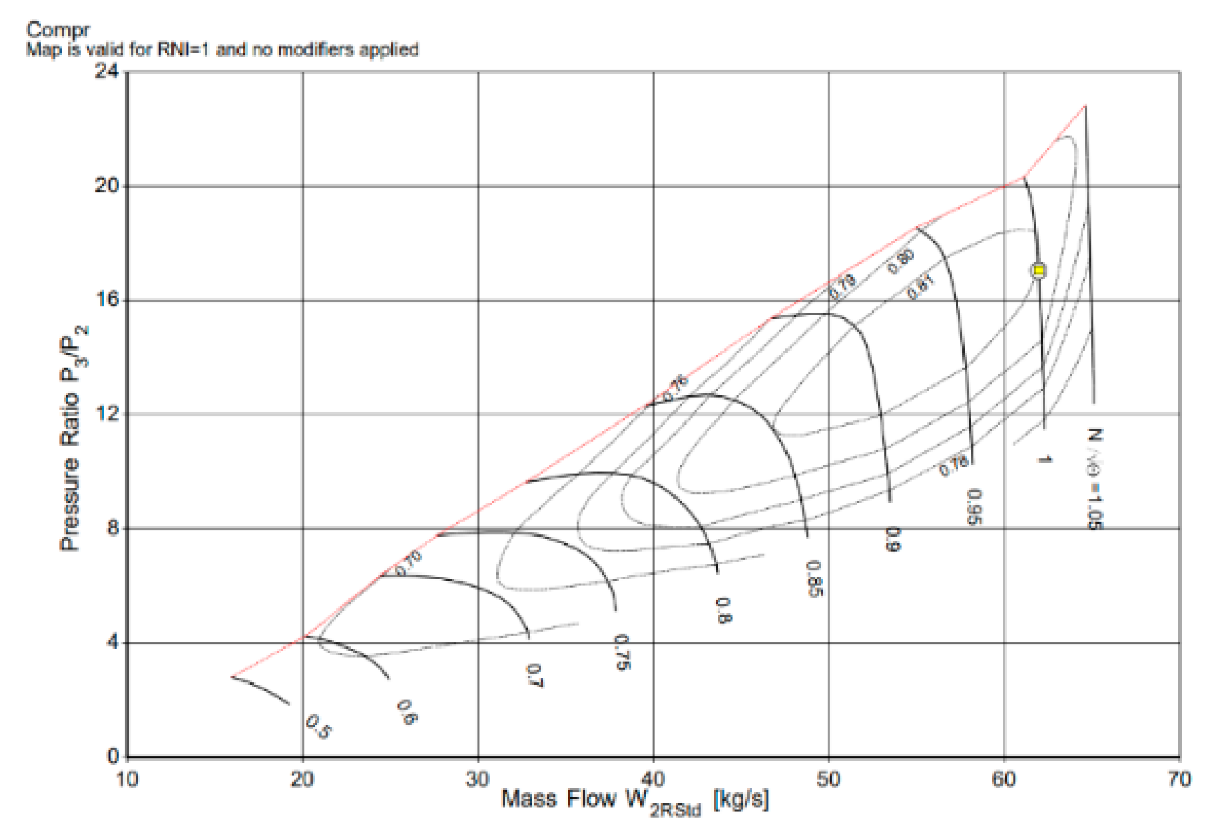
Figure 3.
Bayesian models structures (a)
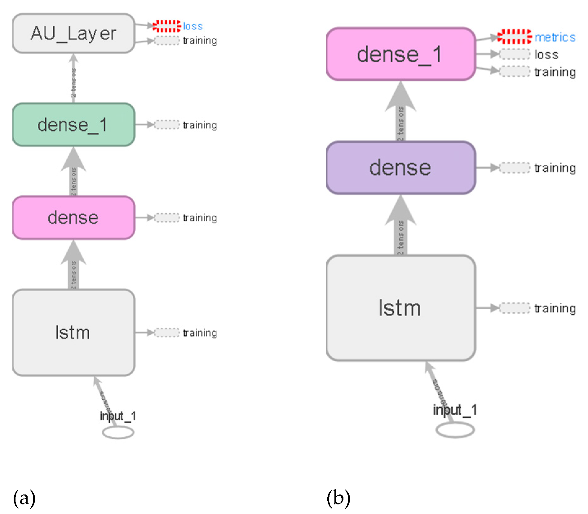
Figure 4.
Explanation models architecture, .
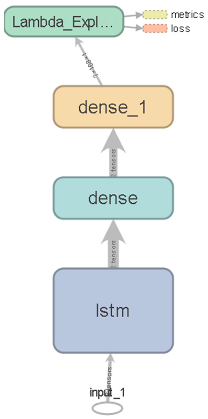
Figure 5.
Predicted vs using thermodynamic modelling.
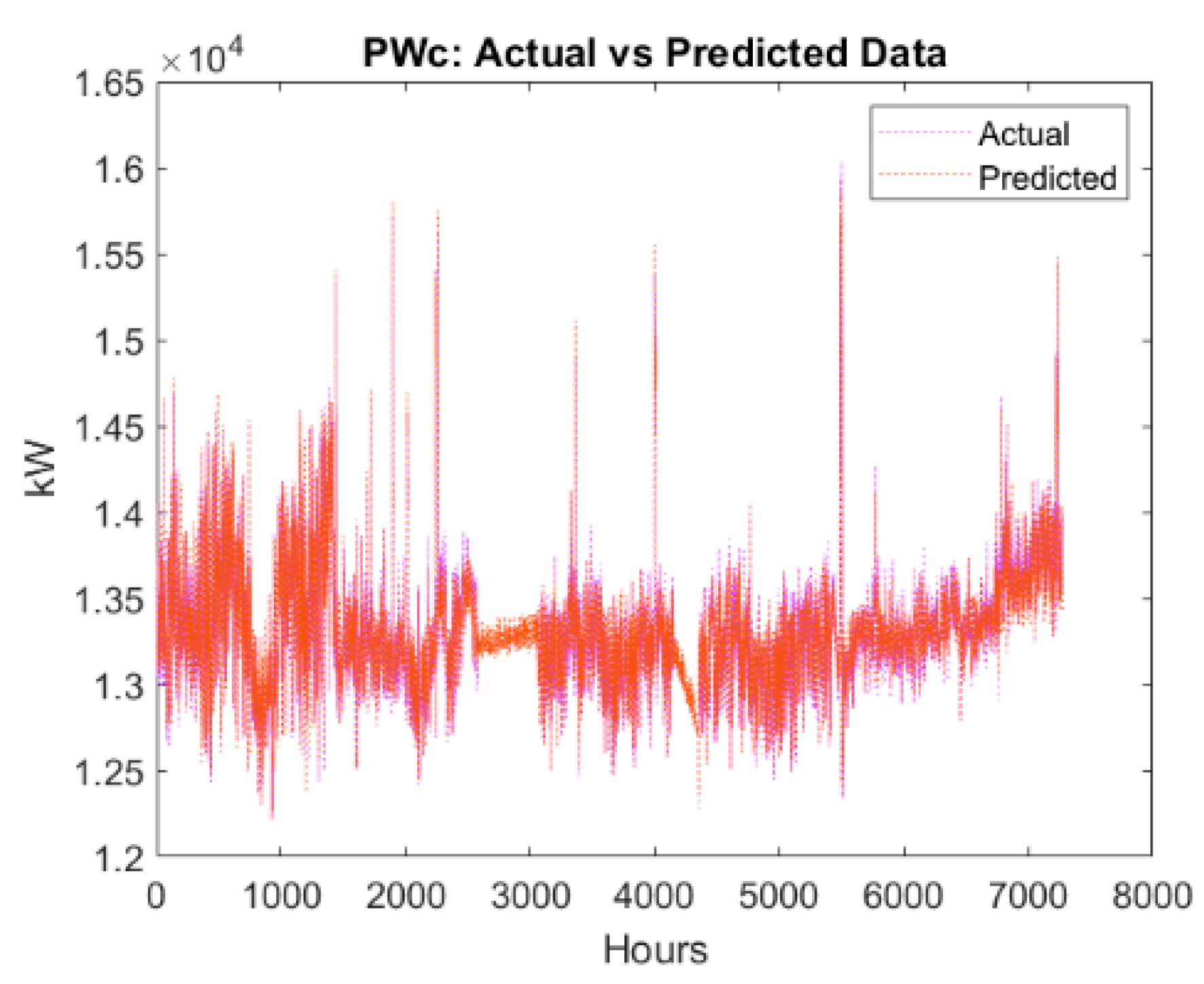
Figure 6.
Piece-wise linear degradation Health Index.
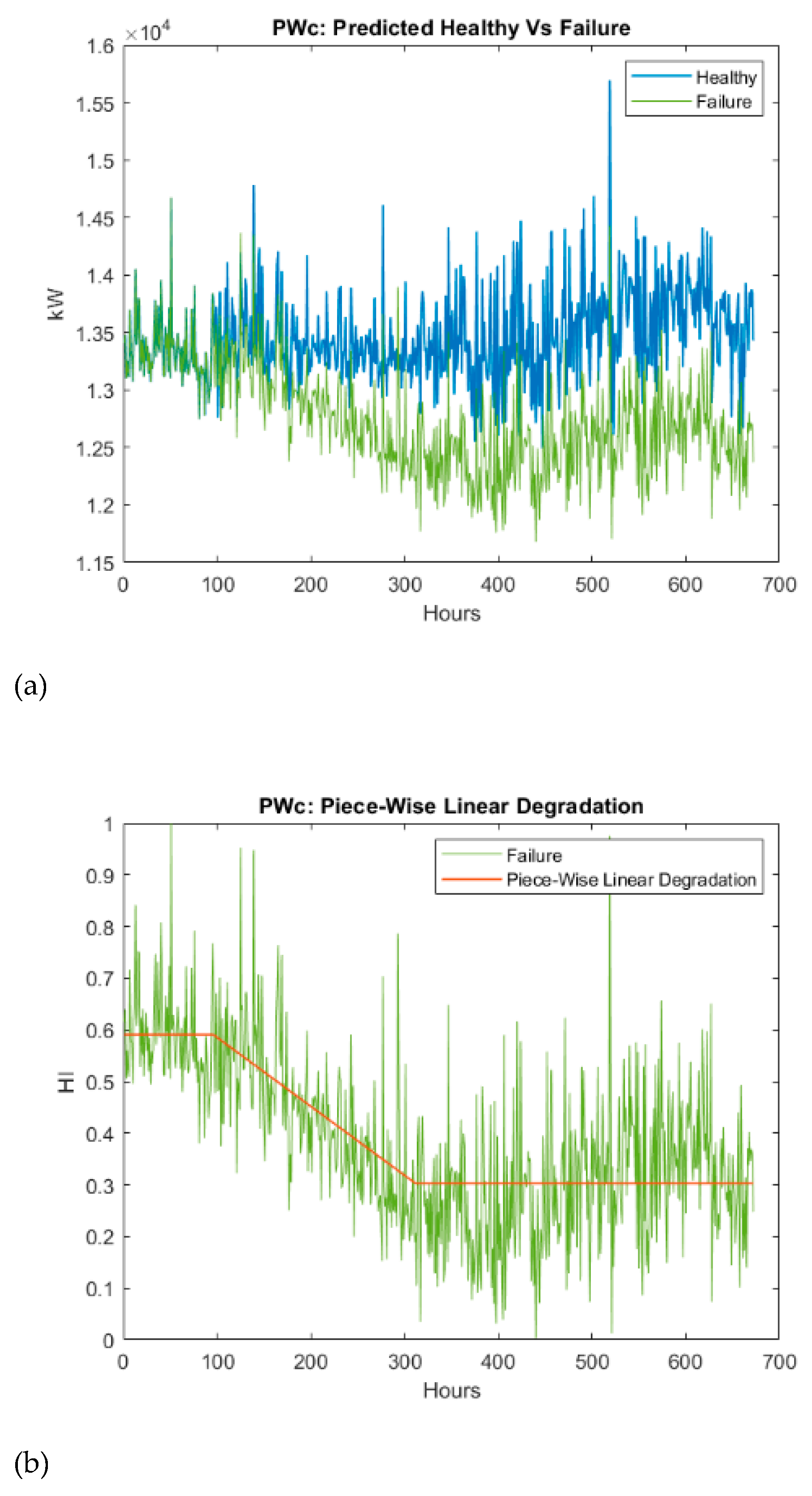
Figure 7.
Healthy data prediction (a) Prediction with aleatoric uncertainty (b) Prediction with epistemic uncertainty.
Figure 7.
Healthy data prediction (a) Prediction with aleatoric uncertainty (b) Prediction with epistemic uncertainty.
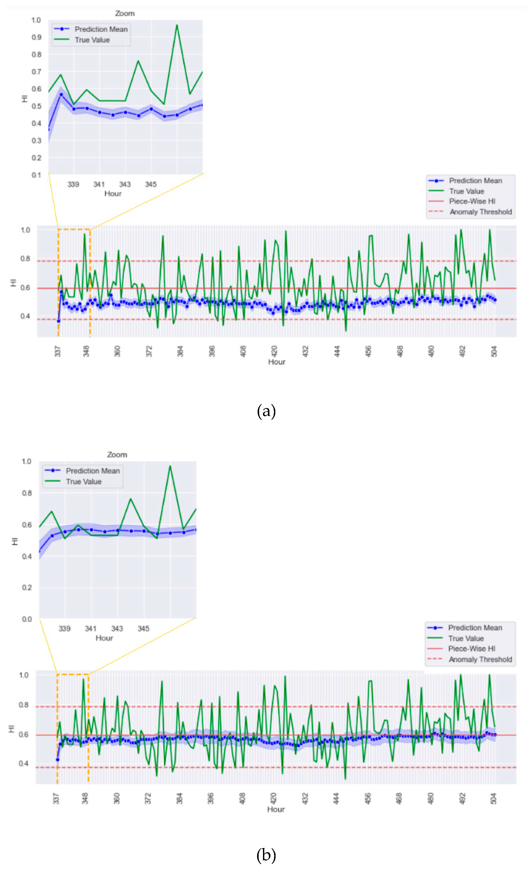
Figure 8.
Partial failure prediction (a) Compared to present data (b) Compared to future data.
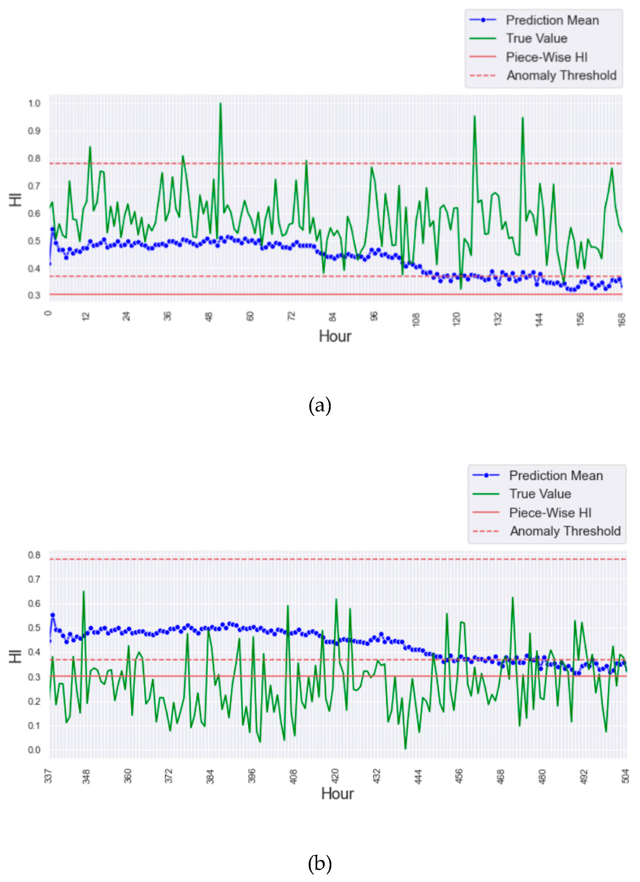
Figure 9.
Full failure prediction (a) Compared to present data (b) Compared to future data.
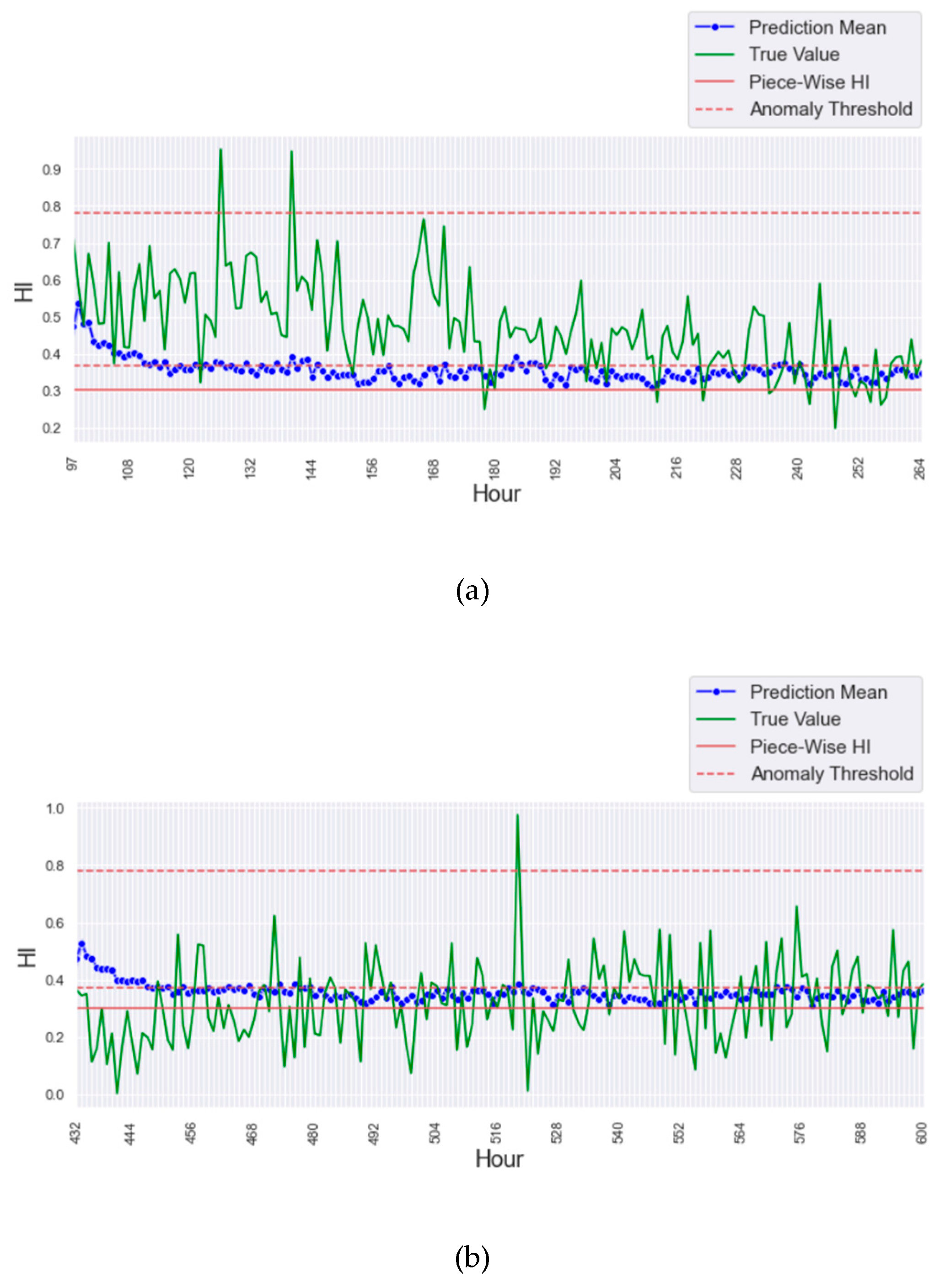
Figure 10.
Global explanation for healthy data modelling.
Disclaimer/Publisher’s Note: The statements, opinions and data contained in all publications are solely those of the individual author(s) and contributor(s) and not of MDPI and/or the editor(s). MDPI and/or the editor(s) disclaim responsibility for any injury to people or property resulting from any ideas, methods, instructions or products referred to in the content. |
© 2026 by the authors. Licensee MDPI, Basel, Switzerland. This article is an open access article distributed under the terms and conditions of the Creative Commons Attribution (CC BY) license (http://creativecommons.org/licenses/by/4.0/).
Copyright: This open access article is published under a Creative Commons CC BY 4.0 license, which permit the free download, distribution, and reuse, provided that the author and preprint are cited in any reuse.


