
Submitted:
27 February 2026
Posted:
03 March 2026
You are already at the latest version
Abstract
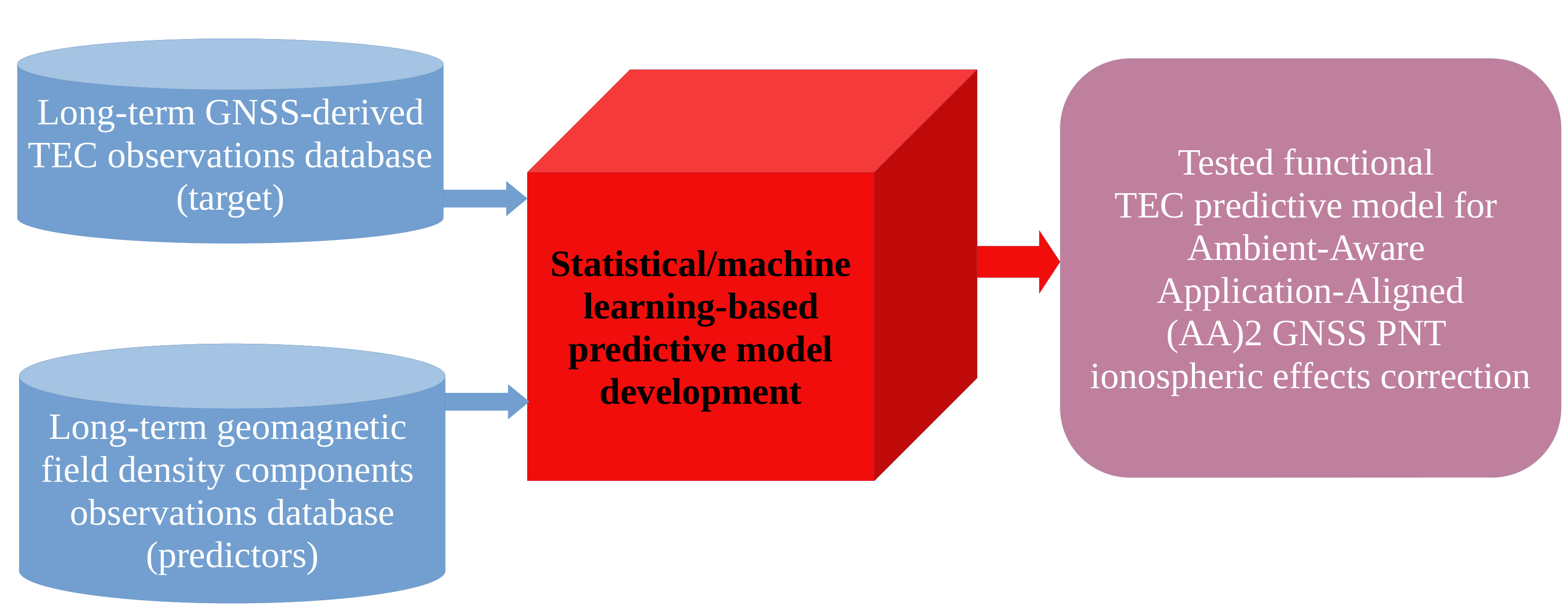
The Global Navigation Satellite System (GNSS) has emerged as a backbone of modern civilisation, industry, and society. Degradations and disruptions of the GNSS Positioning, Navigation, and Timing (PNT) service performance are caused by natural and adversarial sources. The ionospheric effects form the principal single class of the GNSS PNT performance degradation causes. Traditional GNSS ionospheric correction models appear unable to resolve the problem for their global nature, and the intrinsic lack of agility and flexibility. Here we contribute to the case with the proposal of concept and methodology for tailored GNSS ionospheric correction model development in support of GNSS resilience development, based on: (i) a massive dataset of long-term (annual) GNSS-derived total electron content TEC observations, as target variable (ii) a massive dataset of geomagnetic field density components, as predictors, and (iii) utilisation of statistical/machine learning
predictive model development methods. The proposed approach emerges as a component of the previously introduced architecture-agnostic Ambient-Aware Application-Aligned (AA2) GNSS PNT concept, introducing the GNSS positioning environment situation awareness. Proposed concept and methodology is successfully demonstrated in the case of tailored GNSS ionospheric correction model development using the R environment for statistical computing in the case-scenario of mid-latitude single-frequency commercial-grade GNSS rover.
Keywords:
GNSS PNT
; ionospheric effects
; predictive model
; statistical learning
; machine learning
; AmbientAware Application-Aligned (AA2) GNSS PNT
; GNSS observations
; geomagnetic field density
1. Introduction
The Global Navigation Satellite System (GNSS) has become one of the principal cornerstones of modern civilisation, empowering a growing number of technology and socio-economic applications, both systems and services [1,2]. Degradation or disruptions of the GNSS Positioning, Navigation, and Timing (PNT) service result in economic, safety, privacy, and health issues and costs, on levels from the individual to national and international [2]. Maintaining the GNSS PNT performance at levels required by GNSS applications has become the essential task for GNSS operators [1,2], as well as the prime research subject for multidisciplinary teams across the world. Recent developments show the advancement and resilience of the GNSS PNT can be accomplished by utilisation of the Machine Learning (ML)-based models [3] developed on the increasingly available related massive data sets [4,5].
The ionospheric effects, especially the ionospheric delay of a satellite signal as a radio-wave propagation property, have been known as the major natural contributor to the GNSS positioning error, thus degrading its PNT performance [5,6,7,8]. Advanced mitigation of the GNSS PNT ionospheric effects remains the challenge for GNSS researchers, operators, application developers and users, as the standard GNSS ionospheric correction models, such as Klobuchar [8] or NeQuick [9] models, fail to meet demand for robust and resilient GNSS PNT due to their global nature and inability to respond to spatially and temporarily limited ionospheric phenomena affecting the GNSS PNT performance [1,5,7,10,11]. Ionospheric conditions, including radio-wave propagation properties, result from a number of physical and chemical phenomena generated by the space weather effects and others [6,7,8]. The space weather phenomena are of extremely complex nature [6,8,11]. Those have been recently analysed and modelled using ML methods [4,7].
Our group has proposed the Ambient-Aware Application-Aligned GNSS PNT concept [1,12], which exploits the ability of a user mobile GNSS device to collect both the GNSS pseudoranges needed for positioning estimation and the observations of positioning environment, such as observations of geomagnetic field density components, to advance the GNSS PNT resilience against the adversarial natural effects [1,5,12]. Development of a tailored GNSS ionospheric correction model is among the tasks to be completed in the GNSS PNT realisation [1,12]. Here we refer to a proposal for methodology of a bespoke GNSS PNT ionospheric correction model for the GNSS PNT, developed using ML methods applied on experimental geomagnetic indices observations related to GNSS PNT performance, conceived earlier by our group [1]. The proposed methodology has been assessed in this research in the use case of regions in South and Southeast Europe. A number of candidate GNSS PNT ionospheric correction models are developed, their performance assessed, and the optimal model selected and discussed in terms of application in targeted application classes.
The manuscript reads, as follows. This Section introduces the reader to the problem and motivation of the research. Section 2 outlines the research methodology, the ML-based model development methods in particular, and describes the experimental observations taken by the International GNSS Service (IGS) network reference station at Matera, Italy, and the International Real-time Magnetic Observatory Network (INTERMAGNET) reference station at Lonjsko Polje, Croatia, used for development of candidates for the GNSS PNT ionospheric correction model. Section 3 presents results of the model developments and validation, as well as the evidence for selection of the optimal model. Section 4 discusses the research results from the perspectives of the optimal model’s ability to improve the GNSS PNT resilience against the ionospheric effects, and challenges of the model’s deployment, in the GNSS PNT process in particular. This Section provides the concluding remarks, as well as the summarised contributions of the presented research.
2. Materials and Methods
2.1. Dataset Preparation
Data preprocessing, as well as the development and implementation of prognostic models for ionospheric delay, was carried out within the statistical computing environment R [13], supported by specialised packages that facilitate data preparation, machine learning model construction, optimisation, and performance assessment [14,15]. Data necessary for the stated development were obtained from two datasets; one containing estimated values of the total electron content (TEC) and the other containing observations of geomagnetic field density components, both acquired throughout the year 2014.
TEC values are estimated from raw Global Positioning System (GPS) pseudorange observations collected from the International GNSS Data Repository, provided by NASA [16] and further processed using the GPS-TEC program [17]. The data set was obtained from the IGS reference station in Matera (Italy), sampling at 30-second intervals. The components of the geomagnetic field density , , and represent the three orthogonal directions of the geomagnetic field in the Earth’s ionosphere and primarily describe variations in the geomagnetic field. Their values are measured in nanoteslas () and were obtained from the online data repository of the International Real-Time Magnetic Observatory Network (INTERMAGNET) [18]. These components were recorded at the Lonjsko Polje (Croatia) INTERMAGNET reference station with a sampling interval of one minute.
The dataset used in this study was generated by processing raw observation files using an R-based data aggregation and cleaning script. The script iteratively loaded daily records for the year 2014, extracted relevant parameters, and combined them into a unified data structure. For each day, total electron content (TEC) values were read from files in the .Std format, while geomagnetic field density components were already recorded with a one minute sampling interval and did not need additional modifications. Invalid or missing TEC entries, including non-numeric values and measurements less than or equal to zero, were removed to ensure data integrity. Additionally, records containing placeholder values (99,999) in any geomagnetic field component were excluded. The resulting merged dataset contains 523,700 individual observations and includes the parameters DATE, TIME, Bx, By, Bz, and TEC. Statistical analysis of the refined dataset yielded a mean TEC value of 13.37, a standard deviation of 10.00, and a variance of 100.05, indicating a consistent and physically plausible distribution of measurements suitable for subsequent model development and validation.
Figure 1 displays the density plot and the normal distribution of the TEC values from the refined data set. The observed distribution is asymmetrical, with lower values being prevalent, and deviates from a normal distribution, which highlights the need for a model capable of capturing the non-linear relationships and heterogeneity within the data.
Figure 2 presents the median, interquartile range, and outliers for both predictors , & and the target value TEC where it is evident that most of the data are concentrated within the lower range (0 to 20 TECU), indicating that most of the measurements occurred under stable ionospheric and geomagnetic conditions. The intercorrelations between the variables were analysed, with the result shown in Figure 3, where a notable correlation was observed; 0.73 between and . This value suggests a moderate to strong correlation, which is generally sufficient to have a visible impact on the development and performance of the prognostic model, so it was taken into account when developing the models.
2.2. Models
The previously described dataset was randomly divided into two subsets, a training set and a testing set, in a ratio of 80% to 20%, respectively. Such a division is necessary to mitigate the issue of overfitting, which would hinder models’ effective generalisation to new, unseen data. This partitioning ensures that each developed model is trained and evaluated on identical datasets, facilitating fair and consistent model evaluation while eliminating potential biases stemming from differing input data.
The development of a prognostic model m for TEC ionospheric delay using magnetic field components , , and as predictors can be generalised, as shown in Equation (1).
2.2.1. Linear Regression
Linear regression represents a fundamental statistical machine learning model used for predicting continuous values, operating by modelling the linear relationship between one or more independent variables and a dependent variable, which represents the target value of interest. The linear regression model seeks to determine the coefficients , , , and for the predictor variables , , and the mutual interaction effect (motivated by the results of the prior correlation analysis) while minimising the discrepancy between observed and predicted values. The function implemented in the model is shown in 2, where denotes the intercept constant and denotes the random error (residual) and is based on the principles of linear statistical models outlined in [19].
2.2.2. Decision Tree
The decision tree model is based on a hierarchical structure that represents a series of binary decisions, with each decision directing the data toward one of the two subtrees. The algorithm in this approach involves recursively partitioning the data into progressively smaller subsets through a sequence of simple decision rules, represented as tree nodes, until a final prediction, represented as tree’s leaf nodes, is reached [20].
2.2.3. Gradient Boosting
The gradient boosting model represents an ensemble learning approach that sequentially combines multiple weak learners, typically decision trees, to form a strong predictive model. Each new tree is trained to minimise the residual errors of the previous ensemble, thereby progressively improving prediction accuracy through an additive optimisation process [21]. This method is particularly effective for capturing complex nonlinear dependencies between input variables and the target output, while maintaining high flexibility in model fitting.
The training process involved 2000 sequential trees (n.trees = 2000) with a maximum interaction depth of 16 (interaction.depth = 16), allowing the model to learn high-order feature interactions. A shrinkage factor of 0.4 (shrinkage = 0.4) was applied to control the learning rate and reduce overfitting, while 12-fold cross-validation (cv.folds = 12) was used to ensure model robustness and generalisation. By iteratively refining predictions through gradient-based optimisation, the gradient boosting model achieves a balanced trade-off between accuracy and computational complexity.
2.2.4. Random Forest
The random forest model is an ensemble learning technique that constructs a large number of decision trees during training and outputs the average prediction of all individual trees for regression tasks. By introducing randomness both in the selection of data subsets and feature subsets used for node splitting, the random forest effectively reduces overfitting and variance compared to a single decision tree, resulting in improved model stability and generalisation [22].
The forest consisted of 100 decision trees (ntree = 100), each trained on randomly sampled subsets of the training data. This configuration allowed the model to balance predictive accuracy with computational efficiency while ensuring adequate representation of underlying data variability.
2.2.5. K Nearest Neighbors
The K-nearest neighbors (KNN) model is a non-parametric, instance-based learning algorithm that performs predictions by analyzing the proximity of data points within the feature space. Unlike parametric models, KNN does not rely on an explicit functional form; instead, it infers the target value of a new observation based on the average of the target values of its K nearest neighbors in the training dataset. This property allows KNN to effectively model nonlinear relationships between predictors and the response variable but at the cost of higher computational demands, especially for large datasets [23].
Model training was performed using a repeated 10-fold cross-validation scheme (method = "repeatedcv", number = 10, repeats = 5), ensuring robustness and reducing the risk of overfitting. The optimal number of neighbors (K) was determined automatically by testing 10 candidate configurations (tuneLength = 10) and selecting the one yielding the best validation performance. Due to its instance-based nature, the KNN model requires substantially more computational time compared to tree-based and linear models.
2.2.6. Neural Network
The neural network model is a data-driven machine learning approach capable of capturing highly complex and nonlinear relationships between input and output variables through interconnected layers of artificial neurons. Each neuron performs a weighted summation of its inputs followed by the application of an activation function, allowing the model to learn intricate mappings between predictor variables and target response [24].
The feedforward neural network architecture consisted of two hidden layers, each containing 64 neurons with rectified linear unit (ReLU) activation functions (activation = ’relu’), and a single output neuron for predicting the TEC. The model was compiled using the root mean square propagation optimizer (optimizer_rmsprop) and the mean squared error loss function (loss = ’mse’), with mean absolute error (mae) tracked as an additional performance metric.
2.3. Model Evaluation
The developed TEC prediction models are evaluated based on three key criteria:
- 1.
- Predicted vs. Observed (P-O) diagram alongside with the Probability-Probability diagram (P-P),
- 2.
- Root mean square error (RMSE),
- 3.
- Adjusted .
The P-O diagram offers a visual comparison of predicted and observed outcomes, where the ideal line is an indicator of perfect prediction, while the P-P diagram graphically represents the comparison between the cumulative distribution of predicted values and the cumulative distribution of observed values. The P-O diagram provides insight into the accuracy of individual predictions compared to observed values of TEC, commonly known as goodness-of-fit, whereas the P-P diagram illustrates whether the model’s predicted TEC values follow the same distribution as the observed values. The root mean square error (RMSE) is used to measure the average magnitude of the error between predicted and observed values, highlighting the model’s overall predictive accuracy along with systematic biases inherent to the considered phenomenon. RMSE is calculated according to 3, where are the observed values, are the predicted values, and n is the number of observations.
The adjusted coefficient of determination () is derived from the standard coefficient of determination (determined using (4), with being the mean of the observed values), which indicates how well the model can describe the original variance contained within the data set.
The improves on the standard coefficient of determination by incorporating penalties for the inclusion of excessive predictors p, thus reducing the likelihood of model overfitting. The calculation of the is shown in (5).
In addition to the aforementioned three key criteria, to gain a comprehensive understanding of each model’s qualities from different perspectives [25], two more metrics were recorded for each model: (i) maximum residual value, which represents the largest single error among all predicted values and (ii) model development time expressed in seconds.
3. Results
The model performance assessment described in Section 2.3 was applied to six TEC prediction models developed to allow a thorough comparative analysis. The evaluation results for each model are summarized in Table 1.
The linear regression model expectedly demonstrated the shortest development time, a result of the nature of the algorithm’s operation. This highly efficient computability comes at the cost of poor prediction accuracy, with its RMSE, , and maximal residual values being the lowest performing among the developed models.
In contrast, the random forest and gradient boosting models provided substantially better fit to the data, with RMSE values of 4.91 TECU and 5.73 TECU, respectively, and values exceeding 0.72. While the random forest achieved slightly lower average prediction errors, the gradient boosting model demonstrated improved ability to limit large individual residuals, achieving the lowest maximal residual value among the ensemble methods (36.85 TECU).
The KNN model exhibited the highest overall predictive performance, attaining an RMSE of 4.64 TECU and an of 0.865, albeit at the cost of considerably longer development time (18 274.81 s). The precision of this model highlights the effectiveness of instance-based learning in capturing complex nonlinear relationships between geomagnetic field components and TEC variations.
According to the model evaluation criteria defined in Section 2.3, the KNN model achieved the best overall balance between predictive precision and variance explanation, while the gradient boosting model remained the most effective among the ensemble-based approaches. Given its highest and lowest RMSE, the KNN model was therefore selected as the most accurate and reliable predictor of TEC values within the analysed dataset.
Figure 4 depicts each model’s P-O diagram, revealing a relatively large dispersion of prediction points in each diagram, with some predictions, like those of gradient boosting and neural network models, extending into negative TEC values; an occurrence that is inherently impossible.
The systematic underprediction at lower values, as displayed by each model’s P-P diagram in Figure 5, suggests that the models may struggle with extreme values of the distribution, reducing their reliability in such instances. The behaviours observed in the graphical analysis of the above-mentioned figures suggest that systematic deviations may arise from the inherent data distribution, indicating that the issue could be related to shared underlying assumptions or data preprocessing steps rather than being specific to the architecture of any individual model.
4. Discussion
Presented research aimed at development of a single all-purpose statistical learning-based GNSS ionospheric correction model. The model is anticipated to predict the TEC, a GNSS environmental variable that determines the GNSS ionospheric delay, based on the yearlong set of experimental observations. The rationale behind utilisation of the annual data set lies in presumption that during that time-span observations are available for all kinds of space weather events affecting the GNSS PNT performance, with proportional frequency of occurrence. Additionally, the experimental GNSS observations used for model development were collected in the mid-latitude region with numerous GNSS-related applications users, thus establishing a valuable case for the GNSS ionospheric error/delay correction model development.
The original data set is split into training and testing sub-sets without further classification based on the intensity levels of the space weather events affecting the GNSS PNT performance. The presented approach is embraced to yield a single all-purpose climatological model of the TEC, given the assumed real cases of space weather events, with the proportional rates of occurrence.
Methods for learning-based model development were selected in consideration of statistical properties of both the target (TEC value) and predictors (Bx, By, Bz). Several candidate models are developed, and assessed for their performance in terms of: (i) ability to describe the bias in TEC values, assessed through analysis of RMSE, and Maximum of residuals ( - ) (ii) ability to describe variance in TEC values, assessed through the analysis of and (iii) ability to offer linear P-O diagram, thus allowing for sustained errors across the range of target variable values (TEC). Additionally, model development time is assessed to infer suitability to be deployed on a small GNSS devices/processes with limited power and computational resources.
The Linear Regression Model emerges as the worst performer out of six candidates. Although it extends the smallest Maximum of residuals, other performance indicators are well beyond the competitors. More advanced Decision Tree and Neural Network Models, respectively, develop in a reasonably fast manner but extend far insufficient performance indicators. More computationally extensive and, the structurally complex Gradient Boosting, and Random Forest, in particular, provide a reasonable performance with the proportionally extended development time.
The KNN Model emerges as the unquestionable winner. It extends the second lowest Maximum of residuals, after the Linear Regression Model, the lowest RMSE, and an impressive , confirming the ability to describe more than 86% of the variance contained in the original dataset.
The approach of developing a single all-purpose model takes its toll in the general lack of linearity in P-O diagrams of all contenders. The KNN Model and Neural Network Models appear as winners, considering the P-O diagram criterion.
This manuscript introduces and demonstrates a new methodology for customised/tailored GNSS ionospheric correction model development based on the experimental observations of the GNSS environmental (geomagnetic field density) conditions. In such terms, the GNSS ionospheric correction model based on statistical learning and situation awareness renders suitable for implementation in the GNSS PNT.
Consideration of a single annual data set taken at the single reference point asks for continuation of the research in which the will be assessed for their spatio-temporal (geographic, seasonal, Solar Maxima etc.) performance. Additionally, the methodology for geomagnetic data quality and integrity assurance is to be developed, thus preventing and mitigating potential adversarial spoofing attacks on GNSS ionospheric model development and, consequently, on GNSS PNT performance.
5. Conclusions
Ionospheric effects remain the major source of GNSS PNT performance degradation, affecting the dominant class of single-frequency GNSS PNT users across disciplines and domains of applications. Here, a new approach in the GNSS ionospheric correction model development and deployment is introduced, based on long-term GNSS and geomagnetic field density observations and utilisation of the statistical learning-based model development approach. Proposed methodology is demonstrated in the case scenario of the GNSS ionospheric correction model development based on a single location annual set of observations. The KNN model emerges as the optimal statistical learning-based TEC prediction model. It features a consistent and advanced correction ability, with the lowest RMSE, the lowest RMSE/Maximum of residuals ratio, and the respectable ability to describe more than 86% of the variance in the original data.
The new approach proposed in the GNSS ionospheric correction modelling has significant prospects for utilisation in a wide range of GNSS PNT services, including distributed Positioning-as-a-Service and GNSS PNT.
The research will continue with addressing the spatio-temporal performance and sustainability of the novel statistical learning-based GNSS ionospheric correction model, as well as with the resilience development against the adversarial geomagnetic spoofing attacks on both the models and the resulting GNSS PNT performance.
Author Contributions
R.F. conceived the study; M.P. and S.D. prepared the problem statement and assessed the state-of-the-art research; R.F., M.P. and L.M. developed the methodology and the tailored software in the R environment for statistical computing; M.P. and S.D. aggregated and pre-processed sets of observations using performed exploratory statistical analysis, analysed statistical learning-based model development methods and performed research in accordance with the methodology set and utilising the R-based tailored software. All authors contributed to the discussion of the results and the formulation of the conclusion. R.F. and M.P. contributed equally to the presented work. All authors have read and agreed to the published version of the manuscript.
Funding
This research received no external funding.
Data Availability Statement
The processed data used in this study are available at https://github.com/MPetranovic/gnss-ionospheric-correction-models-article-data. Raw data were obtained from [16,18].
Conflicts of Interest
The authors declare no conflicts of interest.
Abbreviations
The following abbreviations are used in this manuscript:
| GNSS | Global Navigation Satellite System |
| PNT | Positioning, Navigation, and Timing |
| TEC | Total Electron Content |
| Ambient-Aware Application-Aligned | |
| ML | Machine Learning |
| IGS | International GNSS Service |
| INTERMAGNET | International Real-time Magnetic Observatory Network |
| GPS | Global Positioning System |
| KNN | K-Nearest Neighbors |
| ReLU | Rectified Linear Unit |
| P-O | Predicted vs. Observed |
| P-P | Probability-Probability |
| RMSE | Root Mean Square Error |
| Adjusted Coefficient of Determination |
References
- Filjar, R. An application-centred resilient GNSS position estimation algorithm based on positioning environment conditions awareness. Proc. ION ITM 2022, Long Beach, CA, USA, 2022; pp. 1123–1136. [Google Scholar] [CrossRef]
- Flytkjær, R.; et al. The economic impact on the UK of a disruption to GNSS; London Economics: London, UK, 2023; Available online: https://londoneconomics.co.uk/blog/publication/the-economic-impact-on-the-uk-of-a-disruption-to-gnss-2021/ (accessed on 21 August 2025).
- Efron, B.; Hastie, T. Computer Age Statistical Inference: Algorithms, Evidence, and Data Science; Cambridge University Press: Cambridge, UK, 2021; ISBN 978-1108823418. [Google Scholar]
- Mohanty, A.; Gao, G. A Survey of Machine Learning Techniques for Improving Global Navigation Satellite Systems. EURASIP Journal on Advances in Signal Processing 2024, 73. [Google Scholar] [CrossRef]
- Oxley, A. Uncertainties in GPS Positioning: A Mathematical Discourse; Academic Press: London, UK, 2017; ISBN 978-0-12-809594-2. [Google Scholar]
- Davies, K. Ionospheric Radio; Peter Peregrinus Ltd.: London, UK, 1990; ISBN 978-0863411861. [Google Scholar]
- Filić, M.; Filjar, R. Modelling the Relation between GNSS Positioning Performance Degradation, and Space Weather and Ionospheric Conditions using RReliefF Features Selection. Proc. 31st Int. Tech. Meeting ION GNSS+ 2018, Miami, FL, USA, 2018; pp. 1999–2006. [Google Scholar] [CrossRef]
- Klobuchar, J.A. Ionospheric Time-Delay Algorithm for Single-Frequency GPS Users. IEEE Trans. Aerospace and Electronic Systems 1987, AES-23(3), 325–331. [Google Scholar] [CrossRef]
- European Commission. Ionospheric Correction Algorithm for Galileo Single Frequency Users, version 2; European Commission: Bruxelles, Belgium, 2016; Available online: https://www.gsc-europa.eu/sites/default/files/sites/all/files/Galileo_Ionospheric_Model.pdf (accessed on 21 August 2025).
- Camporeale, E. The Challenge of Machine Learning in Space Weather: Nowcasting and Forecasting. Space Weather 2019, 17(8), 1166–1207. [Google Scholar] [CrossRef]
- Chandrokar, H.M. Machine Learning in Space Weather: Forecasting, Identification & Uncertainty Quantification. Ph.D. Thesis, Eindhoven University of Technology, Eindhoven, The Netherlands, 2019. [Google Scholar]
- Filjar, R.; Hedji, I.; Prpić-Oršić, J.; Iliev, T.B. An ambient-adaptive GNSS TEC predictive model for short-term rapid geomagnetic storm events. Remote Sens. 2024, 16(16), 3051. [Google Scholar] [CrossRef]
- R Core Team. R: A Language and Environment for Statistical Computing. R Foundation for Statistical Computing, Vienna, Austria, 2024; Available online: https://www.r-project.org/ (accessed on 8 August 2025).
- Kuhn, M. The caret package. Available online: https://topepo.github.io/caret/ (accessed on 8 August 2025).
- Kuhn, M. Building predictive models in R using the caret package. Journal of Statistical Software 2008, 28(5), 1–26. [Google Scholar] [CrossRef]
- NASA Earthdata portal. Available online: https://www.earthdata.nasa.gov/ (accessed on 8 August 2025).
- Seemala, G.K. Estimation of ionospheric total electron content (TEC) from GNSS observations. In Atmospheric Remote Sensing; Elsevier: Amsterdam, The Netherlands, 2023; pp. 63–84. [Google Scholar] [CrossRef]
- INTERMAGNET. Data repositories. Available online: https://github.com/orgs/INTERMAGNET/repositories (accessed on 8 August 2025).
- Chambers, J.M.; Hastie, T. Statistical models in S; Wadsworth & Brooks/Cole: Pacific Grove, CA, USA, 1992. [Google Scholar]
- Breiman, L.; Friedman, J.H.; Olshen, R.A.; Stone, C.J. Classification and Regression Trees; Chapman & Hall/CRC: Boca Raton, FL, USA, 1998. [Google Scholar]
- Hastie, T.; Tibshirani, R.; Friedman, J. The Elements of Statistical Learning: Data Mining, Inference, and Prediction, 2nd ed.; Springer Nature: Cham, Switzerland, 2017; pp. 358–361. ISBN 978-0387848570. [Google Scholar]
- Louppe, G. Understanding random forests: from theory to practice. Ph.D. Thesis, University of Liège, Liège, Belgium, 2014. [Google Scholar] [CrossRef]
- James, G.; Witten, D.; Hastie, T.; Tibshirani, R. An Introduction to Statistical Learning: With Applications in R, 2nd ed.; Springer Nature: Cham, Switzerland, 2021; pp. 39–42. ISBN 978-1461471370. [Google Scholar]
- Boehmke, B.; Greenwell, B. Hands-On Machine Learning with R; CRC Press: Boca Raton, FL, USA, 2020; pp. 247–270. ISBN 978-1138495685. [Google Scholar]
- Biecek, P.; Burzykowski, T. Explanatory Model Analysis: Explore, Explain, and Examine Predictive Models; CRC Press: Boca Raton, FL, USA, 2021; ISBN 9780367135591. [Google Scholar]
Figure 1.
Data density (blue bars and line) and normal distribution (pink dashed line) of the refined data.
Figure 1.
Data density (blue bars and line) and normal distribution (pink dashed line) of the refined data.

Figure 2.
Box plots of the analysed variables: (a) total electron content (TEC); (b) geomagnetic field component ; (c) geomagnetic field component ; and (d) geomagnetic field component .
Figure 2.
Box plots of the analysed variables: (a) total electron content (TEC); (b) geomagnetic field component ; (c) geomagnetic field component ; and (d) geomagnetic field component .

Figure 3.
Correlogram of the used dataset.

Figure 4.
P-O diagrams of the evaluated TEC prediction models: (a) linear regression; (b) decision tree; (c) gradient boosting; (d) random forest; (e) KNN; and (f) neural network. The reference line, indicating perfect prediction, is shown in pink.
Figure 4.
P-O diagrams of the evaluated TEC prediction models: (a) linear regression; (b) decision tree; (c) gradient boosting; (d) random forest; (e) KNN; and (f) neural network. The reference line, indicating perfect prediction, is shown in pink.

Figure 5.
P-P diagrams of the evaluated TEC prediction models: (a) linear regression; (b) decision tree; (c) gradient boosting; (d) random forest; (e) KNN; and (f) neural network. The reference line, indicating perfect prediction, is shown in pink.
Figure 5.
P-P diagrams of the evaluated TEC prediction models: (a) linear regression; (b) decision tree; (c) gradient boosting; (d) random forest; (e) KNN; and (f) neural network. The reference line, indicating perfect prediction, is shown in pink.


Table 1.
Performance assessment results of models.
| Model | RMSE [TECU] | Max. Residual [TECU] | Adj. [%] | Development Time [s] |
|---|---|---|---|---|
| Linear regression | 9.001426 | 30.763 | 0.1884 | 0.04 |
| Decision tree | 8.273675 | 36.408 | 0.3157607 | 0.07 |
| Gradient boosting | 5.730889 | 36.85178 | 0.7445679 | 3663.85 |
| Random forest | 4.911834 | 40.83849 | 0.7293617 | 4414.39 |
| K-nearest neighbors | 4.638222 | 35.14286 | 0.8646796 | 18274.81 |
| Neural network | 7.125561 | 37.7001 | 0.4954369 | 703.42 |
Disclaimer/Publisher’s Note: The statements, opinions and data contained in all publications are solely those of the individual author(s) and contributor(s) and not of MDPI and/or the editor(s). MDPI and/or the editor(s) disclaim responsibility for any injury to people or property resulting from any ideas, methods, instructions or products referred to in the content. |
© 2026 by the authors. Licensee MDPI, Basel, Switzerland. This article is an open access article distributed under the terms and conditions of the Creative Commons Attribution (CC BY) license (http://creativecommons.org/licenses/by/4.0/).
Copyright: This open access article is published under a Creative Commons CC BY 4.0 license, which permit the free download, distribution, and reuse, provided that the author and preprint are cited in any reuse.


