
Submitted:
26 February 2026
Posted:
28 February 2026
You are already at the latest version
Abstract
The Standard Model is a renormalizable chiral Yang–Mills–Higgs quantum field theory defined on a principal fiber bundle over four-dimensional Minkowski spacetime with structure group GSM = SU(3)C × SU(2)L × U(1)Y. Its Lagrangian is uniquely constrained by local gauge invari-ance, Lorentz symmetry, perturbative renormalizability, and the requirement of gauge and mixed anomaly cancellation. The resulting theory couples non-Abelian gauge connections to chiral fermions transforming in complex representations of su(3) ⊕ su(2) ⊕ u(1), together with a scalar Higgs doublet whose vacuum expectation value induces spontaneous symmetry breaking and mass generation through the Higgs mechanism. In this review, we present a systematic and geometrically motivated construction of the Standard Model action from symmetry principles. The Yang–Mills sector is derived from the curvature two-form associated with the gauge connection on the principal GSM-bundle, while the fermionic kinetic terms arise from covariant derivatives in chiral representations. We analyze the Yukawa interactions and scalar potential in representation-theoretic terms and interpret sponta-neous symmetry breaking as a reduction of the gauge symmetry accompanied by a reorganization of physical degrees of freedom. At the quantum level, we discuss BRST quantization, gauge fixing, and the derivation of Slavnov–Taylor identities ensuring perturbative unitarity and renormalizability. The one- and two-loop beta functions for gauge, Yukawa, and scalar couplings are computed, and the renormalization group flow is examined across many orders of magnitude in energy. Special emphasis is placed on the cohomological structure of gauge anomalies and their exact cancellation within each fermion generation. We further consider ultraviolet extensions and effective field-theoretic embeddings, including Grand Unified Theories, supersymmetric completions, right-handed neutrinos and seesaw mechanisms, and string-motivated constructions. Throughout, we emphasize the inter-play between geometric structure, renormalization group dynamics, and experimentally accessible observables. This document aims to provide a technically rigorous and conceptually unified reference for researchers in high-energy theory and mathematical physics.
Keywords:
Standard Model
; gauge theory
; spontaneous symmetry breaking
; renormalization
; grand unification
; supersymmetry
MSC: Primary 81T13 (Yang-Mills and general gauge theories); Secondary 81V22 (Unified theories); 81-02 (Research exposition)
1. Introduction
The Standard Model (SM) of particle physics stands as one of the most profound intellectual achievements of the twentieth century. It provides a unified description of three of the four known fundamental forces—electromagnetic, weak, and strong interactions—within the framework of a relativistic quantum field theory based on the gauge group
where the subscripts denote color (C), left-handed isospin (L), and hypercharge (Y). The model encapsulates our current understanding of the elementary constituents of matter and their interactions, with the exception of gravity. Its predictions have been tested with extraordinary precision over the past five decades, culminating in the discovery of the Higgs boson in 2012 [55,56].
The genesis of the SM can be traced to the mid-twentieth century, when the twin pillars of quantum field theory and gauge invariance began to merge. The development of quantum electrodynamics (QED) in the 1940s and 1950s provided a template for a successful gauge theory: an abelian gauge theory that describes the electromagnetic interaction with remarkable accuracy [63,64]. However, the weak and strong interactions presented greater challenges. The weak force, responsible for radioactive beta decay, appeared to violate parity maximally—a discovery that shocked the physics community in 1957 [65,66]. The strong force, binding quarks into protons and neutrons, exhibited peculiar features such as asymptotic freedom and confinement.
The path to the SM was paved by crucial theoretical insights: the concept of non-abelian gauge theories proposed by Yang and Mills in 1954 [11], the realization that gauge bosons could acquire masses through spontaneous symmetry breaking [15,16,17], and the proof of renormalizability for such theories by ’t Hooft and Veltman in the early 1970s [19]. The synthesis of these ideas led to the electroweak unification by Glashow, Weinberg, and Salam [12,13,14], and the development of quantum chromodynamics (QCD) for the strong interaction [21,22,23].
Despite its empirical success, the SM is not the final word. It leaves numerous fundamental questions unanswered: the origin of neutrino masses, the nature of dark matter, the asymmetry between matter and antimatter in the universe, the hierarchy problem, and the unification of all forces including gravity. These open questions motivate a vigorous search for physics beyond the SM (BSM), encompassing grand unified theories (GUTs), supersymmetry (SUSY), extra dimensions, and string theory.
This review aims to provide a comprehensive, pedagogical exposition of the SM Lagrangian, its underlying geometric structure, its quantum corrections, and its extensions. We shall derive all essential equations step by step, emphasizing the conceptual foundations and the mathematical elegance of gauge theories. We include detailed discussions of anomaly cancellation, renormalization group evolution, and the role of symmetries in shaping the dynamics. Extensive references to both classic papers and modern reviews are provided, enabling the reader to delve deeper into any topic.
The outline of this paper is as follows. In Section 2, we dissect the gauge sector, introducing the field strengths, gauge fixing, and ghost fields. Section 3 describes the fermionic matter content, their representations, and the covariant derivative. Section 4 presents the Higgs mechanism and spontaneous symmetry breaking. Section 5 covers Yukawa interactions, fermion masses, and mixing matrices. Section 6 delves into quantum chromodynamics and the strong CP problem. Section 7 enumerates the free parameters of the SM. Section 8 discusses quantum corrections and renormalization group equations. Section 9 touches upon the inclusion of gravity. Section 10 reviews key experimental milestones and precision tests. Section 11 explores prominent BSM scenarios, including GUTs, SUSY, seesaw mechanisms, and string theory. Finally, Section 12 offers concluding remarks and an outlook. An appendix collects supplementary mathematical material.
2. Gauge Sector
The gauge sector is the cornerstone of the SM, encoding the dynamics of the force-carrier particles. It is completely determined by the principle of local gauge invariance under the group . For each simple or abelian factor of the gauge group, we introduce a gauge field and its field strength. The gauge Lagrangian is
where for , for , and is the gauge field. The field strengths are defined through the commutator of covariant derivatives and contain both linear and non-linear terms reflecting the non-abelian nature of the groups.
2.1. Non-Abelian Gauge Fields and Field Strengths
For a general non-abelian group with generators satisfying , the field strength is
In the SM, we have three such field strengths:
-
Gluon field strength ():with the strong coupling constant and the structure constants of . The presence of the non-abelian term leads to self-interactions among gluons, a hallmark of non-abelian gauge theories. These self-interactions are responsible for asymptotic freedom and confinement [21,22]. The gluon self-interactions give rise to three-gluon and four-gluon vertices, depicted in Figure 1 and Figure 2. Such vertices are crucial for the dynamics of QCD.
-
Weak field strength ():where g is the gauge coupling and are the structure constants of (the Levi-Civita symbol). Again, the non-abelian term generates cubic and quartic self-interactions among the W bosons.
-
Hypercharge field strength ():which is abelian and thus linear. The field does not self-interact.
2.2. Gauge Fixing and Faddeev-Popov Ghosts
To quantize a gauge theory using the path integral formalism, one must address the redundancy introduced by gauge invariance. The Faddeev-Popov procedure [20] provides a systematic method to fix a gauge and introduce ghost fields that cancel unphysical degrees of freedom in loops.
In the gauge family, we add to the Lagrangian a gauge-fixing term and corresponding ghost terms. For the SM, a convenient choice is the ’t Hooft–Feynman gauge (), which simplifies propagators. The gauge-fixing Lagrangian is
and the ghost Lagrangian is
where is the covariant derivative in the adjoint representation of , and similarly for . The ghost fields are Grassmann-valued scalars that cancel the unphysical longitudinal and timelike polarizations of gauge bosons in loops, ensuring unitarity.
2.3. The Term and Strong CP Problem
An additional term, allowed by gauge invariance and renormalizability, can be added to the QCD Lagrangian:
2.4. Electroweak Mixing and Physical Bosons
After spontaneous symmetry breaking (discussed in Section 4), the neutral gauge bosons and mix to form the physical and the photon . The mixing is described by the weak mixing angle , defined via
where is the coupling. The charged bosons are
The photon field remains massless, corresponding to the unbroken with generator .
2.5. Geometric Interpretation
From a geometric perspective, gauge fields are connections on principal fiber bundles over spacetime, and field strengths are curvatures [6,7]. The SM gauge group is a direct product, and the total gauge potential is a sum of connections on the respective bundles. The covariant derivative acts on matter fields (sections of associated vector bundles) and ensures that the Lagrangian is invariant under local gauge transformations. This geometric viewpoint is essential for understanding anomalies and for generalizations to higher-dimensional theories.
3. Fermion Sector
Matter in the SM consists of spin- fermions organized into three generations (families). Each generation contains quarks and leptons with distinct transformation properties under . The left-handed components form doublets, while the right-handed components are singlets. This chiral structure is crucial for the observed parity violation in weak interactions.
3.1. Fermion Multiplets and Quantum Numbers
Table 1 lists the fermion fields of one generation, their representations under , and their electric charges .
The absence of right-handed neutrinos in the minimal SM implies that neutrinos are massless at tree level. However, neutrino oscillation experiments have conclusively shown that neutrinos have tiny masses, necessitating physics beyond the SM (see Section ).
3.2. Covariant Derivative and Kinetic Terms
The gauge-invariant kinetic Lagrangian for fermions is
where . The covariant derivative acts on each field according to its gauge representation:
with ( are Gell-Mann matrices) for quarks in the fundamental representation of , are Pauli matrices acting on doublets, and Y is the hypercharge operator. For example, acting on the left-handed quark doublet:
For right-handed fields, the term is absent.
3.3. Chirality and Masslessness
The SM is chiral because left- and right-handed fermions transform differently under . A Dirac mass term would mix left and right components and is not gauge invariant unless we introduce a Higgs field to connect them. Consequently, all fermions are massless in the symmetric phase; masses arise only after electroweak symmetry breaking via Yukawa couplings (Section 5).
3.4. Anomaly Cancellation
Gauge anomalies—violations of gauge invariance at the quantum level—would render the theory inconsistent. The SM is carefully constructed so that all gauge anomalies cancel. The potential anomalies come from triangle diagrams with three gauge bosons on the external legs (the Adler-Bell-Jackiw anomaly [28,29]). For a chiral gauge theory, the condition for anomaly cancellation is that the trace of three generators over the left-handed Weyl fermions vanishes:
where are the gauge group generators in the representation of the left-handed fermions. In the SM, one must check all combinations: , , , , , (gravitational anomaly), and mixed gravitational anomalies. The hypercharge assignments in Table 1 are chosen precisely to ensure cancellation. We illustrate the anomaly cancellation explicitly. The contribution from a left-handed doublet with hypercharge Y is proportional to . Summing over all doublets (quark and lepton doublets) gives
4. Higgs Sector and Spontaneous Symmetry Breaking
The Higgs sector is responsible for the spontaneous breaking of the electroweak gauge symmetry , providing masses to the W and Z bosons while keeping the photon massless. It also generates fermion masses through Yukawa couplings. The simplest realization uses a complex scalar doublet with hypercharge :
where and are complex fields.
4.1. Higgs Potential and Vacuum Expectation Value
The most general renormalizable potential for consistent with gauge invariance is
with and for spontaneous symmetry breaking. The potential is minimized when
where v is the vacuum expectation value (VEV). By an transformation, we can choose the VEV to lie in the neutral direction:
This choice breaks but preserves because the VEV is neutral ().
4.2. Goldstone Bosons and the Higgs Mechanism
According to Goldstone’s theorem [18], the breaking of a continuous global symmetry leads to massless scalar bosons. In a gauge theory, these Goldstone modes become the longitudinal components of the gauge bosons, which acquire masses. Expanding around the VEV in the unitary gauge (where Goldstone fields are set to zero), we write
where is the physical Higgs field. Substituting into the kinetic term yields mass terms for and Z:
with
4.3. Unitarity Bounds and the Higgs Role
The Higgs boson plays a crucial role in ensuring unitarity of scattering amplitudes involving longitudinally polarized W and Z bosons. Without the Higgs, the amplitude for grows with energy and violates unitarity at scales TeV. The Higgs exchange cancels this growth, restoring unitarity provided TeV [34]. This bound was an important motivation for the LHC to discover the Higgs.
4.4. Vacuum Stability and Triviality
The quartic coupling runs with energy due to renormalization group effects. If becomes negative at some high scale, the electroweak vacuum becomes unstable (or metastable) [36,37]. Current measurements suggest that the SM vacuum is metastable but with a lifetime much longer than the age of the universe. The triviality bound (Landau pole) arises because grows and eventually hits a Landau pole at very high energies, implying that the SM must be embedded in a UV completion.
5. Yukawa Sector and Fermion Masses
Fermion masses arise from gauge-invariant Yukawa couplings between the Higgs doublet and the fermion bilinears. After electroweak symmetry breaking, these couplings generate mass matrices for quarks and charged leptons. The most general renormalizable Yukawa Lagrangian is
where transforms as a doublet with hypercharge , allowing it to couple to up-type quarks. The matrices , , are complex matrices in generation space.
5.1. Fermion Mass Matrices
Upon substituting the Higgs VEV, , we obtain
These are Dirac mass terms. To identify the physical masses, we diagonalize the matrices by bi-unitary transformations:
such that
and similarly for d and e. The mass eigenvalues are (with the diagonalized Yukawa coupling). The observed hierarchical masses—from MeV for up quark to 173 GeV for top quark—remain an unexplained puzzle.
5.2. Quark Mixing and the CKM Matrix
Because and are not diagonal in the same basis, the charged-current interactions (coupling to left-handed quarks) become flavor-violating. In the mass basis, the charged current is
where the Cabibbo-Kobayashi-Maskawa (CKM) matrix [24,25] is
The CKM matrix is a unitary matrix parameterized by three mixing angles and one CP-violating phase. Its elements have been measured with high precision [10]. The presence of a complex phase in is the sole source of CP violation in the quark sector of the SM.
5.3. Lepton Masses and Neutrino Mixing
In the minimal SM, neutrinos are massless because no right-handed neutrinos are introduced. However, neutrino oscillation experiments [49,50] have definitively shown that neutrinos have tiny masses and mix. To accommodate this, one must extend the SM. The simplest extension adds right-handed neutrinos (singlets under ) and allows Yukawa couplings:
After EWSB, this gives a Dirac mass . However, to explain the smallness of neutrino masses (sub-eV), one typically invokes the seesaw mechanism (Section 11.3), which introduces a large Majorana mass for .
6. Quantum Chromodynamics and the Strong CP Problem
Quantum chromodynamics (QCD) is the theory of the strong interaction, based on the gauge group with quarks in the fundamental representation and gluons in the adjoint. The QCD Lagrangian is
where . QCD exhibits two salient features: asymptotic freedom and confinement.
6.1. Asymptotic Freedom
The beta function for the strong coupling at one loop is
with the number of active quark flavors. For , the coefficient is positive, so decreases as the energy scale increases—asymptotic freedom [21,22]. This property allows perturbative calculations at high energies (e.g., deep inelastic scattering) and explains why quarks behave as nearly free particles at short distances.
6.2. Confinement and Chiral Symmetry Breaking
At low energies, the coupling becomes strong, leading to confinement of quarks into color-singlet hadrons. Additionally, the chiral symmetry of massless quarks is spontaneously broken by the quark condensate , giving rise to Goldstone bosons—the pions. These non-perturbative phenomena are studied using lattice QCD, effective field theories (chiral perturbation theory), and models like the Nambu–Jona-Lasinio model [33].
6.3. The Term and Strong CP Problem
As noted in Section 2, the QCD Lagrangian can include a topological term
which violates CP symmetry. The physical parameter is , where is the quark mass matrix. Experimental bounds on the neutron electric dipole moment give , a severe fine-tuning known as the strong CP problem [30].
The most elegant solution introduces a new global symmetry (Peccei-Quinn symmetry) that is spontaneously broken, yielding a pseudo-Goldstone boson—the axion [31,32]. The axion dynamically relaxes to zero. Axions are also a prominent dark matter candidate (Section 11.4).
7. Parameters of the Standard Model
The SM (ignoring neutrino masses) has 19 free parameters that must be determined from experiment. They can be categorized as follows:
- Gauge couplings:, g, (or equivalently , , ).
- Higgs sector: and (or v and ).
- Fermion masses: Six quark masses (, , , , , ) and three charged lepton masses (, , ).
- Mixing angles and CP phase: Three CKM mixing angles (, , ) and one CP-violating phase .
- QCD vacuum angle: (usually set to zero by hand or via axion).
If neutrino masses are included, additional parameters enter: three neutrino masses (or two mass splittings and absolute scale), three PMNS mixing angles, and up to three CP phases (one Dirac, two Majorana). The current best-fit values for all parameters are compiled by the Particle Data Group [10].
The large number of free parameters suggests that the SM is an effective theory, and a more fundamental theory should explain their values. This is a central motivation for BSM physics.
8. Quantum Corrections and Renormalization
The SM is a renormalizable quantum field theory, meaning that all ultraviolet divergences can be absorbed into a finite number of counterterms. Renormalization group (RG) equations describe how couplings and masses evolve with the energy scale . They are crucial for understanding high-energy behavior, unification, and stability.
8.1. Renormalization Group Equations
For a generic coupling , the RG equation is
where the beta functions can be computed perturbatively. At one loop, the gauge couplings in the SM obey [21,38]:
where is the number of fermion generations (three in the SM). The positive sign for the beta function indicates that this coupling grows with energy, potentially leading to a Landau pole at very high scales.
8.2. Running Couplings and Unification
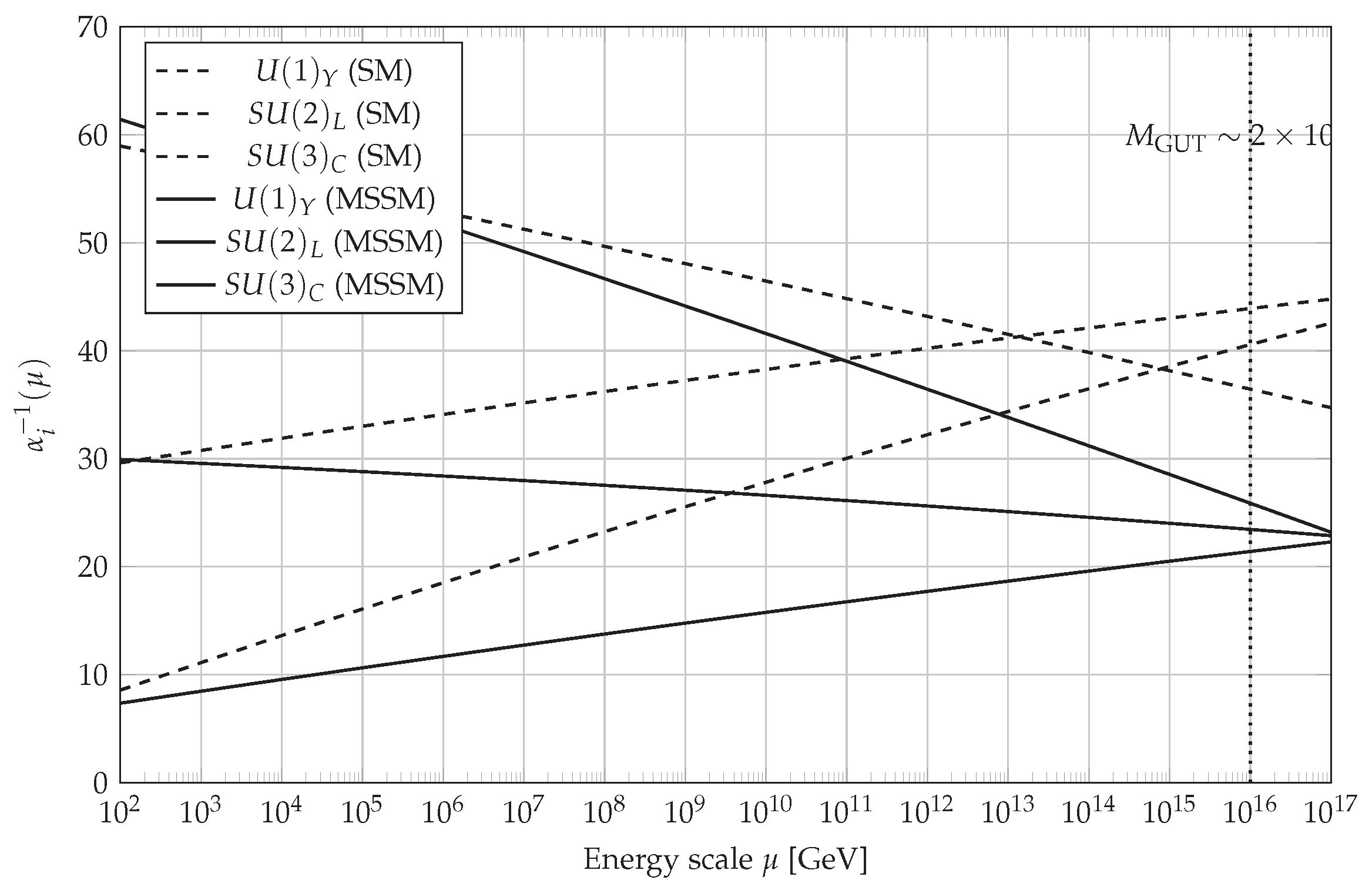
Extrapolating the measured gauge couplings to high energies using the RG equations, one finds that they do not unify exactly in the SM but approximately meet at a scale GeV if supersymmetry is included [41,42]. This observation is a key hint for grand unification (Section 11.1).
Figure 3.
Two-loop renormalization group evolution of the inverse gauge couplings in the Standard Model and the Minimal Supersymmetric Standard Model. The figure shows the running of the GUT-normalized inverse couplings for , , and from the electroweak scale up to . The dashed curves correspond to the Standard Model evolution using the one-loop beta coefficients supplemented by leading two-loop corrections encoded in the matrix , which generate the mild curvature visible in the trajectories. The solid curves represent the Minimal Supersymmetric Standard Model (MSSM), where the modified particle content above the supersymmetry threshold (assumed here at ) alters the beta-function coefficients to and correspondingly modifies the two-loop contributions. In the non-supersymmetric case, the three couplings fail to intersect at a common point, demonstrating the absence of exact gauge unification within the minimal Standard Model. In contrast, the supersymmetric evolution yields near-convergence at , a central theoretical motivation for supersymmetric Grand Unified Theories. The logarithmic horizontal axis emphasizes the vast hierarchy between the electroweak scale and the unification scale, spanning approximately fourteen orders of magnitude in energy.
8.3. Higgs Mass and Vacuum Stability
8.4. Radiative Corrections to Masses
The Higgs mass receives quadratically divergent corrections from loops, leading to the hierarchy problem: why is so much smaller than the Planck scale? In the SM, these corrections must be fine-tuned to cancel. This unnatural fine-tuning motivates supersymmetry (Section 11.2), where the divergences cancel between particles and superpartners.
9. Gravity and the Standard Model
Gravity is not included in the SM. At low energies, it can be described by the Einstein-Hilbert action
where is Newton’s constant and R the Ricci scalar. When quantized as an effective field theory, gravity becomes non-renormalizable: an infinite number of counterterms are needed to absorb divergences at loop level [67]. This suggests that a more fundamental theory (e.g., string theory) is required at the Planck scale GeV.
Coupling the SM to gravity in a consistent manner is an open problem. Approaches include effective field theory, asymptotic safety, and ultraviolet completions such as string theory (Section 11.5).
10. Experimental Milestones and Precision Tests
The SM has been tested with remarkable precision across many energy scales. Here we summarize key experimental confirmations and the ongoing search for deviations.
10.1. Discovery of the W and Z Bosons
The and Z bosons were discovered in 1983 by the UA1 and UA2 collaborations at CERN’s collider [51,52]. Their masses were measured to be GeV and GeV, in excellent agreement with SM predictions. This confirmed the electroweak unification and the Higgs mechanism (though the Higgs itself was not yet found).
10.2. Top Quark Discovery
10.3. Neutrino Oscillations
The discovery of neutrino oscillations by Super-Kamiokande (atmospheric neutrinos) in 1998 [49] and SNO (solar neutrinos) in 2001 [50] provided the first definitive evidence for physics beyond the minimal SM. Neutrinos have mass, and they mix. Subsequent experiments (KamLAND, MINOS, Daya Bay, T2K, NOvA) have measured the oscillation parameters with increasing precision [10].
10.4. Higgs Boson Discovery
On July 4, 2012, the ATLAS and CMS collaborations announced the discovery of a new particle with mass around 125 GeV, consistent with the SM Higgs boson [55,56]. Subsequent measurements have confirmed its spin-parity and couplings to gauge bosons and fermions, in agreement with SM expectations within current uncertainties.
10.5. Precision Electroweak Tests
Experiments at LEP (CERN), SLC (SLAC), and the Tevatron have measured numerous observables (e.g., Z pole parameters, W mass, forward-backward asymmetries) with high precision. Global fits to SM parameters show remarkable consistency [10]. For example, the top quark mass predicted from electroweak data before its discovery agreed well with the measured value.
10.6. Direct Searches for New Physics
The LHC continues to search for new particles predicted by BSM theories, such as supersymmetric partners, extra gauge bosons, and dark matter candidates. So far, no unambiguous signals have been found, placing stringent limits on the masses of such particles (e.g., gluinos > 2 TeV, squarks > 1 TeV) [68,69].
11. Beyond the Standard Model
Despite its successes, the SM leaves many questions unanswered. Here we discuss prominent extensions addressing these issues.
11.1. Grand Unified Theories (GUTs)
Grand Unified Theories embed into a larger simple group, unifying the strong and electroweak interactions at a high scale GeV. The simplest example is [38], where one generation fits into representations. predicts relations among fermion masses (e.g., at the GUT scale) and proton decay via . The non-observation of proton decay (lifetime years) rules out minimal non-supersymmetric but allows supersymmetric versions [41,44].
11.2. Supersymmetry (SUSY)
Supersymmetry relates bosons and fermions, introducing superpartners for all SM particles. The Minimal Supersymmetric Standard Model (MSSM) [41,42,43] has several attractive features: it stabilizes the Higgs mass against quadratic divergences (solving the hierarchy problem), provides a dark matter candidate (the lightest neutralino if R-parity is conserved), and improves gauge coupling unification. The predicted superpartner masses, however, have not been found, pushing the scale of SUSY breaking above the TeV range in many models.
11.3. Seesaw Mechanism and Neutrino Mass
The seesaw mechanism explains the smallness of neutrino masses by introducing heavy right-handed neutrinos with Majorana masses. The Lagrangian includes
11.4. Dark Matter Candidates
Astrophysical and cosmological evidence strongly suggests that about 85% of the matter in the universe is non-luminous dark matter [57]. The SM provides no viable candidate. Popular BSM candidates include:
- Weakly Interacting Massive Particles (WIMPs), such as the lightest neutralino in SUSY.
- Axions, arising from the Peccei-Quinn solution to the strong CP problem.
- Sterile neutrinos (right-handed neutrinos with keV-scale masses).
- Primordial black holes (though constraints are severe).
Direct detection experiments (XENON, LUX, PandaX) and indirect searches (Fermi-LAT, AMS-02) are actively hunting for these particles [58].
11.5. String Theory and Quantum Gravity
String theory provides a consistent framework for quantum gravity and naturally unifies all interactions. In string constructions, the SM gauge group and matter content can emerge from compactifications of extra dimensions (e.g., heterotic on Calabi-Yau manifolds, intersecting brane models) [60,61]. String theory also predicts supersymmetry and often contains GUT structures. While direct tests are far beyond current capabilities, string-inspired phenomenology (e.g., low-energy effective actions, moduli fields) offers connections to observable physics.
11.6. Baryogenesis and Leptogenesis
The observed baryon asymmetry of the universe requires three Sakharov conditions [59]: baryon number violation, C and CP violation, and departure from thermal equilibrium. The SM fails to generate enough CP violation and lacks sufficient baryon number violation. In leptogenesis [59], the out-of-equilibrium decay of heavy right-handed neutrinos generates a lepton asymmetry, which is then converted to a baryon asymmetry by sphaleron processes. This mechanism ties the seesaw scale to the observed asymmetry.
12. Conclusion and Outlook
The Standard Model Lagrangian, as derived and dissected in this review, provides a comprehensive and extraordinarily successful description of particle physics up to the electroweak scale. Its gauge structure, spontaneous symmetry breaking, and renormalizability have been confirmed by decades of precision experiments. The discovery of the Higgs boson in 2012 crowned this achievement.
Nevertheless, the SM is incomplete. It leaves fundamental questions unanswered: the origin of fermion masses and mixings, the nature of dark matter, the baryon asymmetry, the strong CP problem, and the inclusion of gravity. These open problems drive an intense experimental and theoretical program. The LHC continues to explore the TeV scale, searching for new particles and interactions. Neutrino experiments are refining our knowledge of oscillation parameters and searching for CP violation. Direct and indirect dark matter searches are pushing sensitivity limits. On the theory side, ideas such as grand unification, supersymmetry, extra dimensions, and string theory offer promising directions, though a complete, testable theory remains elusive.
The SM thus stands as both a triumph and a stepping stone. Its study has deepened our understanding of fundamental principles—gauge invariance, spontaneous symmetry breaking, renormalization—and will continue to guide us in the quest for a more unified description of nature.
Appendix A. Mathematical Supplements
Appendix A.1. Group Theory for the Standard Model
The SM gauge group is a direct product of simple and abelian factors. Representations are labeled by their dimensions under each factor and the charge. We summarize relevant properties:
Appendix A.1.1. SU(N) Fundamentals and Adjoints
For , the fundamental representation has dimension N, and the adjoint has dimension . Generators satisfy in the fundamental. Structure constants are defined by .
Appendix A.1.2. SU(2) and Pauli Matrices
For , generators in the fundamental are , with Pauli matrices. The adjoint representation is equivalent to the fundamental (since is pseudo-real). The structure constants are .
Appendix A.1.3. SU(3) and Gell-Mann Matrices
For , the eight generators in the fundamental are , where are Gell-Mann matrices. The adjoint representation has dimension 8, and the structure constants are tabulated in many references.
Appendix A.1.4. Hypercharge Assignments and Anomaly Cancellation
The hypercharge assignments in Table 1 are chosen to ensure that all gauge anomalies cancel. The condition for anomaly cancellation is , where the sum runs over all left-handed Weyl fermions. For one generation:
Similarly, the mixed anomaly requires , which we verified earlier.
Appendix A.2. Derivation of the Higgs Mechanism in Unitary Gauge
We provide a step-by-step derivation of gauge boson masses. Starting from the Higgs kinetic term:
Insert the VEV expansion . Compute each component:
Define and , with . Then
Thus,
The mass terms are read off as , with
Appendix A.3. One-Loop Beta Functions in the SM
References
- Peskin, M. E.; Schroeder, D. V. An Introduction to Quantum Field Theory; Addison-Wesley, 1995. [Google Scholar]
- S.Weinberg, The Quantum Theory of Fields, Vols. 1 and 2, Cambridge Univ. Press, 1995.
- Schwartz, M. D. Quantum Field Theory and the Standard Model; Cambridge Univ. Press, 2014. [Google Scholar]
- Halzen, F.; Martin, A. D. Quarks and Leptons: An Introductory Course in Modern Particle Physics; Wiley, 1984. [Google Scholar]
- Langacker, P. The Standard Model and Beyond, 2nd ed.; CRC Press, 2017. [Google Scholar]
- Nakahara, M. Geometry, Topology and Physics, 2nd ed.; CRC Press, 2003. [Google Scholar]
- Nash, C.; Sen, S. Topology and Geometry for Physicists; Academic Press, 1991. [Google Scholar]
- Bertlmann, R. A. Anomalies in Quantum Field Theory; Oxford Univ. Press, 1996. [Google Scholar]
- A. Bilal, "Lectures on Anomalies," arXiv:0802.0634 [hep-th]. arXiv:0802.0634.
- et al.; R. L. Workman et al. (Particle Data Group) Review of Particle Physics. Prog. Theor. Exp. Phys. 2022, 2022, 083C01. [Google Scholar] [CrossRef]
- Yang, C. N.; Mills, R. L. Conservation of Isotopic Spin and Isotopic Gauge Invariance. Phys. Rev. 1954, 96, 191. [Google Scholar] [CrossRef]
- Glashow, S. L. Partial-symmetries of weak interactions. Nucl. Phys. 1961, 22, 579. [Google Scholar] [CrossRef]
- Weinberg, S. A model of leptons. Phys. Rev. Lett. 1967, 19, 1264. [Google Scholar] [CrossRef]
- Salam, A. Elementary Particle Theory; Svartholm, N., Ed.; Almqvist and Wiksell, 1968. [Google Scholar]
- Higgs, P. W. Broken symmetries, massless particles and gauge fields. Phys. Lett. 1964, 12, 132. [Google Scholar] [CrossRef]
- Englert, F.; Brout, R. Broken symmetry and the mass of gauge vector mesons. Phys. Rev. Lett. 1964, 13, 321. [Google Scholar] [CrossRef]
- Guralnik, G. S.; Hagen, C. R.; Kibble, T. W. B. Global conservation laws and massless particles. Phys. Rev. Lett. 1964, 13, 585. [Google Scholar] [CrossRef]
- Goldstone, J. Field theories with Superconductor solutions. Nuovo Cim. 1961, 19, 154. [Google Scholar] [CrossRef]
- ’t Hooft, G.; Veltman, M. J. G. Regularization and renormalization of gauge fields. Nucl. Phys. B 1972, 44, 189. [Google Scholar] [CrossRef]
- Faddeev, L. D.; Popov, V. N. Feynman diagrams for the Yang-Mills field. Phys. Lett. B 1967, 25, 29. [Google Scholar] [CrossRef]
- Gross, D. J.; Wilczek, F. Ultraviolet Behavior of Non-Abelian Gauge Theories. Phys. Rev. Lett. 1973, 30, 1343. [Google Scholar] [CrossRef]
- Politzer, H. D. Reliable Perturbative Results for Strong Interactions? Phys. Rev. Lett. 1973, 30, 1346. [Google Scholar] [CrossRef]
- Fritzsch, H.; Gell-Mann, M.; Leutwyler, H. Advantages of the Color Octet Gluon Picture. Phys. Lett. B 1973, 47, 365. [Google Scholar] [CrossRef]
- Cabibbo, N. Unitary symmetry and leptonic decays. Phys. Rev. Lett. 1963, 10, 531. [Google Scholar] [CrossRef]
- Kobayashi, M.; Maskawa, T. CP-violation in the renormalizable theory of weak interaction. Prog. Theor. Phys. 1973, 49, 652. [Google Scholar] [CrossRef]
- Pontecorvo, B. Mesonium and anti-mesonium. Sov. Phys. JETP 1957, 6, 429. [Google Scholar]
- Maki, Z.; Nakagawa, M.; Sakata, S. Remarks on the unified model of elementary particles. Prog. Theor. Phys. 1962, 28, 870. [Google Scholar] [CrossRef]
- Adler, S. L. Axial vector vertex in spinor electrodynamics. Phys. Rev. 1969, 177, 2426. [Google Scholar] [CrossRef]
- Bell, J. S.; Jackiw, R. A PCAC puzzle: pi0 to gamma gamma in the sigma model. Nuovo Cim. A 1969, 60, 47. [Google Scholar] [CrossRef]
- Peccei, R. D.; Quinn, H. R. CP Conservation in the Presence of Pseudoparticles. Phys. Rev. Lett. 1977, 38, 1440. [Google Scholar] [CrossRef]
- Weinberg, S. A New Light Boson? Phys. Rev. Lett. 1978, 40, 223. [Google Scholar] [CrossRef]
- Wilczek, F. Problem of Strong P and T Invariance in the Presence of Instantons. Phys. Rev. Lett. 1978, 40, 279. [Google Scholar] [CrossRef]
- Nambu, Y.; Jona-Lasinio, G. Dynamical Model of Elementary Particles Based on an Analogy with Superconductivity. I. Phys. Rev. 1961, 122, 345. [Google Scholar] [CrossRef]
- Lee, B. W.; Quigg, C.; Thacker, H. B. Weak interactions at very high energies: The role of the Higgs-boson mass. Phys. Rev. D 1977, 16, 1519. [Google Scholar] [CrossRef]
- Ford, C.; Jack, I.; Jones, D. R. T. The Standard model effective potential at two loops. Nucl. Phys. B 1993, 395, 17. [Google Scholar] [CrossRef]
- Buttazzo, D. Investigating the near-criticality of the Higgs boson. JHEP 2013, arXiv:1307.353612, 089. [Google Scholar] [CrossRef]
- de Gouvêa, A. Vacuum stability and the Higgs boson. Phys. Rev. D 2014, arXiv:1403.555889, 115012. [Google Scholar]
- Georgi, H.; Glashow, S. L. Unity of All Elementary-Particle Forces. Phys. Rev. Lett. 1974, 32, 438. [Google Scholar] [CrossRef]
- Fritzsch, H.; Minkowski, P. Unified Interactions of Leptons and Hadrons. Annals Phys. 1975, 93, 193. [Google Scholar] [CrossRef]
- Georgi, H. , in Particles and Fields (AIP, 1975).
- Dimopoulos, S.; Georgi, H. Softly Broken Supersymmetry and SU(5). Nucl. Phys. B 1981, 193, 150. [Google Scholar] [CrossRef]
- Ibanez, L. E.; Ross, G. G. Low-Energy Predictions in Supersymmetric Grand Unified Theories. Phys. Lett. B 1981, 105, 439. [Google Scholar] [CrossRef]
- S. P. Martin, "A Supersymmetry Primer," Adv. Ser. Direct. High Energy Phys. 18, 1 (1998) [hep-ph/9709356].
- Sakai, N. Proton Decay in Supersymmetric GUTs. Z. Phys. C 1981, 11, 153. [Google Scholar] [CrossRef]
- Minkowski, P. μ→eγ at a Rate of One Out of 109 Muon Decays? Phys. Lett. B 1977, 67, 421. [Google Scholar] [CrossRef]
- Yanagida, T. Horizontal Symmetry and Masses of Neutrinos. Prog. Theor. Phys. in Japanese. 1980, 64, 1103. [Google Scholar] [CrossRef]
- Glashow, S. L. The Future of Elementary Particle Physics, in Quarks and Leptons; Plenum, 1980. [Google Scholar]
- Mohapatra, R. N.; Senjanović, G. Neutrino Mass and Spontaneous Parity Violation. Phys. Rev. Lett. 1980, 44, 912. [Google Scholar] [CrossRef]
- Fukuda, Y.; et al. Evidence for oscillation of atmospheric neutrinos. Phys. Rev. Lett. 1998, 81, 1562. [Google Scholar] [CrossRef]
- Ahmad, Q. R.; et al. Measurement of the Rate of νe+d→p+p+e- Interactions Produced by 8B Solar Neutrinos at the Sudbury Neutrino Observatory. Phys. Rev. Lett. 2001, 87, 071301. [Google Scholar] [CrossRef]
- Arnison, G.; et al. Experimental observation of isolated large transverse energy electrons with associated missing energy at s=540 GeV. Phys. Lett. B 1983, 122, 103. [Google Scholar] [CrossRef]
- Banner, M.; et al. Observation of single isolated electrons of high transverse momentum in events with missing transverse energy at the CERN p¯p collider. Phys. Lett. B 1983, 122, 476. [Google Scholar] [CrossRef]
- Abachi, S.; et al. Observation of the Top Quark. Phys. Rev. Lett. 1995, 74, 2632. [Google Scholar] [CrossRef]
- Abe, F.; et al. Observation of Top Quark Production in p¯p Collisions. Phys. Rev. Lett. 1995, 74, 2626. [Google Scholar] [CrossRef]
- ATLAS Collaboration (G. Aad et al.), "Observation of a new particle in the search for the Standard Model Higgs boson with the ATLAS detector at the LHC," Phys. Lett. B 716, 1 (2012).
- Chatrchyan, S.; CMS Collaboration. Observation of a new boson at a mass of 125 GeV with the CMS experiment at the LHC. Phys. Lett. B 2012, 716, 30. [Google Scholar] [CrossRef]
- Aghanim, N.; Planck Collaboration. Planck 2018 results. VI. Cosmological parameters. Astron. Astrophys. 2020, arXiv:1807.06209641, A6. [Google Scholar]
- Bertone, G.; Hooper, D.; Silk, J. Particle dark matter: evidence, candidates and constraints. Phys. Rept 2005, 405, 279. [Google Scholar] [CrossRef]
- Sakharov, A. D. Violation of CP Invariance, C Asymmetry, and Baryon Asymmetry of the Universe. Pisma Zh. Eksp. Teor. Fiz. 1967, 5, 32. [Google Scholar]
- Polchinski, J. String Theory, Vols. 1–2; Cambridge Univ. Press, 1998. [Google Scholar]
- Green, M. B.; Schwarz, J. H.; Witten, E. Superstring Theory; Cambridge Univ. Press, 1987; Vols. 1–2. [Google Scholar]
- Amaldi, U.; de Boer, W.; Fürstenau, H. Comparison of grand unified theories with electroweak and strong coupling constants measured at LEP. Phys. Lett. B 1991, 260, 447. [Google Scholar] [CrossRef]
- Feynman, R. P. Quantum Electrodynamics; Benjamin, 1961. [Google Scholar]
- Schwinger, J. Selected Papers on Quantum Electrodynamics; Dover, 1958. [Google Scholar]
- Lee, T. D.; Yang, C. N. Question of Parity Conservation in Weak Interactions. Phys. Rev. 1956, 104, 254. [Google Scholar] [CrossRef]
- Wu, C. S. Experimental Test of Parity Conservation in Beta Decay. Phys. Rev. 1957, 105, 1413. [Google Scholar] [CrossRef]
- Weinberg, S. Ultraviolet divergences in quantum theories of gravitation. In General Relativity: An Einstein Centenary Survey; Hawking, S. W., Israel, W., Eds.; Cambridge Univ. Press, 1979. [Google Scholar]
- ATLAS Collaboration. "SUSY searches" (latest results). Available online: https://twiki.cern.ch/twiki/bin/view/AtlasPublic/SupersymmetryPublicResults.
- CMS Collaboration. "SUSY searches" (latest results). Available online: https://twiki.cern.ch/twiki/bin/view/CMSPublic/PhysicsResultsSUS.
Figure 1.
Three-gluon vertex arising from the non-abelian interaction.
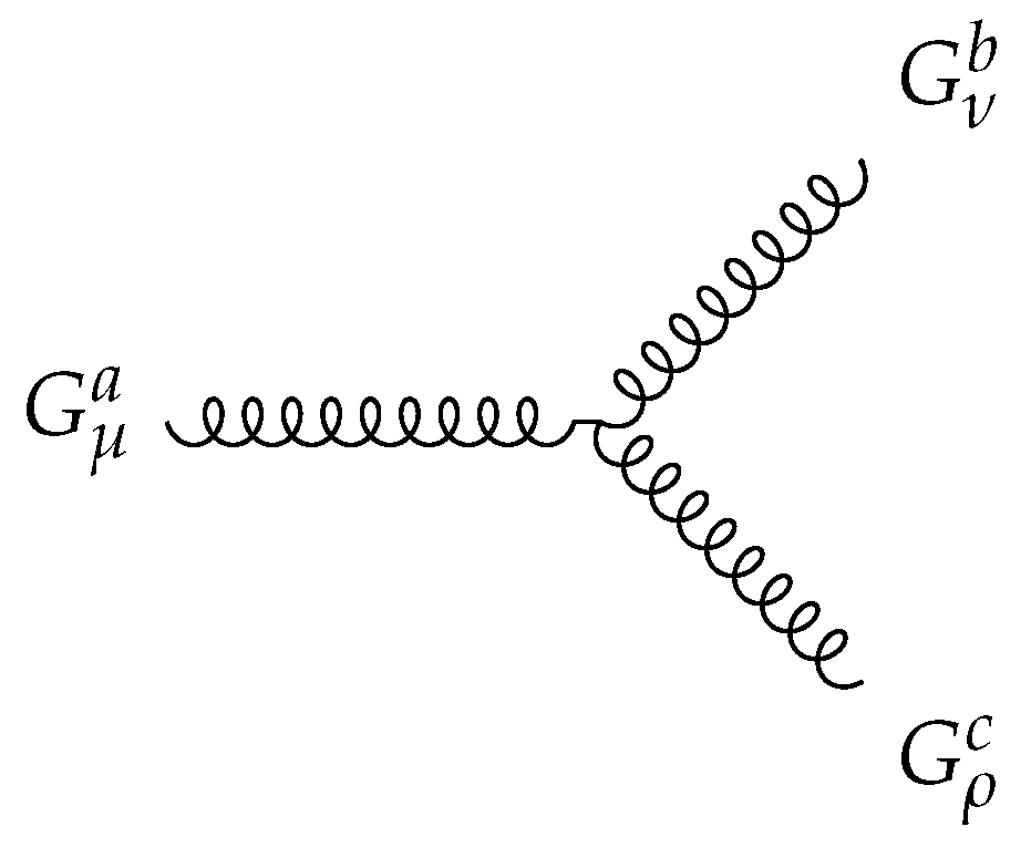
Figure 2.
Four-gluon vertex from the interaction.
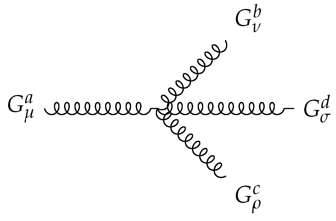

Table 1.
Fermion multiplets of one generation in the SM. The subscript L denotes left-handed chirality, and R right-handed. Hypercharge assignments are fixed by the relation .
Table 1.
Fermion multiplets of one generation in the SM. The subscript L denotes left-handed chirality, and R right-handed. Hypercharge assignments are fixed by the relation .
| Field | Representation | Y | Electric Charge Q |
|---|---|---|---|
Disclaimer/Publisher’s Note: The statements, opinions and data contained in all publications are solely those of the individual author(s) and contributor(s) and not of MDPI and/or the editor(s). MDPI and/or the editor(s) disclaim responsibility for any injury to people or property resulting from any ideas, methods, instructions or products referred to in the content. |
© 2026 by the authors. Licensee MDPI, Basel, Switzerland. This article is an open access article distributed under the terms and conditions of the Creative Commons Attribution (CC BY) license (http://creativecommons.org/licenses/by/4.0/).
Copyright: This open access article is published under a Creative Commons CC BY 4.0 license, which permit the free download, distribution, and reuse, provided that the author and preprint are cited in any reuse.


