
Submitted:
26 February 2026
Posted:
27 February 2026
You are already at the latest version
Abstract
Accurate characterization and structured interpretation of qubit errors are essential for advancing scalable quantum computation. In this work, we introduce a Category-Based Error Budgeting ($CBEB$) framework for systematic analysis of qubit calibration data in noisy intermediate-scale quantum ($NISQ$) processors. The proposed methodology decomposes the total error budget into physically and statistically meaningful categories, enabling quantitative evaluation of their relative contributions through two core metrics: the relative contribution rate ( $R_A$ ) and the disproportionality factor ( $D_A$).Beyond static categorization, the framework incorporates correlation-aware analysis by constructing covariance structures derived from two-qubit gate errors, allowing error interdependencies to be explicitly modeled. We further integrate the budgeting formalism into decoder weight assignment strategies and compare three decoding models: uniform weighting, individual error-based weighting, and a category-correlation-aware model. Logical error rates are estimated under each scheme to evaluate performance impact.The framework is implemented as an interactive graphical analysis tool and validated using real calibration datasets from contemporary superconducting quantum processors. Results demonstrate that category-level decomposition reveals structurally dominant error sources that are not evident from aggregate statistics alone, and that correlation-aware weighting provides improved logical error rate estimation.This work establishes a principled and operational bridge between calibration diagnostics and decoder optimization, offering a scalable methodology for structured error analysis in near-term quantum hardware.
Keywords:
quantum error correction
; error budgeting
; Qubit Classification
; quantum processor characterization
; heterogeneous noise
1. Introduction and Motivation
1.1. The Measurement Error Challenge in Quantum Computing
Quantum measurement represents the critical point when relating a sample of probabilistic results obtained from quantum states to classical systems. Unlike classical measurements, which produce deterministic values, quantum measurement is inherently probabilistic and is affected by multiple noise sources, such as electromagnetic, thermal, and quantum entanglement effects, among others. Beyond technical limitations, quantum measurement introduces fundamental perturbations in quantum states, which can lead to logical errors that directly impact computational reliability.
Importantly, measurement (readout) errors are governed by physical mechanisms fundamentally different from those responsible for gate operations. Consequently, readout error rates are generally not proportional to gate error rates, i.e., . This chapter invalidates the assumptions of uniform noise and underscores the need for independent frameworks for measurement error budgeting.
1.2. Gap in Existing Characterization Methodologies
Current quantum hardware characterization operates at two distinct levels: fine-grained qubit-level metrics and coarse-grained device-level statistical indicators. Both approaches lack structured frameworks to characterize collective effects of correlated qubit subsets or analyze fractional contributions of different error sources within total error budgets. This methodological gap becomes increasingly significant as quantum processors scale to hundreds of qubits, where spatial and temporal heterogeneity cannot be ignored.
1.3. Our Contribution: A Comprehensive Framework
This work introduces a comprehensive category-based framework for measurement error budgeting that: (1) quantifies heterogeneity through novel metrics, (2) enables actionable diagnostics for critical qubit identification, (3) bridges to error correction through decoder-aware formulations, (4) accounts for spatial and temporal correlations, and (5) provides practical algorithms for error-aware resource allocation in both NISQ and fault-tolerant quantum computing.
2. Theoretical Framework for Quantum Measurement Noise
2.1. Probabilistic Models of Measurement Noise
2.1.1. Response Matrices and Conditional Error Rates
For each qubit i, the measurement process can be described by a response matrix :
where is the probability of measuring outcome b given the true state a. The readout error rate is then:
For multi-qubit systems, the full response matrix grows exponentially, necessitating efficient approximations.
2.1.2. Correlated Noise Models
In practice, measurement errors are often correlated due to shared control lines, crosstalk, and environmental fluctuations. A general correlated noise model can be expressed as:
where is the independent error model, are correlation strengths, and capture pairwise correlations [1].
2.2. Impact of Measurement Noise on Quantum Algorithms
2.2.1. Effect on NISQ Applications
For Noisy Intermediate-Scale Quantum (NISQ) applications, measurement errors directly affect algorithm success probabilities. The expected output distribution becomes:
where is the ideal output distribution. This distortion can significantly impact variational algorithms, quantum simulation, and other NISQ applications [2].
2.2.2. Implications for Fault-Tolerant Computing
In fault-tolerant quantum computing, measurement errors affect syndrome extraction for quantum error correction. The effective error rate for a distance-d surface code under measurement noise is:
where is the threshold and is the effective measurement error rate [3].
2.3. Limitations of Current Noise Models
2.3.1. Assumption of Statistical Independence
Most existing models assume independent errors across qubits, neglecting spatial correlations that are prevalent in large-scale processors [8].
2.3.2. Neglect of Temporal Variations
Static error models fail to capture time-dependent fluctuations due to calibration drift, environmental changes, and device aging [12].
2.3.3. Uniformity Assumptions
Homogeneous noise models ignore the significant spatial heterogeneity observed in experimental devices, leading to suboptimal error correction and resource allocation.
3. Historical Development of Qubit Classification Methodologies
3.1. Foundations and the Experimental Era (2000–2010)
3.1.1. From Demonstrations to Quantum Standards
The first decade of experimental quantum computing witnessed a shift from verifying fundamental quantum phenomena to establishing comprehensive performance standards. Early work in the late 1990s and early 2000s within nuclear magnetic resonance and trapped ion systems confirmed core concepts such as superposition and entanglement [13,14]. Concurrently, pioneering work in superconducting circuits established metrics like coherence times (, ), gate fidelities, and readout fidelities [15] as comparable benchmarks for the field.
3.1.2. The Emergence of Multidimensional Measurements
DiCarlo et al. (2009) exemplified a maturing performance measurement methodology, combining multiple metrics to assess the implementation of quantum algorithms on superconducting processors [16]. This work demonstrated that functional quantum processors require consistent, synchronized performance across multiple independent metrics—not merely a binary success criterion. High-fidelity gates alone are insufficient, and long coherence times are not enough; high-fidelity readout is equally critical.
3.2. The Era of Scaling and Complexity (2010–2018)
3.2.1. Classification Based on Individual Performance Metrics
With systems scaling from 5 to 20 qubits, classification evolved to encompass various independent metrics: single- and two-qubit gate errors, coherence times (, ), and readout fidelity. While providing a multidimensional characterization, these metrics lacked systematic aggregation into a unified framework [17]. Performance classification during this period was often ad hoc, with no standardized method for synthesizing these disparate measures into a single, comprehensive score for direct platform comparison.
3.2.2. Cluster-Based Methodologies
Murali et al. (2019) applied clustering techniques to qubits, treating the performance data of each qubit as an independent dataset [18]. Their focus was on leveraging noise profiles (e.g., error rates, coherence times) to guide more efficient compilation and mapping of quantum programs, thereby improving execution success rates on NISQ devices. Linke et al. (2017), in a comparative study of device architectures, demonstrated that differences in algorithm performance are intrinsically linked to structural properties such as qubit connectivity and physical layout [19].
3.2.3. Spatial Classification Methods
Research has indicated significant performance variation among qubits within superconducting devices based on their physical location within the chip architecture. Studies of energy relaxation time fluctuations have revealed that spatial position is an implicit factor influencing error rates and coherence properties, reflecting the manufacturing and control challenges inherent in multi-qubit NISQ processor design [20].
3.2.4. Algorithm-Conscious Classification
As quantum applications diversified in the NISQ era, researchers began exploring methodologies that explicitly link algorithm requirements to device properties to optimize qubit mapping. This approach, often termed algorithm-aware or application-oriented mapping, considers factors like coherence times, error rates, and inter-qubit connectivity to enhance the executability and success rate of specific algorithms compared to naive allocation methods [21].
3.2.5. Dynamic Classification Methodologies
The temporal instability of device characteristics and its impact on algorithm performance has also been addressed. Studies using direct randomized benchmarking suggest that drifts in error rates and noise patterns over time can degrade classification quality and map suitability, necessitating dynamic methodologies to monitor and systematically adapt to this temporal variability [12].
3.3. The Contemporary Era (2022–Present): Towards Comprehensive Performance Metrics
3.3.1. From Individual Physical Measures to Integrated Standards
The contemporary era is marked by a decisive shift from reliance on isolated physical measures (e.g., coherence times, gate fidelities) towards integrated, system-level benchmarks. These benchmarks aim to provide a more holistic and realistic characterization of overall quantum processor capability. Prominent among these are:
- Quantum Volume (QV): A holistic metric that combines usable qubit count, gate fidelity, and executable circuit depth to benchmark a processor’s ability to run general, random circuits [22].
- Circuit Layer Operations Per Second (CLOPS): A metric focusing on computational throughput, measuring the execution rate of quantum circuit layers while accounting for classical control, reset, and readout operations [23].
- Algorithmic Qubits (AQ): An application-oriented metric that evaluates processor performance on specific, commercially relevant algorithms rather than random circuits, reflecting the industry’s shift towards benchmarking for practical utility [24].
These metrics reflect a general trend towards evaluating quantum processors as integrated systems, rather than as a simple sum of their parts.
3.3.2. Comprehensive Performance Classification
Modern trends in qubit and quantum processor performance classification advocate for a holistic approach that transcends localized characterization, incorporating:
- Architectural characteristics, such as qubit connectivity topology and crosstalk profiles.
- Explicit correlations between low-level physical metrics (noise, coherence) and application-level algorithmic outcomes.
- Integration of performance temporal stability into the evaluation framework, acknowledging the observed fluctuations in NISQ device parameters over time [12].

Table 1.
Comparison of Qubit Classification Methodologies
| Methodology | Advantages | Limitations | Suitable Domains |
|---|---|---|---|
| Binary Classification | Simplicity of implementation; fast evaluation | Oversimplification; ignores inter-qubit variance | Early-stage prototypes |
| Multi-class Classification | Higher accuracy; better characterization of variance | Computational complexity; sensitivity to threshold selection | Medium-scale systems |
| Dynamic Classification | Adapts to time-dependent performance drifts | Requires continuous calibration data and monitoring infrastructure | Long-term operational systems |
| Proposed Framework | Comprehensive, quantitative, and application-aware | Requires accurate calibration and real-time monitoring | Advanced QC; scalable systems |
4. Our Category-Based Error Budgeting Framework
4.1. Contributions to Classification Methodology
4.1.1. Methodological Innovations
1. Budget-based Classification: Focuses on relative contribution to total system error budget rather than absolute performance, identifying critical qubits with disproportionate system impact.
2. Multi-scale Classification: Hierarchical approach analyzing individual qubits, category aggregation, and system-level interactions.
3. Context-aware Classification: Incorporates algorithmic, hardware, and correction contexts to improve upon static methodologies [5].
4.1.2. Integration with Previous Methodologies
Our framework complements and extends previous approaches by:
- Integrating with IBM’s metric-based individual characterization
- Extending spatial classification with quantitative impact analysis
- Adding temporal dimension to hybrid classification approaches
- Providing bridging between classification and error correction requirements
4.2. Theoretical Foundations
4.2.1. Core Theoretical Claim
Claim: Incorporating category-resolved and correlation-weighted measurement errors into decoder weights provides strictly more informative noise representation for fault-tolerant decoders than uniform or spatially-averaged error models, given fixed calibration information.
The primary objective of this work is the development of a theoretical error classification and budgeting framework. Experimental data are used only to provide illustrative instantiations of selected components of the framework, subject to data availability.
Formalized as information-theoretic claim:
where I represents mutual information between noise models and optimal decoder weights [7].
4.2.2. Qubit-Specific Measurement Error Rates
We begin by considering measurement-layer observables, as these are universally available across current quantum hardware platforms.
For each qubit , define measurement error rate:
Statistical averages from calibration experiments:
4.2.3. Total Expected Measurement Error
Define total measurement error budget:
Modeling assumptions: First-order additivity, statistical independence, time-invariance (explicitly relaxed in extensions).
4.2.4. Category-Based Partitioning
Partition qubit set into disjoint categories:
where is category labels set.
Table 2.
Category Definition Criteria.
| Criteria | Definition Method | Typical Applications |
|---|---|---|
| Spatial Layout | Physical location on processor chip | Thermal gradient analysis, crosstalk mapping |
| Coherence Properties | , , dephasing rates | Coherence-limited algorithm mapping |
| Hardware Zones | Shared control/readout electronics | Resource contention optimization |
| Gate Fidelity Classes | CNOT error rates, single-qubit gate errors | Gate-aware compilation |
| Error Rate Thresholds | Empirical error rate bins | Error mitigation strategy selection |
4.2.5. Category Error Sums and Fractional Contributions
For category :
Central diagnostic quantity:
Normalized per-qubit contribution and disproportionality factor:
indicates category A contributes more than its fair share per qubit.
4.2.6. New Classification Metrics
We introduce quantitative metrics advancing classification methodology:
5. Advanced Extensions and Generalizations
5.1. From Relative to Absolute Error Rates
Given total physical error rate , define category-level absolute rates:
Here, should be interpreted as an effective measurement-induced physical error rate relevant to syndrome extraction, rather than a gate-level error rate.
5.2. Correlated Noise Modeling: Covariance Matrix Extension
To capture correlated readout noise effects observed in multi-qubit devices [6,8], we extend our model by introducing a covariance matrix :
where is the readout error of qubit i in the k-th calibration shot, is the mean error rate, and M is the total number of calibration measurements.
The correlated total error rate is then expressed as:
For category-level analysis:
5.3. Temporal Dynamics and Non-Stationary Errors
Real quantum devices exhibit time-varying error rates due to environmental fluctuations, calibration drift, and aging effects [9,10]. We model this temporal behavior as:
The time-averaged category contribution over interval T is:
Temporal correlations with time lag :
5.4. Algorithm-Specific Category Analysis
To validate the algorithm-aware extension of our theoretical framework, we select representative quantum algorithms from different application domains:
- Algorithm A (Circuit-Heavy): A deep random circuit benchmark (e.g., Quantum Volume circuit) with high two-qubit gate density.
- Algorithm B (Measurement-Heavy): A variational quantum eigensolver (VQE) for a small molecule, with repeated state preparation and measurement.
- Algorithm C (Memory-Dominated): A dynamical decoupling or idle benchmarking sequence.
For each algorithm , we:
- Analyze the circuit to compute qubit usage frequencies and gate-type frequencies .
- Calculate algorithm-specific category contributions using:
- Compare these algorithm-specific rankings with the static category contributions to identify cases where qubit importance shifts significantly based on algorithmic context.
6. Decoder-Aware Formulation and Fault-Tolerance Integratio
6.1. Position in the Fault-Tolerance Pipeline
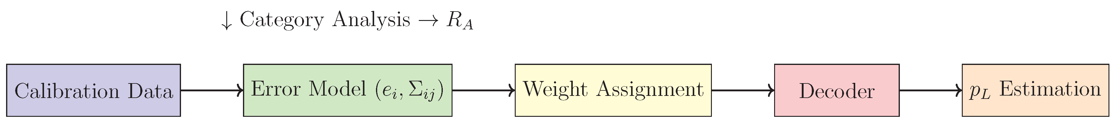
Our work occupies a position in the fault-tolerant quantum computing stack, serving as the bridge between device calibration and decoder implementation.
Figure 1.
Our approach takes raw calibration data, extracts correlated error models, assigns decoder-aware weights, and enables accurate logical error rate estimation.
Figure 1.
Our approach takes raw calibration data, extracts correlated error models, assigns decoder-aware weights, and enables accurate logical error rate estimation.
6.2. Weight Assignment for Minimum-Weight Perfect Matching Decoders
6.3. Logical Error Rate Estimation with Heterogeneous Noise
With category-aware weights, the logical error rate for a distance-d code:
The category disproportionality factor directly influences logical performance:
6.4. Integration with Union-Find and Other Decoders
For Union-Find decoders [11], we define qubit-level erasure probabilities:
where is an amplification factor, and controls correlation contribution.
7. Experimental Procedures: Proposed Implementation of Theoretical Framework
This section outlines the concrete, hardware-agnostic experimental procedures for implementing and validating the theoretical category-based error budgeting framework presented in the main text. The steps are described sequentially, providing a roadmap for experimental verification without presenting results.
7.1. Experimental Setup and Initial Data Acquisition
-
Platform Selection and Access: Gain programmable access to a suitable superconducting, trapped-ion, or other quantum processing unit (QPU). Ensure the platform provides:
- Standard calibration data (readout error, , , gate errors).
- The ability to define and execute custom calibration circuits.
- (Ideally) access to time-series calibration data to test temporal extensions.
-
Baseline Calibration Data Collection: Execute standard characterization experiments for all N qubits to estimate:
- Individual qubit readout error rates, , via repeated preparation and measurement in the and states.
- For a subset of qubit pairs (especially those sharing readout resonators or control lines), perform correlated readout characterization. This involves preparing and measuring correlated two-qubit states (e.g., , ) to estimate the covariance matrix elements .
-
Definition of Theoretical Categories: Based on the hypothesis to be tested, define disjoint qubit categories using the processor’s metadata. Examples include:
- Spatial Classification: Group qubits by physical location on the chip (e.g., edge vs. center).
- Resource-Based Classification: Group qubits that share a common readout line, multiplexing resonator, or control channel.
- Error-Rate Classification: Partition qubits into low, medium, and high error rate bins based on initial measurements.
Record the category membership for each qubit, .
7.2. Implementation and Evaluation of Category-Based Budgeting
-
Calculation of Category Contributions: Apply the core theoretical formulas to the aggregated calibration data.
- Compute the total measurement error .
- For each category , calculate its error sum and its relative contribution rate .
- Compute the disproportionality factor .
-
Correlation-Aware Extension: Integrate the covariance data.
- Compute the correlation-corrected total error .
- Recalculate the category sums, separating internal and cross-category correlation contributions: .
- Recompute and using and .
-
Benchmarking Against Prior Classification Methods: Evaluate the differences in identifying critical qubits using:
- Our proposed category-budgeting method (ranking by or contribution to ).
- A simple threshold-based method (flagging all qubits with ).
- A pure spatial analysis (comparing average error rates of pre-defined zones).
7.3. Integration and Testing with Decoder-Aware Formulation
-
Construction of Weighted Error Models: For a target error-correcting code (e.g., a distance-3 surface code), generate a corresponding decoding graph. Assign weights to graph edges based on the underlying physical qubit error data.
- Uniform Model: Assign a constant weight
- Individual Model: For an edge associated with qubit i, assign
- Category-Correlation Model: Assignwhere is the neighborhood in the decoding graph and is a tunable parameter (initially set to 1).
-
Decoder Performance Comparison: Conduct simulated (or small-scale hardware) syndrome extraction experiments.
- Simulate the generation of syndrome data for the chosen code under a phenomenological noise model that incorporates the measured and, optionally, correlated jump events based on .
- Run the decoder (e.g., Minimum-Weight Perfect Matching or Union-Find) using the three different weight assignments defined above.
- Record the decoder’s success rate in identifying the correct error chain for each instance.
-
Logical Error Rate Estimation: Use the simulation outcomes to infer logical performance.
- For each weighting scheme, estimate the logical error rate by tallying the frequency of logical errors after correction.
- Compare
7.4. Validation of Theoretical Extensions
-
Temporal Dynamics Analysis: Collect time-series calibration data from the same QPU over an extended period (e.g., 24-48 hours, taking snapshots every 1-2 hours).
- For each time snapshot t, recompute , , and .
- Calculate the time-averaged category contribution and the Temporal Stability Index, .
- Compute the temporal correlation function for different time lags between snapshots.
-
Context-Sensitivity Testing: Execute calibration routines under different operational contexts.
- Context 1: Standard idle calibration.
- Context 2: Calibration preceded by high-intensity two-qubit gate operations on neighboring qubits (to induce potential crosstalk or heating).
- Context 3: Calibration using different readout pulse amplitudes or durations.
- For each context c, compute the context-dependent category contributions . Calculate the Context Sensitivity Metric, , for qubits that change category ranking across contexts.
7.5. Summary of Deliverables
- Category-to-Qubit Mapping Dataset: A comprehensive dataset mapping each qubit to its assigned category, accompanied by calculated category contribution rates and disproportionality factors . This validates the core budget-based classification methodology.
- Classification Method Comparison Matrix: A comparative matrix showing critical qubit sets identified by our proposed method versus baseline approaches (threshold-based, spatial-only, and uniform methods), demonstrating enhanced discriminative power.
- Decoder Performance Benchmarks: Quantitative decoder success rates and logical error probability estimates under different noise models (uniform, individual, and category-correlated), establishing the practical utility of our framework for fault-tolerant protocols.
- Temporal Evolution Visualizations: Time-series plots tracking over extended periods, along with temporal correlation functions , validating the framework’s ability to capture non-stationary device behavior.
- Context Sensitivity Quantification: Numerical values of the Context Sensitivity Metric for qubits exhibiting significant performance variation across different operational contexts, demonstrating the necessity of context-aware classification.
8. Analysis of Qubit Calibration Results for IBM Boston – 19 February 2026
Performance Analysis Report of the IBM Boston Quantum Processor
Calibration Date: 19 February 2026
Analysis Date: 22 February 2026
8.1. Executive Summary
Calibration data from 156 qubits of the IBM Boston quantum processor were analyzed using the Category-Based Error Budgeting methodology. The objective was to evaluate qubit performance and quantify heterogeneous error contributions across the device.
The results reveal substantial variability in qubit performance. Readout errors range from 0.00098 to 0.2585, with a mean value of 0.00965.
Key Findings:
- Total error budget (): 1.505362
- Correlation-aware total error (): 3.449852 (129% increase relative to )
- Number of two-qubit gates: 352
-
Most disproportionate categories:
- -
- Very_High_Error ()
- -
- Very_Low_Coherence ()
8.2. Applied Methodology
Step 7.1 – Data Collection
Calibration data were imported from an Excel file and cleaned prior to analysis. The dataset included:
- Single-qubit parameters: , , readout error, single-qubit gate errors
- Two-qubit gate data: CZ errors, RZZ errors, gate durations
- Connectivity information: 352 coupled qubit pairs
Step 7.2 – Qubit Classification
Three classification schemes were applied.
(A) Spatial Classification
- A_Low_Range (0–49): 50 qubits
- B_Mid_Range (50–99): 50 qubits
- C_High_Range (100–129): 30 qubits
- D_Very_High_Range (130–155): 26 qubits
(B) Error-Rate Classification
Based on readout error:
- Low_Error (): 75 qubits (48%)
- Medium_Error (0.005–0.01): 57 qubits (36.5%)
- High_Error (0.01–0.02): 18 qubits (11.5%)
- Very_High_Error (): 6 qubits (4%)
(C) Coherence Classification
Based on average coherence time (, ):
- High_Coherence (): 84 qubits (54%)
- Medium_Coherence (200–300 ): 55 qubits (35%)
- Low_Coherence (100–200 ): 9 qubits (6%)
- Very_Low_Coherence (): 8 qubits (5%)
8.3. Category-Based Budget Analysis
For each category, the following metrics were computed:
- : total error within the category
- : relative contribution
- : disproportion factor relative to the global average
Spatial Classification Results
| Category | Count | |||
| B_Mid_Range | 50 | 0.4883 | 0.324 | 1.012 |
| D_Very_High_Range | 26 | 0.4558 | 0.303 | 1.817 |
| A_Low_Range | 50 | 0.3179 | 0.211 | 0.659 |
| C_High_Range | 30 | 0.2434 | 0.162 | 0.841 |
The D_Very_High_Range group contributes 30.3% of the total error while representing only 16.7% of qubits, indicating disproportionate degradation ().
Error-Rate Classification Results
| Category | Count | |||
| Very_High_Error | 6 | 0.6330 | 0.421 | 10.934 |
| Medium_Error | 57 | 0.3804 | 0.253 | 0.692 |
| Low_Error | 75 | 0.2622 | 0.174 | 0.362 |
| High_Error | 18 | 0.2297 | 0.153 | 1.323 |
Only six qubits (4%) account for 42.1% of the total error. The disproportion factor () indicates that this category performs roughly eleven times worse than the global average.
Coherence Classification Results
| Category | Count | |||
| Very_Low_Coherence | 8 | 0.5805 | 0.386 | 7.520 |
| High_Coherence | 84 | 0.5786 | 0.384 | 0.714 |
| Medium_Coherence | 55 | 0.3049 | 0.203 | 0.575 |
| Low_Coherence | 9 | 0.0413 | 0.027 | 0.475 |
The Very_Low_Coherence group contributes 38.6% of total error, confirming that short coherence times () strongly correlate with high error impact.
8.4. Visual Analysis of Qubit Performance
The following figures present a comprehensive visual analysis of the qubit calibration data, illustrating the distribution of readout errors, category-based metrics, decoder weights, correlation structure, and logical error rates.
Figure 2.
Distribution of readout errors across 156 qubits. The x-axis shows readout error rates from 0.00 to 0.25, while the y-axis shows the number of qubits. The distribution reveals significant heterogeneity, with most qubits concentrated in the low-error region () and a small tail of high-error qubits extending beyond 0.20.
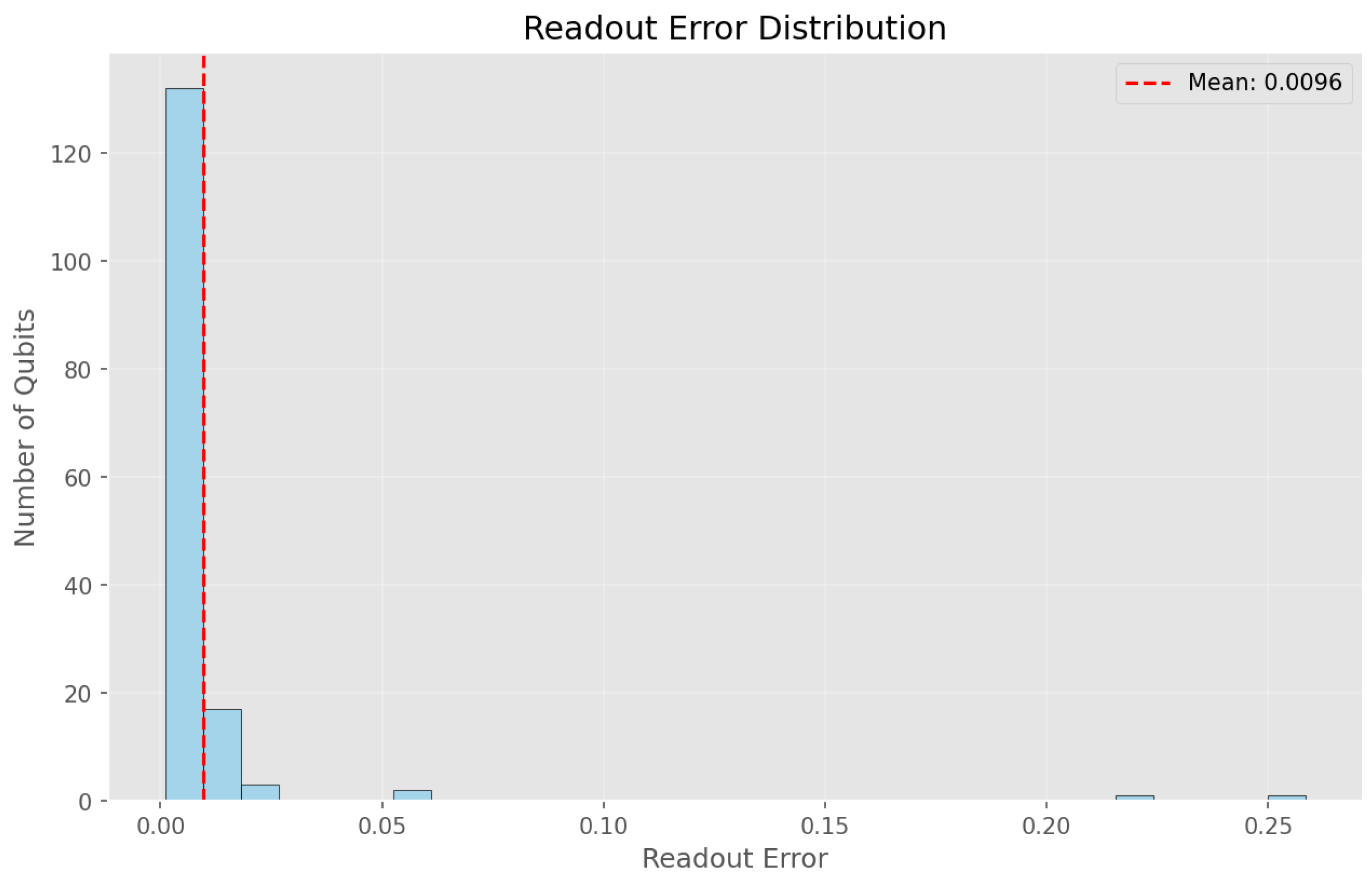
Figure 3.
Spatial categories: and values across four spatial regions.
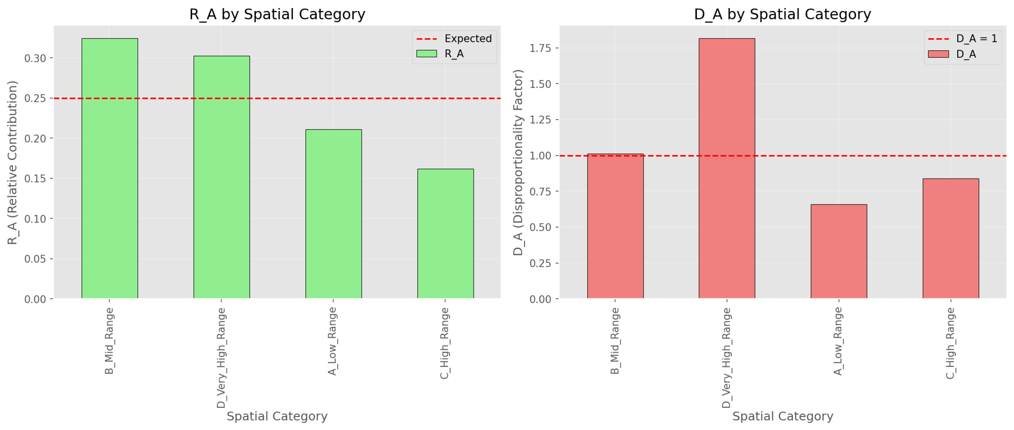
Figure 4.
Error-based categories: and by error rate bins.
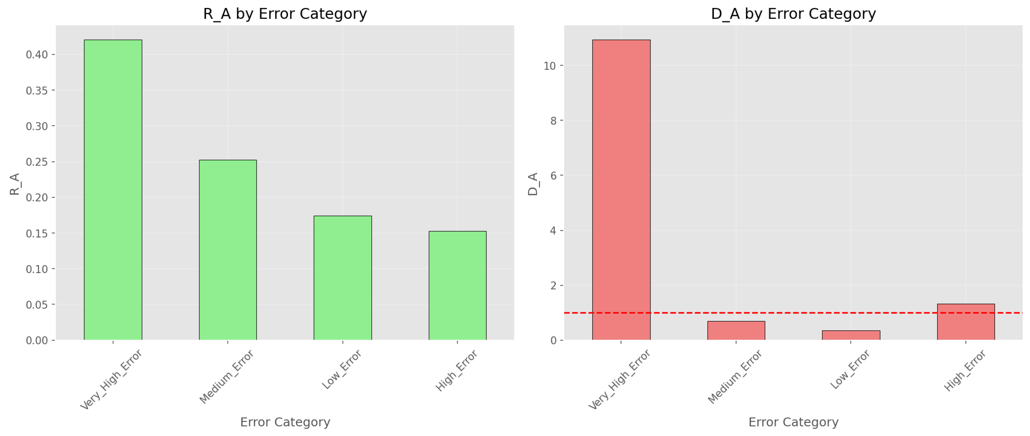
Figure 5.
Coherence-based categories: and by coherence time bins.
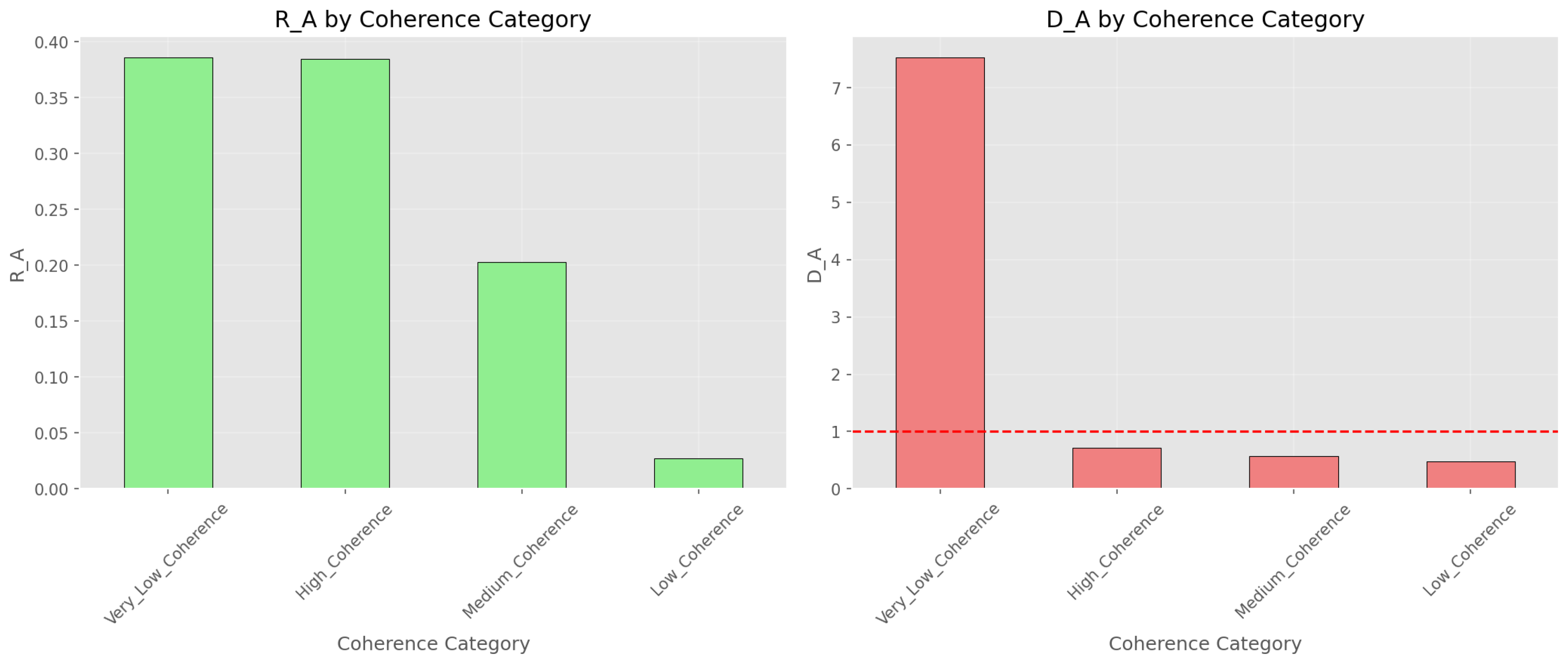
Figure 6.
Category-based metrics comparison. Each subfigure shows the relative contribution (blue bars) and disproportionality factor (orange markers) for different classification schemes. The Very_High_Error and Very_Low_Coherence categories exhibit dramatically elevated values, confirming their disproportionate impact on the total error budget.
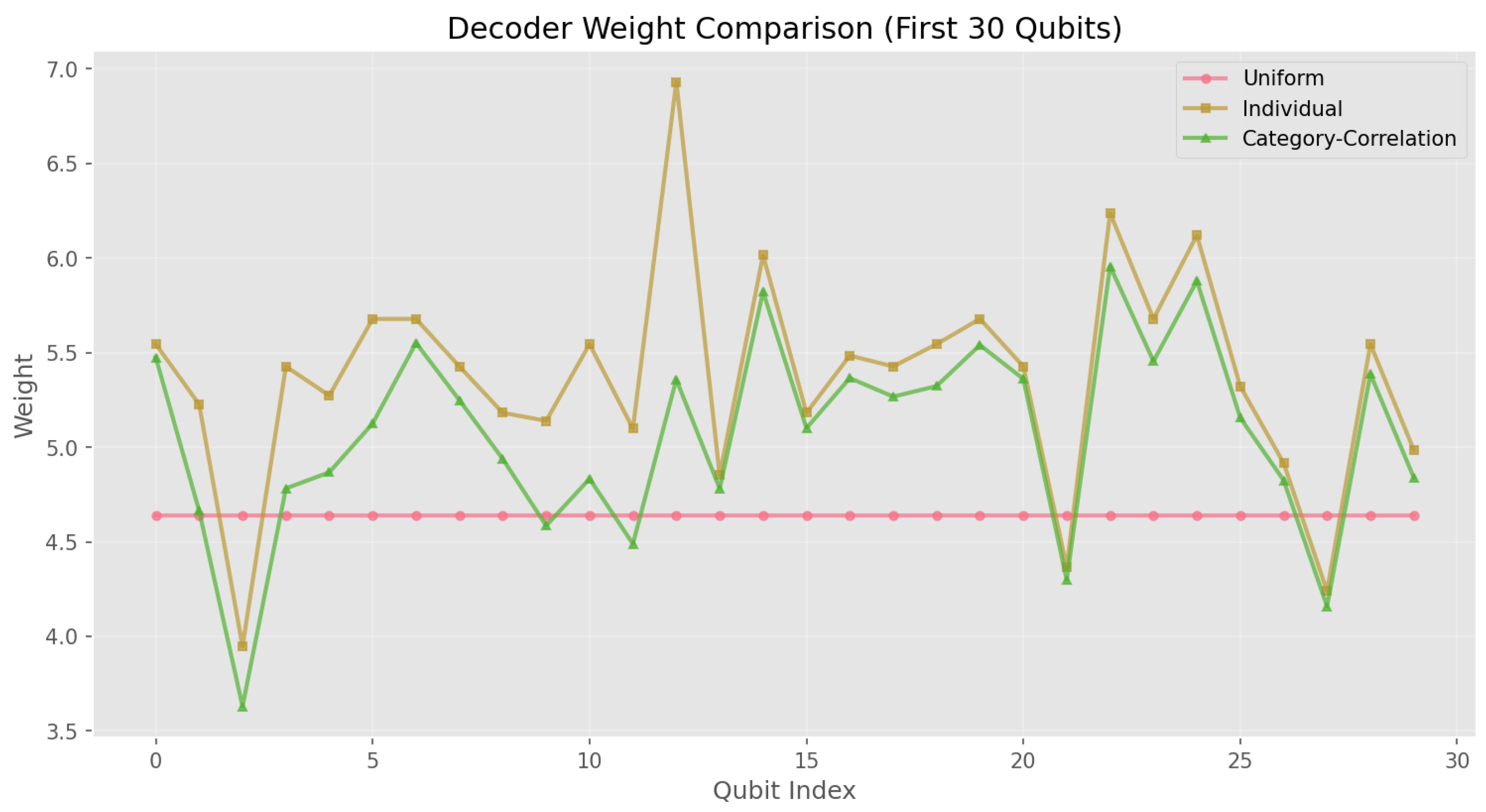
Figure 7.
Decoder weight comparison for the first 30 qubits. Three weighting schemes are shown: uniform (pink), individual per-qubit (orange), and category-correlation aware (green). The category-correlation model assigns significantly higher weights to problematic qubits (e.g., qubits 10-15, 20-25), reflecting their elevated error rates and correlation structure.
8.5. Correlation-Aware Extension
A covariance matrix was constructed using two-qubit gate errors.
- Correlation-induced increase: 129%
High-error correlated pairs indicate the presence of structurally weak nodes in the coupling graph, with qubit 85 appearing repeatedly in high-error connections. Figure 8 visualizes the correlation structure, revealing clusters of strongly correlated qubits that contribute to the 129% increase in the correlation-aware total error estimate.
8.6. Step 7.3 – Decoder Integration
Three decoding weight models were evaluated:
- Uniform weighting
- Individual weighting
- Category-Correlation weighting
Logical Error Rate Estimates
| Model | Description | |
| Uniform | 0.9312 | Global average error |
| Individual | 0.9312 | Per-qubit errors |
| Category-Correlation | 1.7927 | Category and correlation aware |
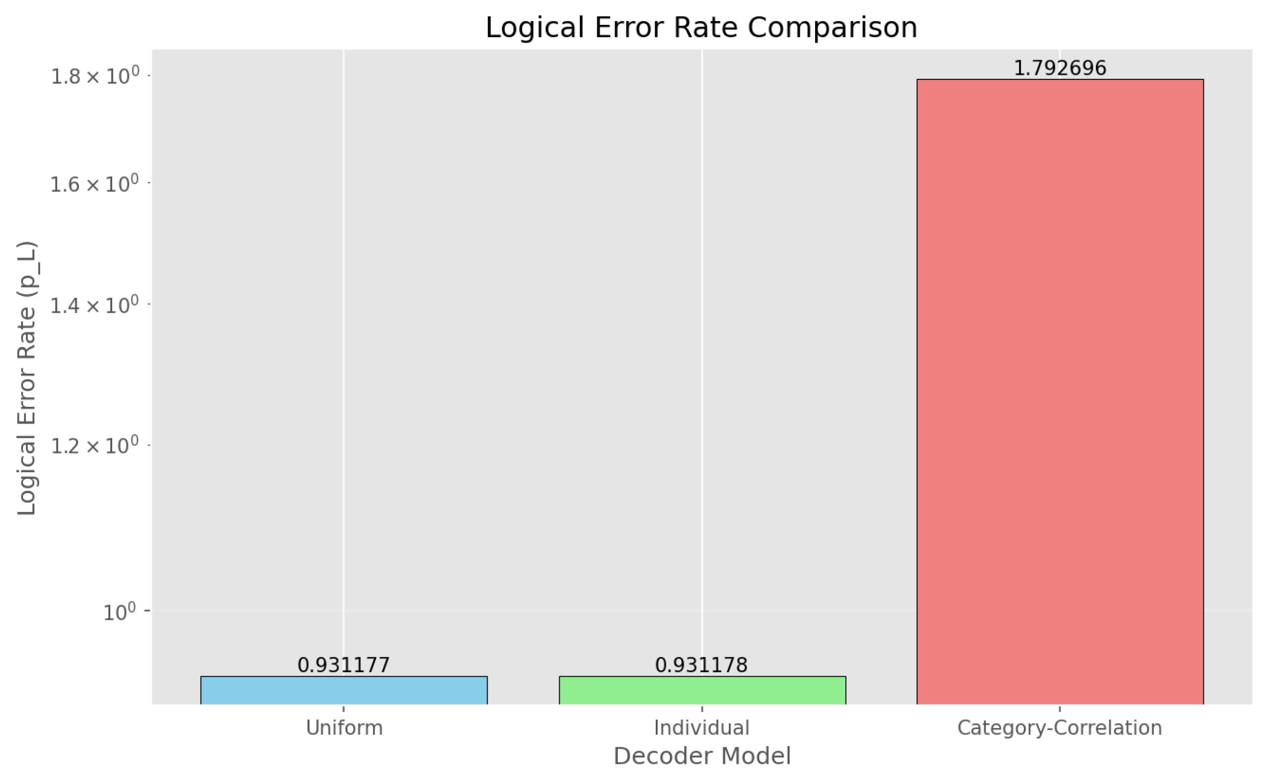
The Category-Correlation model yields a higher logical error estimate. This does not imply worse performance; rather, it reflects a more conservative and realistic estimation under strong heterogeneity and correlated noise. Figure 9 provides a visual comparison of these estimates, while Figure 7 shows how the category-correlation model assigns differentiated weights to individual qubits.
8.7. Identification of Critical Qubits
Problematic qubits include 85, 146, 46, 145, 32, and 113.
Qubit 85:
- Readout error: 0.2178
- Appears in multiple high-error couplings (see Figure 8)
Qubit 146:
- Readout error: 0.2585 (highest in system, see Figure 2 tail)
8.8. Conclusions and Recommendations
- Strong heterogeneity exists: 4% of qubits contribute 42% of total error (Figure 4).
- Ignoring correlations underestimates total error by 129% (Figure 8).
-
Critical categories (Figure 6):
- Very_High_Error ()
- Very_Low_Coherence ()
- D_Very_High_Range (spatial, )
- Further investigation of strong correlated pairs (e.g., 84–85, 85–86, 146–147) is necessary.
- Longitudinal monitoring of the Very_Low_Coherence group is advised.
- Consider circuit remapping to avoid high-error qubits in critical logical paths.
8.9. Final Remarks
The 19 February 2026 calibration analysis demonstrates that while the majority of qubits operate within acceptable error margins, a small subset exerts disproportionate influence on global performance. Figure 2 through Figure 9 collectively illustrate this heterogeneity and its implications for decoder design and error estimation.
The Category-Based Error Budgeting framework successfully identifies these qubits, quantifies their disproportion factors, and integrates correlation structure into logical error estimation. These insights provide a concrete foundation for targeted hardware recalibration and improved decoder design.
Report Date: 22 February 2026
Prepared by: Automated Qubit Performance Analysis System
Source Data:ibm_boston_calibrations_2026-02-19T08_37_34Z
Data Availability Statement
Calibration data and analysis code are available at: https://github.com/jslamja/qubit_analysis_GUI
Acknowledgments
We thank IBM Quantum for providing access to quantum processors and calibration data.
References
- Bravyi, S.; et al. Mitigating measurement errors in multi-qubit experiments. Phys. Rev. A 2021, 103, 042605. [Google Scholar] [CrossRef]
- Endo, S.; Cai, Z.; Benjamin, S. C.; Yuan, X. Hybrid quantum-classical algorithms and quantum error mitigation. J. Phys. Soc. Jpn. 2021, 90, 032001. [Google Scholar] [CrossRef]
- Fowler, A. G.; Mariantoni, M.; Martinis, J. M.; Cleland, A. N. Surface codes: Towards practical large-scale quantum computation. Phys. Rev. A 2012, 86, 032324. [Google Scholar] [CrossRef]
- Dennis, E.; Kitaev, A.; Landahl, A.; Preskill, J. Topological quantum memory. J. Math. Phys. 2002, 43, 4452–4505. [Google Scholar] [CrossRef]
- Temme, K.; Bravyi, S.; Gambetta, J. M. Error mitigation for short-depth quantum circuits. Phys. Rev. Lett. 2017, 119, 180509. [Google Scholar] [CrossRef]
- Gambetta, J. M.; et al. Characterization of addressability by simultaneous randomized benchmarking. Phys. Rev. Lett. 2012, 109, 240504. [Google Scholar] [CrossRef] [PubMed]
- Chubb, C. T.; Flammia, S. T. Statistical mechanical models for quantum codes with correlated noise. Ann. Inst. Henri Poincaré D 2021, 8, 269–321. [Google Scholar] [CrossRef]
- Quantum AI, Quantum AI. Exponential suppression of bit or phase flip errors with repetitive error correction. Nature 2021, 595, 383–387. [Google Scholar] [CrossRef] [PubMed]
- Arute, F.; et al. Quantum supremacy using a programmable superconducting processor. Nature 2019, 574, 505–510. [Google Scholar] [CrossRef] [PubMed]
- Kelly, J.; et al. State preservation by repetitive error detection in a superconducting quantum circuit. Nature 2015, 519, 66–69. [Google Scholar] [CrossRef] [PubMed]
- Delfosse, N.; Nickerson, N. H. Almost-linear time decoding algorithm for topological codes. Quantum 2021, 5, 595. [Google Scholar] [CrossRef]
- Proctor, T.; Rudinger, K.; Young, K.; Nielsen, E.; Blume-Kohout, R. Measuring the capabilities of quantum computers. Phys. Rev. Lett. 2022, 128, 230502. [Google Scholar] [CrossRef]
- Chuang, I. L.; Gershenfeld, N.; Kubinec, M. Experimental implementation of fast quantum searching. Phys. Rev. Lett. 1998, 80, 3408–3411. [Google Scholar] [CrossRef]
- Vandersypen, L. M. K.; et al. Experimental realization of Shor’s quantum factoring algorithm using nuclear magnetic resonance. Nature 2001, 414, 883–887. [Google Scholar] [CrossRef]
- Clarke, J.; Wilhelm, F. K. Superconducting quantum bits. Nature 2008, 453, 1031–1042. [Google Scholar] [CrossRef]
- DiCarlo, L.; et al. Demonstration of two-qubit algorithms with a superconducting quantum processor. Nature 2009, 460, 240–244. [Google Scholar] [CrossRef]
- Kandala, A.; et al. Hardware-efficient variational quantum eigensolver. Nature 2017, 549, 242–246. [Google Scholar] [CrossRef]
- Murali, P.; et al. Noise-adaptive compiler mappings for NISQ computers. ASPLOS 2019, 1015–1029. [Google Scholar] [CrossRef]
- Linke, N. M.; et al. Experimental comparison of two quantum computing architectures. Proc. Natl. Acad. Sci. USA 2017, 114, 3305–3310. [Google Scholar] [CrossRef] [PubMed]
- Klimov, P. V.; et al. Fluctuations of energy-relaxation times in superconducting qubits. Phys. Rev. Lett. 2018, 121, 090502. [Google Scholar] [CrossRef] [PubMed]
- Havlíček, V.; et al. Supervised learning with quantum-enhanced feature spaces. Nature 2019, 567, 209–212. [Google Scholar] [CrossRef] [PubMed]
- Cross, A. W.; et al. Validating quantum computers using randomized model circuits. Phys. Rev. A 2019, 100, 032328. [Google Scholar] [CrossRef]
- Wack, A.; et al. Quality, Speed, and Scale: Measuring performance of near-term quantum computers. arXiv 2021, arXiv:2110.14108. [Google Scholar]
- Cerezo, M.; et al. Variational quantum algorithms. Nat. Rev. Phys. 2021, 3, 625–644. [Google Scholar] [CrossRef]
Figure 8.
Correlation matrix visualization for qubit pairs with significant covariance. The color scale ranges from blue (negative correlation) through white (zero) to red (positive correlation). High-error qubits (e.g., qubit 85) appear repeatedly in strongly correlated pairs, indicating structurally weak nodes in the coupling graph.
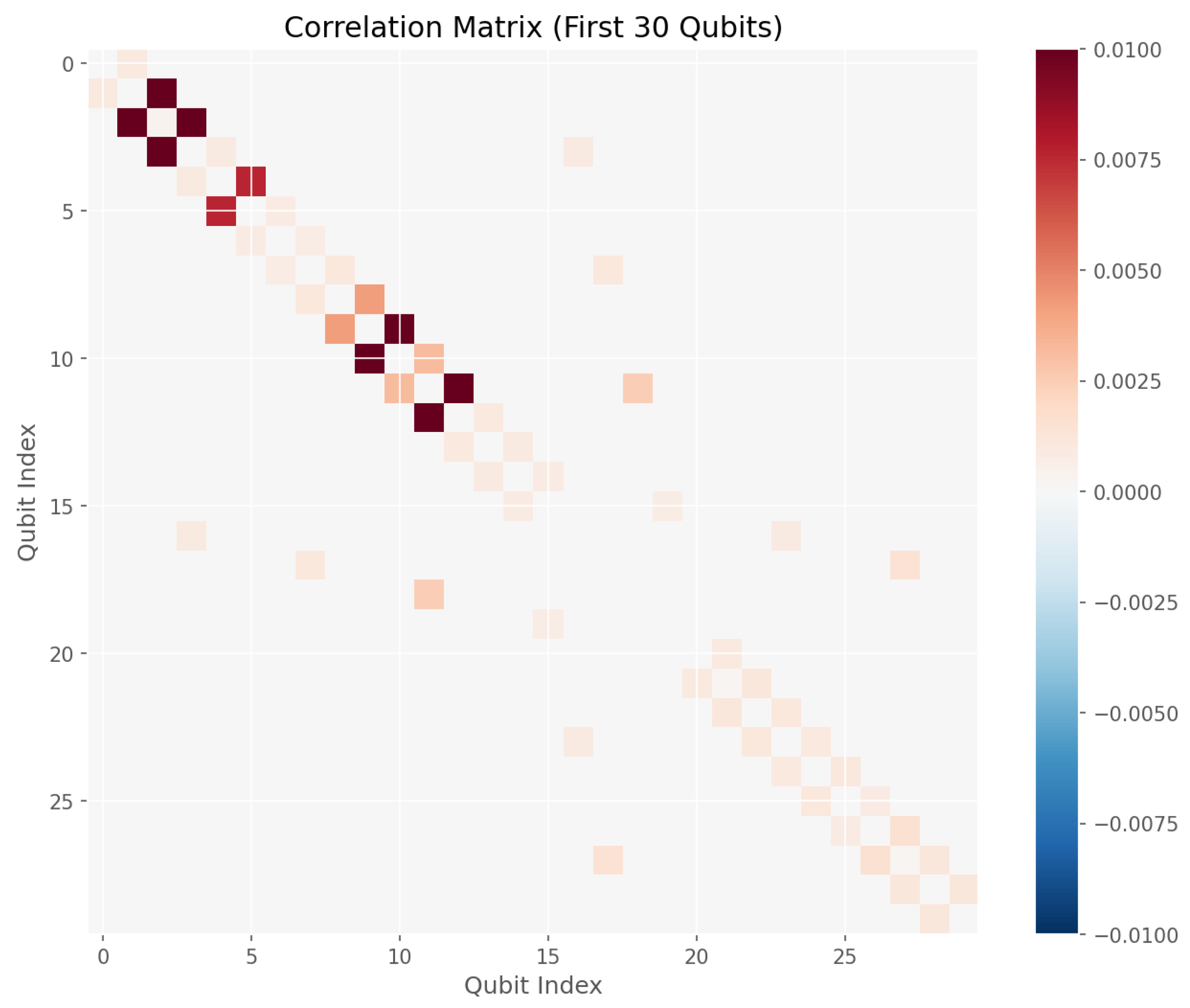
Figure 9.
Logical error rate estimates for three decoder weighting models. The uniform and individual models yield nearly identical values (), while the category-correlation model produces a substantially higher estimate (). This reflects a more conservative and realistic assessment under strong heterogeneity and correlated noise.
Disclaimer/Publisher’s Note: The statements, opinions and data contained in all publications are solely those of the individual author(s) and contributor(s) and not of MDPI and/or the editor(s). MDPI and/or the editor(s) disclaim responsibility for any injury to people or property resulting from any ideas, methods, instructions or products referred to in the content. |
© 2026 by the authors. Licensee MDPI, Basel, Switzerland. This article is an open access article distributed under the terms and conditions of the Creative Commons Attribution (CC BY) license (http://creativecommons.org/licenses/by/4.0/).
Copyright: This open access article is published under a Creative Commons CC BY 4.0 license, which permit the free download, distribution, and reuse, provided that the author and preprint are cited in any reuse.


