Submitted:
25 February 2026
Posted:
27 February 2026
You are already at the latest version
Abstract
The coupled logistic models developed in this study, across various media (concen-trated whey (CW), diluted whey (DW), MRS, and TGE broths) and nutrient (glutamic acid or glucose) supplementation levels, revealed clear patterns in model performance for six culture variables. Biomass growth, lactic acid (LA) production, total antibacte-rial activity (TAA) synthesis, and pH evolution were generally well described by both uncoupled and coupled logistic models, with R² values above 0.9700. Coupling pro-vided moderate improvements for LA and TAA, particularly in glucose-supplemented DW media, by linking metabolite formation to biomass growth and pH decline, result-ing in more mechanistically and physiologically coherent models. The most pro-nounced benefits of coupling were observed for the consumption of total sugars (TS) and nitrogen (TN). In uncoupled models, R² values for TS and TN were often low or highly variable, whereas coupled models substantially increased R² (up to ~0.9990). These findings demonstrate that TS and TN consumption are strongly growth-associated processes and cannot be adequately modeled as independent phe-nomena. Overall, while uncoupled models are sufficient to describe growth, acidifica-tion, and metabolite formation, the coupled modeling approach provides a robust, in-tegrated framework that captures the interactions among biomass growth, nutrient utilization, and metabolite production.
Keywords:
batch fermentation kinetics
; uncoupled logistic modeling
; coupled logistic modeling
; lactic acid bacteria
1. Introduction
Lactic acid bacteria (LAB) are widely used in food fermentations and biotechnological applications, where the efficiency of biomass production and substrate utilization directly affects product yield and process optimization [1,2,3].
These bacteria produce organic acids (mainly lactic acid) through the catabolism of sugars present in the substrate, leading to a decrease in culture pH [3,4]. Biomass accumulation critically depends on culture pH, as it influences cellular metabolism, intracellular homeostasis, enzyme activity, and nutrient uptake [4,5,6,7]. Previous studies have shown that biomass production reaches a maximum within an optimal pH range (e.g., near neutral or mildly acidic conditions) for many LAB strains. In contrast, excessively low pH values significantly reduce biomass accumulation and may even lead to cell death, as acid stress inhibits metabolism and cell division [8,9,10] and can impair LAB growth more severely than nutrient depletion [4,11].
Acid accumulation increases the proportion of undissociated acid species, which can diffuse back into the cell, dissipate the proton motive force, and drain cellular energy as bacteria expel excess protons—ultimately inhibiting growth and reducing biomass yield [12,13,14,15]. Thus, in LAB fermentations, biomass formation is directly linked to the availability of growth-limiting nutrients, particularly nitrogen sources, and is strongly modulated by culture acidification resulting from lactic acid production [4,16,17].
LAB are also capable of producing bacteriocins—antibacterial peptides often considered pH-dependent primary metabolites—which are highly sensitive to the time course of culture pH during fermentation [18]. Therefore, changes in culture pH can modulate bacteriocin synthesis [19,20], likely through regulation of biosynthetic genes [21,22], modulation of the enzymatic activity responsible for post-translational processing of prebacteriocins into their active forms [15,23], and adsorption of bacteriocins to the cell wall of the producer strain [24].
Furthermore, total sugar and nitrogen consumption are governed by biomass production, as these nutrients serve as energy sources to support growth and cellular maintenance, are incorporated into new biomass, and are utilized for metabolite production [17,25,26].
Mathematical modeling of LAB fermentations is an essential tool for understanding, predicting, and optimizing microbial growth, metabolite production, and substrate utilization in complex culture systems [25]. Among the available empirical approaches, logistic-type equations have been widely and successfully applied to describe batch biomass growth, lactic acid formation, antimicrobial metabolite production, substrate consumption, and pH evolution during LAB fermentations due to their simplicity and good fitting performance across different media and strains [27,28,29,30]. These models assume self-limiting behavior and capture the sigmoidal dynamics typically observed in batch cultures [27,28].
However, a major limitation of these equations is that they describe culture variables solely as functions of time, implicitly assuming that microbial growth, product formation, and nutrient consumption in batch cultures are purely autocatalytic processes. Moreover, such models do not explicitly account for the underlying biological and biochemical mechanisms driving growth, metabolite production, and nutrient utilization in LAB fermentations.
Consequently, treating kinetic parameters—such as growth, production, and consumption rates—as independent constants may limit the predictive power and physiological relevance of these models.
By linking the kinetic parameters of the logistic equations through biologically meaningful relationships—accounting for pH effects, nutrient limitation, and growth–production coupling—the proposed approach provides a more precise, comprehensive, and integrated description of LAB fermentation dynamics while retaining the mathematical simplicity of logistic models. Such models not only enhance our understanding of microbial physiology but also provide practical benefits for the design and control of fermentation processes. This approach may improve the predictive accuracy of growth models and support the optimization of culture conditions, ultimately contributing to more efficient fermentation processes and a deeper understanding of microbial physiology.
To address the limitations of logistic-type equations in describing the kinetics of LAB fermentation, the present study focuses on developing an improved modeling framework based on coupled logistic models that incorporate the relationships among biomass growth, lactic acid production, total antibacterial activity, pH evolution, and nutrient consumption (total sugars and nitrogen).
2. Materials and Methods
2.1. Bacterial Strains
The bacterial strains used in this study were Lactococcus lactis subsp. lactis CECT 539, Lactobacillus casei subsp. casei CECT 4043 (both obtained from the Spanish Type Culture Collection, CECT), and Pedicoccus acidilactici NRRL B-5627 (obtained from the Northern Regional Research Laboratory, NRRL, Peoria, IL, USA). These strains were used as producer of lactic acid (LA) and total antibacterial activity (TAA) in the different culture media.
The three bacterial strains were initially grown at 30 ºC in MRS (de Man, Rogosa, and Sharpe) broth for 24 h, and an aliquot (1 mL) was used to inoculate 50 mL of the corresponding fermentation medium (Table 1). These pre-cultures were incubated at 30 ºC and 200 rpm in an orbital shaker for 12 h. Subsequently, the main fermentations were carried out by inoculating 1 mL of the respective pre-culture into the corresponding fermentation medium (Table 1).
2.2. Culture Media, Fermentation Conditions and Data Collection
The culture media used in the batch cultures of L. lactis CECT 539, Lact. casei CECT 4043, and Ped. acidilactici NRRL B-5627 are summarized in Table 1. During these fermentations, the concentrations of biomass (X(t), in g/L), lactic acid (LA(t), in g/L), and total antibacterial activity (TAA(t), in activity units (AU)/mL), along with culture pH, total sugars (TS(t), in g/L) and nitrogen (TN(t), in g/L), were measured at regular intervals [31,32,33,34,35,36].
The values of these culture variables were used to develop coupled logistic equations from the corresponding uncoupled logistic equations, providing a more accurate description of the time courses of all six variables in the different batch cultures.
The applicability of the coupled logistic equations was further tested using data on culture pH, biomass, and bacteriocin (a component of TAA) produced by Pediococcus acidilactici LB42–923, Lactococcus lactis subsp. lactis ATCC 11454, Leuconostoc carnosum Lm1, and Lactobacillus sakei LB 706 in 18–h batch cultures in TGE medium [23]. Each culture was incubated at its respective optimum temperature. The culture pH, biomass, and bacteriocin data were extracted from the publication by Yang and Ray [23] using GetData Graph Digitizer 2.24 software.
2.3. Analytical Determinations
The concentrations of biomass, X(t); lactic acid, LA(t); total antibacterial activity, AA(t); total sugars, TS(t); and total nitrogen, TN(t), in batch cultures of Lactococcus lactis subsp. lactis CECT 539, Lactobacillus casei CECT 4043, and Pediococcus acidilactici NRRL B-5627 were determined using the methods described in previous studies [31,32,33,34,35,36]. The initial concentrations of TS and TN in TGE medium were measured according to the procedures reported in the same references [31,32,33,34,35,36].
Analytical determinations of biomass and bacteriocins produced by Pediococcus acidilactici LB42–923, Lactococcus lactis subsp. lactis ATCC 11454, Leuconostoc carnosum Lm1, and Lactobacillus sakei LB 706 have been previously described by Yang and Ray [23].
2.4. Models Improvement
2.4.1. Uncoupled Models
Batch biomass growth, X(t), as well as the productions of lactic acid, LA(t), and antibacterial activity, TAA(t), by lactic acid bacteria (LAB) in various culture media have commonly been described using the simplest form of the logistic equation [27,28,29,37], as shown below:
Where KX, KLA, and KTAA represent the maximum biomass concentration (g/L), lactic acid concentration (g/L), and total antibacterial activity (AU/mL), respectively. The constants aX, aLA, and aTAA are dimensionless, whereas bX, bLA, and bTAA denote the rates (h−1) of biomass growth, lactic acid production, and total antibacterial activity synthesis, respectively. The variable t denotes the fermentation time (h).
The decrease in culture pH, pH(t), has usually been described using the von Bertalanffy equation (4) [27].
Where pHi and pHf represent the initial and final culture pH values, respectively; and bpH denotes the rate constant (h−1) of pH decrease.
In this case, at t = 0 h, pH0 = pHi, and as t → ∞, pH∞ = pHf.
Because the pH evolution in LAB cultures generally follows a decreasing pattern [23,27,37], similar to that observed for nutrients (total sugars, nitrogen, proteins, and phosphorus) [27,28,37], equation (5), originally proposed for nutrient consumption [28], can also be used to describe pH evolution in LAB cultures:
In this case, at t = 0 h:
and as t → ∞, pH∞ = pHf.
In the case of DW medium, equations (4) and (5) adequately fitted the experimental pH data (Figure 1), which exhibited a C-shaped profile. However, these equations did not always provide an optimal description of pH decrease, particularly when the pH followed a typical inverted S-shaped profile, as observed in MRS and TGE broths (Figure 1).
The differences between the pH profiles in DW medium and those in MRS and TGE broths may be attributed to variations in the buffering capacity of these culture media [38], which reflects their resistance to changes in the initial culture pH due to the presence of proteins, amino acids, and salts with buffering properties [39]. Commercial broths contain higher protein concentrations (13.32 ± 0.021 g/L in MRS broth [32] and 10.22 ± 0.61 g/L in TGE broth) than deproteinized diluted whey (2.04 ± 0.08 g/L) [33]. Consequently, the buffering capacity of the commercial media (MRS and TGE) is higher.
Therefore, in this study, model (4) was modified by introducing a constant (BC) in the numerator to account for the buffering capacity of the culture medium on the pH time course. In addition, the denominator of the model was modified to smooth the rate of pH decrease, as follows:
Where apH is a dimensionless constant.
With this approach, model (6) describes pH changes in LAB fermentations as a function of organic acid production (mainly lactic acid) and the buffering capacity of the culture medium [40].
At t = 0 h:
Considering that at t = 0 h, pH0 = pHi, then:
Substituting BC into model (6) gives:
Similarly, as t → ∞, pH∞ = pHf.
As shown in Figure 1, model (6) provided the best fit to the experimental pH data, accurately describing both C-shaped and inverted S-shaped profiles in the three culture media, with higher R² values. Therefore, this model was used to describe the pH profiles in the different culture media (CW; unsupplemented DW; DW supplemented with glutamic acid or glucose; unsupplemented and glutamic acid-supplemented MPW; and MRS and TGE broths).
To describe the time courses of total sugars, TS(t), and total nitrogen, TN(t), the following models were used:
Where TSi and TSf, and TNi, TNf, represent the initial and final concentrations (g/L) of total sugars (TS) and total nitrogen (TN), respectively. The constants aTS and aTN are dimensionless, whereas the parameters bTS and bTN represent the rate constants (h−1) for TS and TN consumption, respectively.
2.4.2. Development of Coupled Models
Since biomass growth, the synthesis of both lactic acid and antibacterial activity, culture pH evolution, and the consumption of total sugars and nitrogen are measured simultaneously during fermentation, time-independent relationships among all six variables can be derived by eliminating the fermentation time variable. To achieve this, t is isolated from models (1), (2), (3), (6), (7), and (8).
Starting from model (1):
Taking the natural logarithm yields:
Therefore:
Applying the same procedure to models (2) and (3) gives:
For models (6) to (8):
Since LAB growth depends on the evolution of culture pH [21,27,31,32,40], the parameter bX in model (9) can be corrected to account for this effect. For this purpose, the relationships between bX and bpH was derived by equating model (9) with model (12).
Solving for bX gives:
Where bpH–X represents the rate of biomass formation as affected by pH.
Substituting bX into model (1) gives:
Proceeding in the same way for lactic acid and antibacterial activity, and considering that lactic acid is produced by LAB cells and that antibacterial activity is a primary metabolite whose production depends on the pH time course [23,27,31,37,41], the synthesis of both compounds can be expressed as:
Where bX–LA represents the rate of lactic acid production as affected by biomass growth, and bX–TAA and bpH–TAA represent the rates of total antibacterial activity synthesis as affected by biomass growth and pH, respectively.
Since the reduction in culture pH is caused by lactic acid production by growing LAB cells, the relationship between bpH and bX can be obtained by equating models (9) and (12). Therefore, the culture pH evolution could be expressed as:
Where bLA–pH represents the rate of pH decline as influenced by lactic acid production.
Considering that total sugars and nitrogen are consumed by the growing LAB cells, the coupled logistic models for nutrient consumption can be expressed as:
Where bX–TS and bX–TN represent the rates of total sugars and total nitrogen consumption, respectively, as influenced by biomass growth.
Although more complex relationships among the six culture variables could be derived, the simple coupled models (16)–(21) provide a tighter relationship among the variables, indicating that the change in one variable is driven by the effect of another.
2.5. Model Parameters Determination and Model Evaluation
Experimental data on the kinetics of biomass growth, lactic acid production, total antibacterial activity synthesis, culture pH, and the consumption of total sugars and nitrogen from triplicate fermentations in different culture media [31,32,33,34,35,36] were used to develop the coupled models and estimate the corresponding model parameters. The values of the constants were initially obtained by minimizing the sum of squared differences between the experimental and model-predicted values using the nonlinear least-squares (quasi-Newton) method implemented via the Solver tool in Microsoft Excel 2016 (Microsoft Corp., Redmond, WA, USA). To avoid overestimation of the initial values of each culture variable (X, LA, TAA, pH, TS, and TN) during the fitting of the models to the experimental data, a constraint was applied in all cases requiring that the model-predicted values at time zero (Yp0) match the corresponding experimental values (Yexp0).
The corresponding R2 values for the models were determined using the same Microsoft Excel spreadsheet.
The uncoupled models were independently fitted to the corresponding experimental data by minimizing the sum of squared differences (SSD) between the experimental values (Yexpᵢ) of biomass (X), lactic acid (LA), total antibacterial activity (TAA), culture pH, total sugars (TS), and nitrogen (TN), and the corresponding predicted values (Ypᵢ) generated by the models:
In the case of coupled models, which share some parameters (models (16)–(21)), the model constants were simultaneously estimated by minimizing the total sum of squared differences (SSDT) between the experimental values (expᵢ) of the six culture variables (X, LA, TAA, pH, TS, and TN) and their corresponding predicted values (pᵢ) generated by the models:
Lower SSD values and higher R2 values indicate a better fit and greater accuracy of the models in describing the trends observed in the experimental data.
3. Results and Discussion
The efficacy of the coupled logistic models (16)–(21) in describing the time courses of six culture variables—namely biomass growth (X), product formation (LA and TAA), culture pH, and nutrient consumption (TS and TN)—was demonstrated using experimental data from three lactic acid bacteria strains (CECT 539, CECT 4043, and NRRL B–5627) cultivated in different culture media [31,32,33,34,35,36].
To further validate the accuracy of the proposed models in describing the six culture variables, the results obtained from the coupled models (16)–(21) were compared with those generated by the corresponding unmodified logistic models (1), (2), (3), (6), (7), and (8).
In addition, the models were validated using data from batch cultures of Pediococcus acidilactici LB42–923 (a pediocin AcH producer), Lactococcus lactis subsp. lactis ATCC 11454 (a nisin producer), Leuconostoc carnosum Lm1 (a leuconocin Lcm1 producer), and Lactobacillus sakei LB 706 (a sakacin A producer), grown in TGE broth at uncontrolled pH [23].
As only experimental data on growth, bacteriocin production, and pH time courses were available in this case [23], only models (16), (18), and (19) were validated, and the corresponding results were compared with those obtained using the unmodified models (1), (3), and (6), respectively.
Considering that lactic acid is primarily a growth-associated product, as it is predominantly synthesized by LAB strains during the active growth phase [30,42], model (19) was modified by substituting the lactic acid time-course data, LA(t), and its corresponding constants (KLA and aLA) with those of biomass growth (X(t), KX, and aX), as indicated below:
Where bX–pH represents the rate of pH decline as influenced by biomass growth.
3.1. Modeling Batch Growth, Product Formation, and Nutrient Consumption by Lactococcus lactis CECT 539 in Concentrated Whey and MRS Broth
3.1.1. Uncoupled Models
Figure 2A shows the time courses of experimental biomass growth, lactic acid production, total antibacterial activity synthesis, culture pH, and consumption of total sugars and nitrogen by strain CECT 539 in concentrated whey (CW) and MRS broth, together with the predictions of models (1), (2), (3), (6), (7), and (8).
For the CW culture (Figure 2A and Table 2), models (1), (3), and (6) provided an adequate description of the experimental data for biomass growth (R2X = 0.9846, SSD–X = 2.29 × 10⁻³), total antibacterial activity production (R²TAA = 0.9838, SSD–TAA = 1.18), and culture pH (R²pH = 0.9952, SSD–pH = 6.12 × 10⁻³). However, models (2), (7), and (8) did not satisfactorily describe the time courses of lactic acid (R²LA = 0.9500, SSD–LA = 2.58 × 10⁻²), total sugars (R²TS = 0.9638, SSD–TS = 3.34), and total nitrogen (R²TN = 0.9512, SSD–TN = 8.27 × 10⁻³), respectively (Figure 2A and Table 2).
The failure of model (2) to adequately describe the kinetics of lactic acid synthesis in CW medium can be attributed to the fact that lactic acid production did not follow the typical logistic-type profile observed in MRS broth (see the upper right panel of Figure 2A). Even when the constraint requiring that the model-predicted values at time zero (Yp₀) match the corresponding experimental values (Yexp₀) was removed, the R²LA value increased to 0.9793 and the SSD–LA decreased to 1.18 × 10⁻². However, the predicted initial lactic acid concentration increased to 0.082 g/L, which is considerably higher than the experimental value (0.016 g/L).
The relatively low R2 obtained for models (7) and (8) can be explained by the fact that the time courses of total sugars (TS) and total nitrogen (TN) did not strictly follow a C-shaped profile during CW fermentation (see the lower left and lower right panels of Figure 2A).
With regard to the culture in MRS broth, the modeling results were slightly better than those obtained in CW medium (Figure 2A), with higher R2 values (0.9979, 0.9981 and 0.9809) obtained for models (1), (2), and (7), respectively (Table 2). However, the predictions of models (3), (6), and (8) for the kinetics of total antibacterial activity (TAA) synthesis, culture pH, and total nitrogen (TN) were similar in both culture media, yielding comparable R2 values.
The differences observed in the predictions of the models (1), (2), (3), (6), (7), and (8) between fermentations conducted in the two culture media can be attributed solely to the degree of agreement between the experimental time-course data for the corresponding culture variables and the mathematical structure of each model.
3.1.2. Coupled Models
Uncoupled models assume that each variable evolves independently with its own logistic time constant. In LAB fermentations, the growth, the synthesis of lactic acid and total antibacterial activity, pH drop and consumption of nutrients (TS and TN) are not independent processes evolving only with time, because, fermentation is a closed biochemical network, not six independent time–driven phenomena [27,29,30,31,32]. Then, developing of coupled models could reflect this biological interdependence.
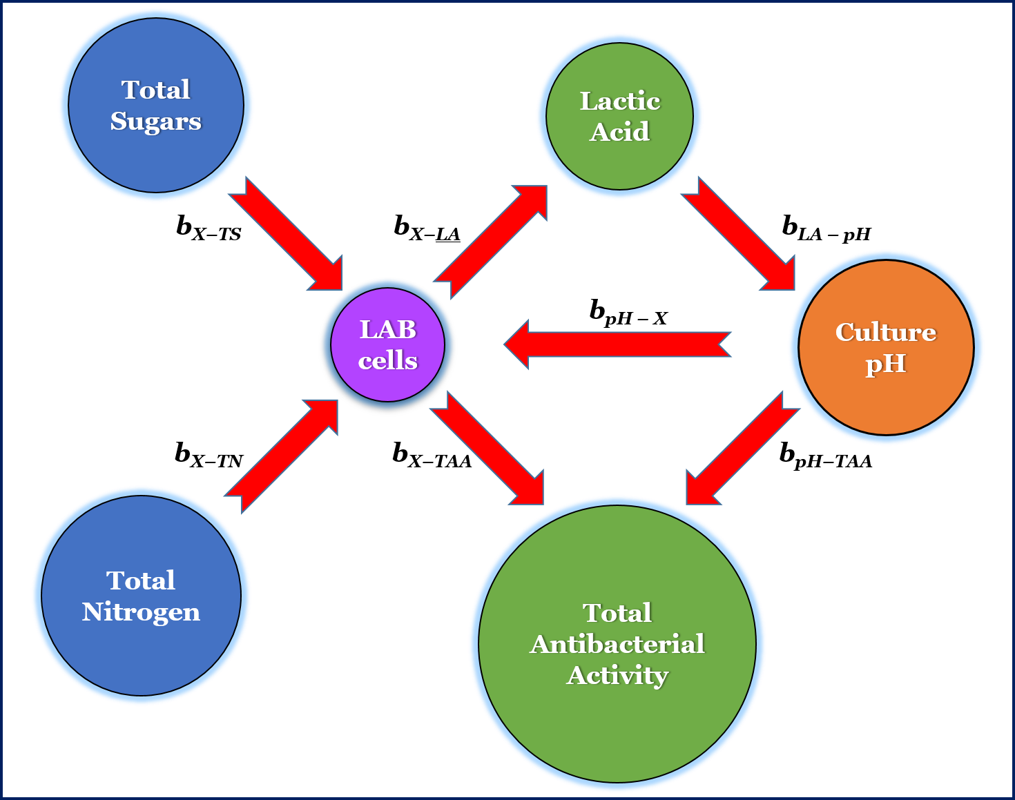
In this study, the following simple biologically linked through cause–effect relationships between the six variables were assumed: i) pH affects cell growth kinetics, ii) lactic acid production decreases pH, iii) primary metabolite production (LA) depends on growth, iv) antibacterial activity depends on both biomass and pH evolution and, v) biomass formation drives sugar and nitrogen consumption.
The coupled models (16)–(21) were fitted simultaneously to the experimental data for the six culture variables (X, LA, TAA, pH, TS, and TN), incorporating biologically meaningful cause–effect relationships among them. The statistical performance of these models in concentrated whey (CW) and MRS broth is summarized in Table 3, and the corresponding fits are presented in Figure 2B.
In CW medium, the coupled formulation significantly improved the overall description of the fermentation process compared with the uncoupled approach (Table 2 and Table 3). The coupled biomass model provided an excellent fit (R²X = 0.9962; SSD–X = 6.25 × 10⁻⁴), outperforming the uncoupled model (R²X = 0.9846; SSD–X = 2.29 × 10⁻³). The approximately one-order-of-magnitude reduction in SSD–X indicates that incorporating the pH-dependent correction of the growth parameter (bpH–X = 0.29 h⁻¹) enhanced the representation of growth dynamics. This confirms that biomass evolution in CW is strongly influenced by culture acidification.
In contrast, the coupled model did not substantially improve the description of lactic acid production (R²LA = 0.9492; SSD–LA = 3.99 × 10⁻²) compared with the uncoupled model (R²LA = 0.9500; SSD–LA = 2.58 × 10⁻²). The lower goodness-of-fit reflects the deviation of lactic acid production in CW from a strictly logistic profile (Figure 2A and 2B). Although coupling with biomass (bX–LA = 0.51 h⁻¹) ensures biological consistency, it does not fully capture the irregular kinetic pattern observed experimentally. This suggests that additional metabolic constraints or substrate limitations may influence acid synthesis in CW.
A marked improvement was observed for TAA production (R²TAA = 0.9943; SSD–TAA = 0.47) compared with the uncoupled model (R²TAA = 0.9838; SSD–TAA = 1.18). The simultaneous dependence on biomass (bX–TAA = 0.23 h⁻¹) and pH (bpH–TAA = 0.12 h⁻¹) enhanced the predictive capacity of the model. The lower SSD indicates that antibacterial activity is better described when both growth and acidification effects are considered, supporting its classification as a growth-associated metabolite influenced by environmental pH.
Although the fit remained acceptable (R²pH = 0.9750), the coupled pH model showed a lower R² and higher SSD–pH (4.13 × 10⁻²) than the uncoupled formulation (R²pH = 0.9952; SSD–pH = 6.12 × 10⁻³). This slight deterioration is likely due to the imposed dependence of pH on lactic acid production (bLA–pH = 0.83 h⁻¹), which did not follow a strictly logistic time profile (Figure 2A and 2B). Nevertheless, the coupled model ensures mechanistic coherence between acid production and pH decline.
A substantial improvement was observed for sugar consumption. The R²TS increased from 0.9638 to 0.9926, while SSD–TS decreased from 3.34 to 0.56. By directly linking total sugar (TS) consumption to biomass formation (bX–TS = 0.40 h⁻¹), the coupled model more accurately represented substrate depletion, confirming that sugar utilization is primarily growth-driven rather than purely time-dependent.
An even more pronounced improvement was observed for nitrogen consumption. The R²TN increased from 0.9512 to 0.9954, and SSD–TN decreased by nearly one order of magnitude (from 8.27 × 10⁻³ to 8.88 × 10⁻⁴). This indicates that total nitrogen (TN) depletion is strongly correlated with biomass production (bX–TN = 0.44 h⁻¹), and that the coupling strategy effectively captures this relationship.
Overall, in CW medium, the coupled models improved the description of biomass, TAA, TS, and TN, maintained a similar fit for lactic acid, and slightly reduced the statistical performance for pH. Nevertheless, the coupled system provides a more coherent and biologically consistent representation of the fermentation process (Table 2 and Table 3).
In MRS broth, where the uncoupled models already provided excellent fits, the improvements introduced by coupling were less pronounced, although still relevant.
For biomass, R²X decreased slightly from 0.9979 to 0.9938, and the SSD–X increased modestly. Nevertheless, the fit remained excellent, and the growth–pH interaction (bpH–X = 0.51 h⁻¹) confirms that acidification influences growth even in a nutritionally rich medium.
For lactic acid (LA) synthesis, the coupled model slightly reduced R²LA (0.9915 vs. 0.9981), although the fit remained very good. Because LA production in MRS follows a well-defined logistic profile, the uncoupled model was already sufficient (Figure 2A); thus, coupling mainly improved mechanistic interpretation rather than statistical performance.
In the case of the TAA model, a slight improvement was observed (R²TAA = 0.9958 vs. 0.9856), accompanied by a marked reduction in SSD–TAA (0.12 vs. 42.07). The dual dependence on biomass and pH significantly enhanced model accuracy, highlighting the synergistic regulation of antibacterial compound synthesis (Figure 2A and 2B).
The coupled pH model slightly improved the fit (R²pH = 0.9969 vs. 0.9949; lower SSD–pH), indicating that linking pH decline to LA production (bLA–pH = 0.68 h⁻¹) is appropriate in MRS broth (Table 2 and Table 3).
For total sugars (TS) and total nitrogen (TN), the coupled models showed clear improvements. For TS, R²TS increased from 0.9809 to 0.9966, while SSD–TS decreased from 1.28 to 0.18. For TN, R²TN increased from 0.9563 to 0.9957; with a substantial reduction in SSD–TN. These results further confirm that nutrient depletion is tightly coupled to biomass formation and that the coupled models provide a more accurate description of substrate utilization kinetics.
Overall, across both media, the coupled models improved or maintained high R² values for most variables and significantly reduced SSD for biomass, TAA, TS, and TN. However, they slightly reduced statistical flexibility for LA (in CW) and pH (in CW) due to the imposed biological constraint (initial experimental LA value = predicted LA value).
The most notable improvements were observed for nutrient consumption and antibacterial activity, variables that strongly depend on biomass and environmental conditions.
To further demonstrate the effectiveness of the coupled models, kinetic data from fermentations conducted in media containing different initial concentrations of total nitrogen (TN) or total sugars (TS) were used for model fitting. Under these conditions, the time-course profiles of TS and TN differed substantially [31,32,33,34,35,36], allowing a more rigorous evaluation of the ability of the coupled models to describe the kinetics of the six culture variables.
Accordingly, both the uncoupled and coupled models were applied to describe the evolution of the six culture variables in DW and MPW media supplemented with different concentrations of glutamic acid, as well as in DW medium supplemented with varying concentrations of glucose.
3.2. Modeling of Batch Growth, Product Formation, Culture pH Drop, and Nutrient Consumption by Strain CECT 539 in DW and MPW Media Supplemented with Different Concentrations of Glutamic Acid
3.2.1. Uncoupled Models
The results of fitting the uncoupled models (1), (2), (3), (6), (7), and (8) to the fermentation kinetics of L. lactis CECT 539 in both unsupplemented and glutamic acid–supplemented DW and MPW media are presented in Figure 3A and 3B and Table 4 and Table 5, respectively.
In both media, biomass growth and the production of lactic acid and total antibacterial activity followed well-defined sigmoidal (S-shaped) logistic profiles, whereas culture pH exhibited a C-shaped profile (Figure 3A and 3B). The good agreement between the experimental time courses and the model predictions for these four variables (X, LA, TAA, and pH) supported the fitting of models (1), (2), (3), and (6), respectively (Table 4 and Table 5).
However, supplementation of DW and MPW media with glutamic acid resulted in more pronounced inverted S-shaped profiles for total sugars (TS) and total nitrogen (TN) compared with the corresponding unsupplemented media (Figure 3A and 3B). This behavior affected the fitting of the uncoupled TS and TN models in DW cultures, which showed the poorest fits, with R² values ranging from 0.9066 to 0.9545 for TS and from 0.9041 to 0.9479 for TN (Table 4).
In MPW cultures, the R2 values obtained for the TS model (0.9614–0.9765) and the TN model (0.9645–0.9846) (Table 5) were higher than those observed in DW media (Table 4). This difference was likely due to the wider variation ranges of TS and TN in DW, DW–GA1, DW–GA2, DW–GA3, DW–GA4, and DW–GA5 media (Figure 3A) compared with the corresponding MPW media (Figure 3B).
In DW, DW–GA1, DW–GA2, DW–GA3, DW–GA4, and DW–GA5 media, TS concentrations ranged from 26.10 to 23.56, 26.16 to 22.70, 26.19 to 22.10, 25.87 to 21.64, 25.44 to 20.60, and 25.76 to 20.55 g/L, respectively. The corresponding TN concentrations ranged from 0.473 to 0.323, 0.570 to 0.334, 0.664 to 0.332, 0.758 to 0.335, 0.867 to 0.346, and 0.945 to 0.332 g/L (Figure 3A). In contrast, in MPW media, TS concentrations ranged from 5.32 to 3.05, 5.32 to 2.84, 5.32 to 2.41, 5.36 to 2.26, 5.31 to 2.09, and 5.31 to 1.68 g/L, respectively, while TN concentrations ranged from 0.668 to 0.492, 0.765 to 0.492, 0.857 to 0.490, 0.951 to 0.493, 1.043 to 0.481, and 1.137 to 0.468 g/L (Figure 3B).
3.2.2. Coupled Models
The results of fitting the coupled models (16)–(21) to the fermentation kinetics of L. lactis CECT 539 in both unsupplemented and glutamic acid–supplemented DW and MPW media are presented in Figure 4A and 4B and Table 6 and Table 7, respectively.
A comparison between the uncoupled (Table 4 and Table 5) and coupled models (Table 6 and Table 7) clearly shows that coupling the models substantially improved the overall goodness of fit, particularly for substrate (TS) and nitrogen (TN) consumption, while maintaining similar predictive performance for biomass (X), lactic acid (LA), total antibacterial activity (TAA), and pH.
For biomass in DW media, R²X values (0.9945–0.9985) were above 0.9900 for all cultures with the uncoupled model (Table 4). When the coupled model was applied (Table 6), slight decreases in R² were observed specifically in DW–GA2 (from 0.9985 to 0.9955), DW–GA3 (from 0.9966 to 0.9899), and DW–GA4 (from 0.9966 to 0.9872). In DW and DW–GA5, the differences were minimal (DW increased from 0.9945 to 0.9984, whereas DW–GA5 changed slightly from 0.9945 to 0.9941) (Table 4 and Table 6).
In MPW media, R² values for X were generally comparable between approaches (Table 5 and Table 7). A clear improvement with the coupled model was observed in MPW–GA2 (from 0.9797 to 0.9968). In the remaining MPW cultures, differences were small: slight decreases occurred in MPW (0.9900 to 0.9920, actually a small improvement), MPW–GA1 (0.9925 to 0.9919), MPW–GA3 (0.9861 to 0.9913, improvement), MPW–GA4 (0.9892 to 0.9886), and MPW–GA5 (0.9938 to 0.9940, slight improvement). Overall, the changes were minor and confirm that biomass was already well described by the uncoupled logistic model.
For LA and TAA, the coupled models produced similar or slightly higher R² values compared with the uncoupled models, especially in DW cultures (Table 4, Table 5, Table 6 and Table 7). The improvement was more noticeable for TAA in DW medium, where R²TAA increased to values up to 0.9991 (Table 4 and Table 6), indicating that linking TAA production to biomass growth and pH enhanced the model’s descriptive capacity.
The most remarkable improvement was observed for TS and TN. In DW cultures, the coupled models increased R² dramatically to values between 0.9982–0.9993 for TS and 0.9973–1.0000 for TN (Table 4 and Table 6). A similar trend was observed in MPW media, where R² values for TS increased from 0.9614–0.9765 (uncoupled) to 0.9938–0.9981 (coupled), and for TN from 0.9645–0.9846 to approximately 0.9942–0.9968 (Table 5 and Table 7). These results indicate that substrate and nitrogen consumption were more accurately described when directly linked to biomass formation (Figure 4A and 4B).
The SSD values confirm the trends observed for R². For X, LA, TAA, and pH, SSD values were of the same order of magnitude in both approaches, with slight improvements in some cases under the coupled formulation (Table 4 and Table 6).
However, for TS and TN in DW medium, the reduction in SSD was substantial. For example, SSD–TS decreased from values between 1.38–4.12 (uncoupled) to 1.86×10⁻²–7.63×10⁻² (coupled), representing a reduction of approximately two orders of magnitude. An even more pronounced decrease was observed for TN, where SSD values dropped from 10⁻³–10⁻² to 10⁻⁴–10⁻⁵ (Table 4 and Table 6).
Similar, though less dramatic, reductions were observed in MPW cultures (Table 5 and Table 7). This marked decrease demonstrates the superior predictive accuracy of the coupled models for nutrient consumption.
The estimated constants for biomass (KX and aX) followed similar increasing trends with glutamic acid concentration in both modeling strategies, indicating that coupling did not distort the biological interpretation of growth stimulation by glutamic acid. Likewise, KLA and KTAA increased consistently with supplementation in both approaches, confirming the positive effect of glutamic acid on metabolite production.
In the coupled models, the relatively stable values of the coupling coefficients (bX–LA, bX–TAA, bLA–pH, bX–TS), which link product formation, pH decrease, and nutrient consumption to biomass growth and/or lactic acid production, across different media and supplementation levels suggest consistent physiological relationships among growth, acidification, and substrate utilization. In particular, the strong coupling between biomass and TS/TN consumption (bX–TS and bX–TN) explains the substantial improvement in the fit obtained for these variables.
These results emphasize that the coupled modeling approach provides a more robust and integrated framework for describing the kinetics of growth, product formation, and nutrient consumption in batch cultures of L. lactis CECT 539, particularly when interactions among variables play a significant role.
3.3. Comparison between Uncoupled and Coupled Models in Fermentations of Glucose-Supplemented DW Media with Strain CECT 539
In the previous set of cultures, the fermentation media were supplemented with different concentrations of glutamic acid to generate distinct TN time-course profiles (Figure 3 and Figure 4) and to evaluate the ability of the coupled models to describe these variations.
In the present analysis, the focus was on modeling the time courses of the six culture variables in glucose-supplemented DW media (Figure 5A and 5B), where different TS consumption profiles were observed [36]. To assess the performance of the coupled models under these conditions, a comparison between the fitting results obtained with the uncoupled (Table 8) and coupled models (Table 9) was carried out.
The comparison reveals clear differences in model performance, particularly for substrate (TS) and nitrogen (TN) consumption (Figure 5A and 5B).
For biomass, both approaches provided very good fits (R² generally > 0.9700) (Table 8 and Table 9). However, in contrast to the glutamic acid experiments, the uncoupled model performed slightly better in some cultures. For example, in DW, R²X decreased from 0.9984 (uncoupled) to 0.9824 (coupled), and SSD–X increased from 8.10×10⁻⁴ to 1.27×10⁻². A similar trend was observed in DW–G20.
In the case of lactic acid production, both approaches yielded high R² values (>0.9800 in most cases). The coupled model improved the fit in several cultures, notably in DW (R²LA increased from 0.9926 to 0.9970, with SSD–LA reduced by half) and in DW–G20 (R²LA increased from 0.9821 to 0.9972, with SSD–LA decreasing from 4.19×10⁻² to 5.27×10⁻³). In other cases (e.g., DW–G5), the uncoupled model showed slightly lower SSD–LA values. Overall, coupling LA production to biomass formation (bX–LA) improved consistency to some extent but did not substantially alter the predictive capacity, as the uncoupled model already provided an adequate fit (Table 8 and Table 9).
For TAA, both models performed well (R² ≈ 0.9900). The coupled model improved R²TAA values in most glucose-supplemented cultures (e.g., DW–G15: 0.9931 to 0.9964; DW–G20: 0.9868 to 0.9983), although SSD–TAA values were not always lower (e.g., DW–G5). The inclusion of coupling terms (bX–TAA and bpH–TAA) enabled a more mechanistic representation of TAA formation, particularly at higher glucose concentrations, where growth and acidification effects are more pronounced (Figure 5).
For pH, both approaches showed good agreement with the experimental data (R²pH between 0.9600 and 0.9900). Differences between models were relatively small. In some cases (DW–G10 and DW–G15), the coupled model slightly improved R²pH and reduced SSD–pH, whereas in others (DW and DW–G20) the uncoupled model performed marginally better. Thus, coupling pH decrease to lactic acid production (bLA–pH) provided a biologically consistent formulation but did not systematically enhance the statistical indicators.
The most significant differences were observed for TS. In the uncoupled model, R²TS values were highly variable and, in some cases, low, particularly in DW (R²TS = 0.8194, SSD–TS = 36.16). Even in glucose-supplemented media, R²TS values ranged from 0.9425 to 0.9758. In contrast, the coupled model dramatically improved the fit for all cultures, with R²TS values between 0.9972 and 0.9995 and a substantial reduction in SSD–TS (e.g., from 36.16 to 9.46×10⁻² in DW). This improvement confirms that TS consumption is strongly growth-associated and is more accurately described when directly linked to biomass formation (bX–TS).
A similar pattern was observed for TN. The uncoupled model yielded moderate R²TN values (0.8766–0.9209), indicating limited descriptive capacity (Table 8). The coupled model increased R²TN to 0.9955–0.9989 and reduced SSD–TN by approximately one to two orders of magnitude (e.g., from 6.21×10⁻³ to 1.87×10⁻⁴ in DW). This marked improvement demonstrates that nitrogen consumption is closely associated with biomass growth and cannot be adequately represented as an independent process.
Overall, in glucose-supplemented DW cultures, the uncoupled models were generally sufficient to describe biomass growth, lactic acid production, TAA formation, and pH evolution. However, they were less accurate in capturing the dynamics of substrate (TS) and nitrogen (TN) consumption, particularly under conditions where glucose supplementation altered TS profiles.
The coupled models provided a more integrated and physiologically consistent description of the fermentation process. Although improvements for X, LA, TAA, and pH were moderate and not systematic, the enhancement in the fitting of TS and TN was substantial, as reflected by the marked increase in R² values and the pronounced reduction in SSD.
Therefore, as observed in the glutamic acid experiments, the coupled modeling approach is particularly advantageous for describing nutrient consumption kinetics when strong interactions exist among growth, substrate utilization, and metabolite production.
3.4. Performance of Uncoupled and Coupled Models in Describing Fermentations in CW, DW, and MRS Media with Lactobacillus casei CECT 4043 and Pediococcus acidilactici NRRL B–5627
Experimental data from batch cultures of Lact. casei CECT 4043 [34,35] and Ped. acidilactici NRRL B–5627 [31,32] grown in concentrated whey (CW), diluted whey (DW), and MRS broth were used to further evaluate the ability of the coupled models to describe the fermentation kinetics of additional LAB strains.
The time courses for strain CECT 4043 are presented in Figure 6A and 6B, while the estimated parameters and the corresponding R² and SSD values are summarized in Table 10 (uncoupled models) and Table 11 (coupled models).
For strain CECT 4043, the coupled models consistently yielded higher R² values and lower SSD values than the uncoupled models for the six culture variables (X, LA, TAA, pH, TS, and TN). Although the uncoupled biomass model already provided high R²X values (0.9676–0.9909), the coupled model further improved the fit in CW and MRS media (R²X up to 0.9961), with a marked reduction in SSD–X (e.g., from 1.05 × 10⁻³ to 2.20 × 10⁻⁴ in CW).
For lactic acid production, both approaches performed well. However, the coupled models slightly increased R²LA in CW and DW and substantially reduced SSD–LA in DW. In MRS medium, although R²LA remained high (>0.9900), SSD–LA increased in the coupled model, suggesting that under this specific condition the additional coupling did not significantly improve the dispersion of residuals despite maintaining a strong overall correlation.
In the case of total antibacterial activity (TAA), improvement with the coupled formulation was particularly evident in CW and MRS media, where R²TAA increased to ≥0.9972 and SSD–TAA decreased considerably (e.g., from 1.58 to 0.44 in MRS).
Regarding culture pH, both models described pH evolution accurately (R²pH ≈ 0.9900). Differences in SSD–pH were small, indicating that pH dynamics were already well captured by the uncoupled formulation, although slight improvements were observed in CW and MRS media with the coupled approach.
The culture variables TS and TN showed the most pronounced improvement when modeled using the coupled models (Figure 6A and 6B; Table 10 and Table 11). In MRS medium, the R²TS value increased dramatically (from 0.8823 to 0.9973), and SSD–TS decreased from 29.48 to 1.32. Similarly, TN fitting improved across all media, with R²TN values approaching or exceeding 0.9900 and substantial reductions in SSD–TN.
A similar trend was observed for Ped. acidilactici NRRL B–5627 in the three culture media (Figure 7A and 7B; Table 10 and Table 11). For biomass production, R²X values were already very high for both modeling approaches (>0.9800); however, the coupled models generally reduced SSD–X, indicating improved precision even when correlation was strong.
For lactic acid production, the coupled approach significantly improved the fit in CW and MRS media (R²LA up to 0.9944 and 0.9936, respectively), accompanied by marked reductions in SSD–LA (e.g., from 1.25 × 10⁻² to 9.51 × 10⁻⁴ in CW).
Substantial improvements were also observed for TAA synthesis in CW and MRS media, with R²TAA values increasing to ≥0.9960 and SSD–TAA decreasing considerably (e.g., from 4417.129 to 1182.13 in MRS). Although SSD–TAA values remained relatively high due to the magnitude of TAA measurements, the relative reduction reflects improved predictive accuracy.
Both pH models provided excellent fits (R² ≥ 0.9600), and improvements with coupling were moderate, reflecting the already robust performance of the uncoupled models (Table 10 and Table 11).
Modeling of TS showed one of the most striking improvements in MRS medium, where R²TS increased from 0.6789 to 0.9867 and SSD–TS decreased from 23.89 to 0.80. Similar improvements were observed in CW and DW (Table 10 and Table 11). In addition, the coupled models substantially improved TN prediction, with R²TN values reaching up to 0.9997 in CW and SSD–TN decreasing by several orders of magnitude.
Overall, while the uncoupled models already described biomass growth and pH evolution reasonably well, coupling the kinetic expressions to biologically meaningful interactions (e.g., X–LA, X–TS, X–TN, and LA–pH relationships) significantly enhanced the mechanistic consistency and predictive robustness of the models.
Therefore, the coupled modeling strategy provides a more reliable and biologically realistic framework for describing LAB fermentations in CW, DW, and MRS media.
3.5. Performance of Uncoupled and Coupled Models in Describing Fermentations in TGE Broth with Pediococcus acidilactici LB42–923, Lactococcus lactis subsp. lactis ATCC 11454, Leuconostoc carnosum Lm1, and Lactobacillus sakei LB 706
The performance of the uncoupled (models 1, 3, and 6) and coupled (models 16, 18, and 22) formulations was evaluated using batch fermentation data in TGE broth for strains LB42–923, ATCC 11454, Lm1, and LB 706 (Table 12 and Table 13; Figure 8). In this case, the comparison was based on the coefficients of determination (R²) and the sums of squared differences (SSD) for biomass (X), bacteriocin production (B or TAA), and pH.
For all four strains, the uncoupled models already provided very good fits, with R²X values ranging from 0.9786 to 0.9939 (Table 12). However, the coupled models systematically improved biomass prediction. Specifically, R²X increased from 0.9920 to 0.9964 for strain LB42–923, from 0.9786 to 0.9911 for strain ATCC 11454, from 0.9845 to 0.9975 for strain Lm1, and from 0.9939 to 0.9996 for strain LB 706. Correspondingly, SSD–X values decreased from 0.16 to 8.36 × 10⁻² (LB42–923), from 3.25 × 10⁻² to 1.25 × 10⁻² (ATCC 11454), from 6.56 × 10⁻² to 1.23 × 10⁻² (Lm1), and markedly from 3.28 × 10⁻² to 2.77 × 10⁻³ (LB 706).
Greater differences between the modeling approaches were observed for bacteriocin production. For strain LB42–923, R²TAA increased from 0.9774 to 0.9894, while SSD–TAA decreased dramatically from 34.35 to 0.18. For strain ATCC 11454, R²TAA increased from 0.9886 to 0.9999, with SSD–TAA decreasing from 4.89 to 4.59 × 10⁻², indicating an almost perfect fit with the coupled model. In the case of strain Lm1, R²TAA improved from 0.9902 to 0.9974, and SSD–TAA decreased from 13.21 to 3.55. However, for strain LB 706, R²TAA decreased slightly (from 0.9948 to 0.9821) and SSD–TAA increased (from 4.86 to 12.62) with the coupled formulation. This suggests that, for this strain, bacteriocin production may not be strongly influenced by the additional coupling terms, or that the uncoupled model already described the kinetics adequately.
The pH profiles were described with high accuracy by the uncoupled models, with R²pH values ranging from 0.9945 to 0.9985 (Table 12). The coupled models produced only minor changes: slight increases in R²pH for strains LB42–923 and ATCC 11454, and small decreases for strains Lm1 and LB 706 (table 13). Similarly, SSD–pH values exhibited only modest variations, without a consistent trend toward improvement.
These results indicate that pH dynamics were adequately captured by both modeling approaches and that explicitly coupling pH to biomass did not substantially enhance predictive performance in most cases.
5. Conclusions
The results of this study demonstrate that coupled modeling approaches effectively describe biomass growth, metabolite production (LA and TAA), pH evolution, and nutrient (TS and TN) consumption by LAB across different fermentation media. Although more mathematically restrictive than uncoupled models, coupled models provide a more integrated and physiologically consistent representation of LAB fermentation dynamics by linking biomass growth, pH variation, nutrient utilization, and metabolite formation. These stronger inter-variable relationships reduce arbitrary parameter independence and enhance physiological interpretability, particularly in complex media such as concentrated whey.
By incorporating biologically meaningful relationships among variables, the coupled approach provides mechanistic insights beyond simple statistical fitting and enhances predictive capability under varying media compositions and supplementation strategies. Furthermore, coupled models enable the representation of both the decreasing C-shaped and inverted S-shaped profiles commonly observed in nutrient consumption across most LAB cultures.
For practical applications such as process optimization and scale-up, coupled models offer a more robust, integrated, and reliable framework, especially when nutrient management is critical. By emphasizing key physiological relationships—biomass–substrate coupling, acidification–product interactions, and nutrient utilization—they support improved medium formulation, supplementation strategies, and strain selection.
Supplementary Materials
Not applicable.
Author Contributions
Conceptualization, N.P.G.; methodology, N.P.G.; software, N.P.G. and E.B.O.; validation, N.P.G. and E.B.O.; formal analysis, N.P.G. and E.B.O.; investigation, N.P.G.; resources, N.P.G. and E.B.O.; data curation, N.P.G. and E.B.O.; writing—original draft preparation, N.P.G.; writing—review and editing, N.P.G. and E.B.O.; visualization, N.P.G. and E.B.O.; supervision, N.P.G.; project administration, N.P.G.; funding acquisition, N.P.G. All authors have read and agreed to the published version of the manuscript.
Funding
Not applicable.
Institutional Review Board Statement
Not applicable.
Informed Consent Statement
Not applicable.
Data Availability Statement
The data supporting the findings of this study are available within the article. Further inquiries can be directed to the corresponding author.
Acknowledgments
This work forms part of the activities of the Group with Competitive Reference (GRC-ED431C 2024/24) funded by the Xunta de Galicia (Spain). I thank Ms. Adriana Pérez Rey for her assistance in preparing the Graphical Abstract.
Conflicts of Interest
The author declares no conflicts of interest.
References
- Mokoena, M.P. Lactic acid bacteria and their bacteriocins: Classification, biosynthesis and applications. Molecules 2017, 22, 1255. [Google Scholar] [CrossRef] [PubMed]
- Sauer, M.; Russmayer, H.; Grabherr, R.; Peterbauer, C.K.; Marx, H. The efficient clade: Lactic acid bacteria for industrial chemical production. Trends Biotechnol. 2017, 35, 756–769. [Google Scholar] [CrossRef]
- Aguirre-Garcia, Y.L.; Nery-Flores, S.D.; Campos-Muzquiz, L.G.; Flores-Gallegos, A.C.; Palomo-Ligas, L.; Ascacio-Valdés, J.A.; Sepúlveda-Torres, L.; Rodríguez-Herrera, R. Lactic acid fermentation in the food industry and bio-preservation of food. Fermentation 2024, 10, 168. [Google Scholar] [CrossRef]
- Papadimitriou, K.; Alegría, Á.; Bron, P.A.; De Angelis, M.; Gobbetti, M.; Kleerebezem, M.; Lemos, J.A.; Linares, D.M.; Ross, P.; Stanton, C.; Turroni, F.; Van Sinderen, D.; Varmanen, P.; Ventura, M.; Zúñiga, M.; Tsakalidou, E.; Kok, J. Stress physiology of lactic acid bacteria. Microbiol. Mol. Biol. Rev. 2016, 80, 837–890. [Google Scholar] [CrossRef]
- Lee, M.-G.; Kang, M.J.; Cha, S.; Kim, T.-R.; Park, Y.-S. Acid tolerance responses and their mechanisms in Lactiplantibacillus plantarum LM1001. Food Sci. Biotechnol. 2024, 33, 2213–2222. [Google Scholar] [CrossRef]
- Zhang, T.; Guo, Y.; Fan, X.; Liu, M.; Xu, J.; Zeng, X.; Sun, Y.; Wu, Z.; Pan, D. Protection mechanism of metal ion pre-stress on Lactobacillus acidophilus CICC 6074 under acid tolerance. J. Agric. Food Chem. 2023, 71, 13304–13315. [Google Scholar] [CrossRef]
- Liu, Y.; Sun, J.; Liu, X.; Zheng, M.; Ma, W.; Jin, G. A multi-omics technology to the study of lactic acid bacteria responses to environmental stress: The past, current and future trends. Food Sci. Hum. Wellness 2025, 14, 9250152. [Google Scholar] [CrossRef]
- Charalampopoulos, D.; Pandiella, S.S.; Webb, C. Evaluation of the effect of malt, wheat and barley extracts on the viability of potentially probiotic lactic acid bacteria under acidic conditions. Int. J. Food Microbiol. 2003, 82, 133–141. [Google Scholar] [CrossRef]
- Choi, G.-H.; Lee, N.-K.; Paik, H.-D. Optimization of medium composition for biomass production of Lactobacillus plantarum 200655 using response surface methodology. J. Microbiol. Biotechnol. 2021, 31, 717–725. [Google Scholar] [CrossRef]
- Yang, H.; He, M.; Wu, C. Cross protection of lactic acid bacteria during environmental stresses: Stress responses and underlying mechanisms. LWT–Food Sci. Technol. 2021, 144, 111203. [Google Scholar] [CrossRef]
- Even, S.; Lindley, N.D.; Loubiere, P.; Cocaign-Bousquet, M. Dynamic response of catabolic pathways to autoacidification in Lactococcus lactis: transcript profiling and stability in relation to metabolic and energetic constraints. Mol. Microbiol. 2002, 45, 1143–1152. [Google Scholar] [CrossRef]
- Bouguettoucha, A.; Balannec, B.; Amrane, A. Unstructured models for lactic acid fermentation—a review. Food Technol. Biotechnol. 2011, 49, 3–12. [Google Scholar]
- Manzoor, A.; Qazi, J.I.; Haq, I.U.; Mukhtar, H.; Rasool, A. Significantly enhanced biomass production of a novel bio-therapeutic strain Lactobacillus plantarum (AS-14) by developing low cost media cultivation strategy. J. Biol. Eng. 2017, 11, 17. [Google Scholar] [CrossRef]
- Gao, R.; Bo, X.; Wang, H.; Yuan, B.; Zhao, X.; Li, J.; Kwok, L.-Y.; Bao, Q. Unraveling novel acid tolerance mechanisms in Lactococcus lactis through physiological and multi-omics analyses. LWT–Food Sci. Technol. 2025, 232, 118387. [Google Scholar] [CrossRef]
- Parada Fabián, J.C.; Álvarez Contreras, A.K.; Bonifacio, I.N.; Hernández Robles, M.F.; Vázquez Quiñones, C.R.; Quiñones Ramírez, E.I.; Vázquez Salinas, C. Toward safer and sustainable food preservation: A comprehensive review of bacteriocins in the food industry. Biosci. Rep. 2025, 45, 277–302. [Google Scholar] [CrossRef] [PubMed]
- Axelsson, L. Lactic acid bacteria: Classification and physiology. In Lactic Acid Bacteria: Microbiological and Functional Aspects, 3rd ed.; Marcel Dekker: New York, NY, USA, 2004; pp. 1–66. [Google Scholar]
- Leroy, F.; De Vuyst, L. Lactic acid bacteria as functional starter cultures for the food fermentation industry. Trends Food Sci. Technol. 2004, 15, 67–78. [Google Scholar] [CrossRef]
- Soltani, S.; Hammami, R.; Cotter, P.D.; Rebuffat, S.; Ben Said, L.; Gaudreau, H.; Bédard, F.; Biron, E.; Drider, D.; Fliss, I. Bacteriocins as a new generation of antimicrobials: Toxicity aspects and regulations. FEMS Microbiol. Rev. 2021, 45, 1–24. [Google Scholar] [CrossRef] [PubMed]
- Sabo, S.S.; Converti, A.; Ichiwaki, S.; Oliveira, R.P.S. Bacteriocin production by Lactobacillus plantarum ST16Pa in supplemented whey powder formulations. J. Dairy Sci. 2019, 102, 87–99. [Google Scholar] [CrossRef]
- Zangeneh, M.; Khorrami, S.; Khaleghi, M. Bacteriostatic activity and partial characterization of the bacteriocin produced by Lactobacillus plantarum sp. isolated from traditional sourdough. Food Sci. Nutr. 2020, 8, 6023–6030. [Google Scholar] [CrossRef] [PubMed]
- Yang, E.; Fan, L.; Yan, J.; Jiang, Y.; Doucette, C.; Fillmore, S.; Walker, B. Influence of culture media, pH and temperature on growth and bacteriocin production of bacteriocinogenic lactic acid bacteria. AMB Expr. 2018, 8, 10. [Google Scholar] [CrossRef]
- Kumariya, R.; Garsa, A.K.; Rajput, Y.S.; Sood, S.K.; Akhtar, N.; Patel, S. Bacteriocins: Classification, synthesis, mechanism of action and resistance development in food spoilage causing bacteria. Microb. Pathog. 2019, 128, 171–177. [Google Scholar] [CrossRef]
- Yang, R.; Ray, B. Factors influencing production of bacteriocins by lactic acid bacteria. Food Microbiol. 1994, 11, 281–291. [Google Scholar] [CrossRef]
- Parente, E.; Ricciardi, A. Production, recovery and purification of bacteriocins from lactic acid bacteria. Appl. Microbiol. Biotechnol. 1999, 52, 628–638. [Google Scholar] [CrossRef] [PubMed]
- Callewaert, R.; De Vuyst, L. Bacteriocin production with Lactobacillus amylovorus DCE 471 is improved and stabilized by fed-batch fermentation. Appl. Environ. Microbiol. 2000, 66, 606–613. [Google Scholar] [CrossRef] [PubMed]
- Parlindungan, E.; Jones, O.A.H. Using metabolomics to understand stress responses in lactic acid bacteria and their applications in the food industry. Metabolomics 2023, 19, 99. [Google Scholar] [CrossRef]
- Vázquez, J.A.; Mirón, J.; González, M.P.; Murado, M.A. Bacteriocin production and pH gradient: Some mathematical models and their problems. Enzyme Microb. Technol. 2005, 37, 54–67. [Google Scholar] [CrossRef]
- Goudar, C.T.; Joeris, K.; Konstantinov, K.B.; Piret, J.M. Logistic equations effectively model mammalian cell batch and fed-batch kinetics by logically constraining the fit. Biotechnol. Prog. 2005, 21, 1109–1118. [Google Scholar] [CrossRef]
- Singh, S.; Singh, K.N.; Mandjiny, S.; Holmes, L. Modeling the growth of Lactococcus lactis NCIM 2114 under differently aerated and agitated conditions in broth medium. Fermentation 2015, 1, 86–97. [Google Scholar] [CrossRef]
- Popova-Krumova, P.; Danova, S.; Atanasova, N.; Yankov, D. Lactic Acid Production by Lactiplantibacillus plantarum AC 11S—Kinetics and Modeling. Microorganisms 2024, 12, 739. [Google Scholar] [CrossRef]
- Guerra, N.P.; Rua, M.L.; Pastrana, L. Nutritional factors affecting the production of two bacteriocins from lactic acid bacteria on whey. Int. J. Food Microbiol. 2001, 70, 267–281. [Google Scholar] [CrossRef]
- Guerra, N.P.; Pastrana, L. Modelling the influence of pH on the kinetics of both nisin and pediocin production and characterization of their functional properties. Process Biochem. 2002, 37, 1005–1015. [Google Scholar] [CrossRef]
- Guerra, N.P.; Torrado Agrasar, A.; López Macías, C.; Fajardo Bernárdez, P.; Pastrana Castro, L. Dynamic mathematical models to describe the growth and nisin production by Lactococcus lactis subsp. lactis CECT 539 in both batch and re-alkalized fed-batch cultures. J. Food Eng. 2007, 82, 103–113. [Google Scholar] [CrossRef]
- Fajardo Bernárdez, P.; Fuciños González, C.; Méndez Batán, J.; Pastrana Castro, L.; Pérez Guerra, N. Performance and intestinal coliform counts in weaned piglets fed a probiotic culture (Lactobacillus casei subsp. casei CECT 4043) or an antibiotic. J. Food Prot. 2008, 71, 1797–1805. [Google Scholar] [CrossRef]
- Fajardo Bernárdez, P.; Rodríguez Amado, I.; Pastrana Castro, L.; Pérez Guerra, N. Production of a potentially probiotic culture of Lactobacillus casei subsp. casei CECT 4043 in whey. Int. Dairy J. 2008, 18, 1057–1065. [Google Scholar] [CrossRef]
- Costas Malvido, M.; Alonso González, E.; Pérez Guerra, N. Nisin production in realkalized fed-batch cultures in whey with feeding with lactose- or glucose-containing substrates. Appl. Microbiol. Biotechnol. 2016, 100, 7899–7908. [Google Scholar] [CrossRef]
- Giménez-Palomares, F.; Fernández de Córdoba, P.; Mejuto, J.C.; Bendaña-Jácome, R.J.; Pérez-Guerra, N. Evaluation and mathe-matical analysis of a four-dimensional Lotka–Volterra-like equation designed to describe the batch nisin production system. Mathematics 2022, 10, 677. [Google Scholar] [CrossRef]
- Urbansky, E.T.; Schock, M.R. Understanding, deriving, and computing buffer capacity. J. Chem. Educ. 2000, 77, 1640–1644. [Google Scholar] [CrossRef]
- Costas, M.; Alonso, E.; Bazán, D.L.; Bendaña, R.J.; Guerra, N.P. Batch and fed-batch production of probiotic biomass and nisin in nutrient-supplemented whey media. Braz. J. Microbiol. 2019, 50, 915–925. [Google Scholar]
- Breidt, F.; Skinner, C. Buffer Models for pH and Acid Changes Occurring in Cucumber Juice Fermented with Lactiplantibacillus pentosus and Leuconostoc mesenteroides. J. Food Prot. 2022, 85, 1273–1281. [Google Scholar] [CrossRef] [PubMed]
- Cabo, M.L.; Murado, M.A.; González, M.P.; Pastoriza, L. Effects of aeration and pH gradient on nisin production. A mathe-matical model. Enzyme Microb. Technol. 2001, 29, 264–273. [Google Scholar] [CrossRef]
- Alvarez, M.M.; Aguirre-Ezkauriatza, E.J.; Ramírez-Medrano, A.; Rodríguez-Sánchez, Á. Kinetic analysis and mathematical modeling of growth and lactic acid production of Lactobacillus casei var. rhamnosus in milk whey. J. Dairy Sci. 2010, 93, 5552–5560. [Google Scholar] [CrossRef] [PubMed]
Figure 1.
Time courses of pH in cultures of L. lactis CECT 539 grown in diluted whey (open circles) and MRS broth (open squares), and L. lactis subsp. lactis ATCC 11454 grown in TGE broth (open triangles) [23]. SSD: sum of squared differences.
Figure 1.
Time courses of pH in cultures of L. lactis CECT 539 grown in diluted whey (open circles) and MRS broth (open squares), and L. lactis subsp. lactis ATCC 11454 grown in TGE broth (open triangles) [23]. SSD: sum of squared differences.
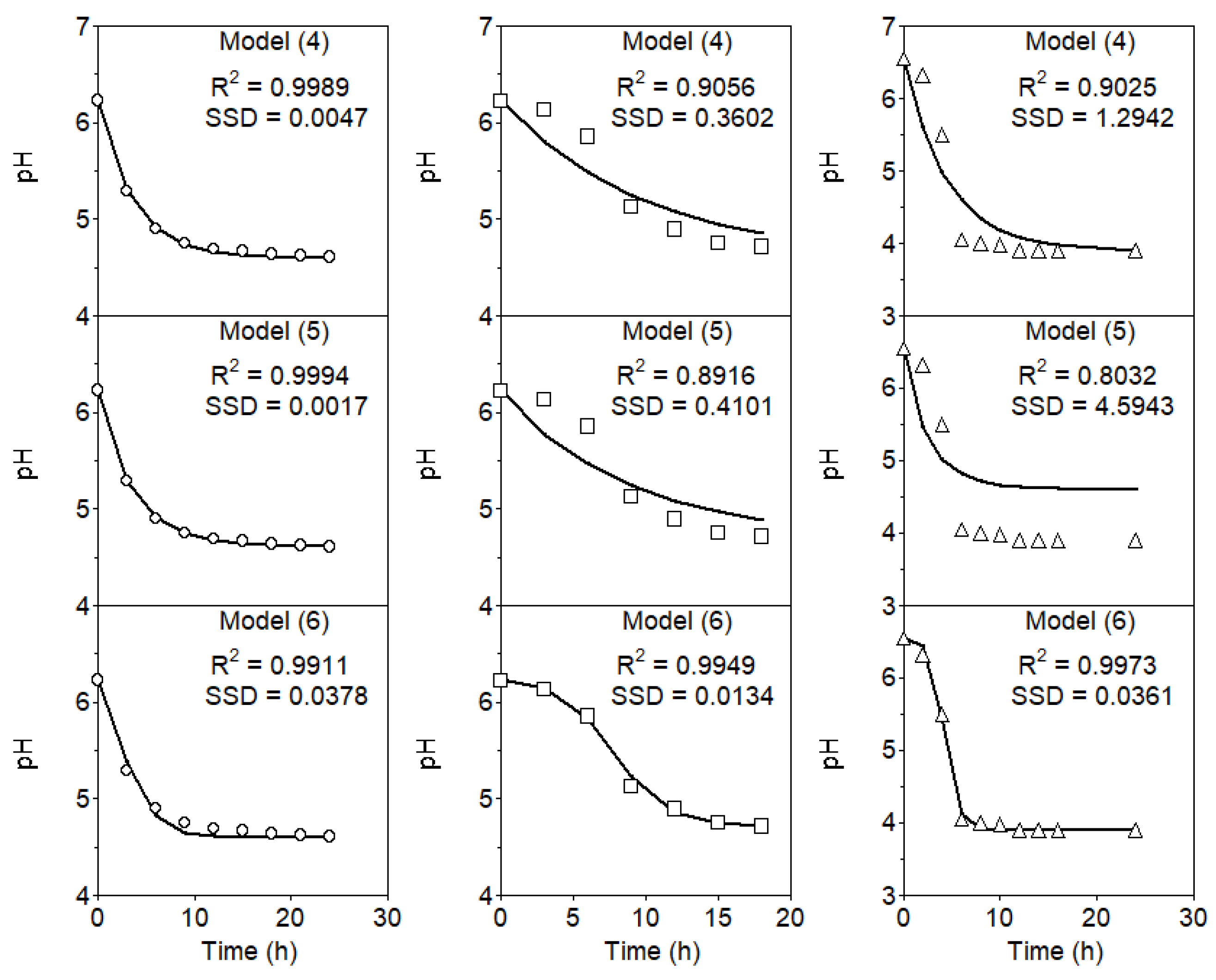
Figure 2.
Time courses of biomass (X), lactic acid (LA), total antibacterial activity (TAA), pH, total sugars (TS), and total nitrogen (TN) in batch cultures of strain CECT 539 grown in concentrated whey (closed circles) and MRS broth (open squares). The lines fitted to the experimental data (symbols) for X, LA, TAA, pH, TS, and TN were generated using models (1), (2), (3), (6), (7), and (8), respectively (A), or models (16), (17), (18), (19), (20), and (21), respectively (B).
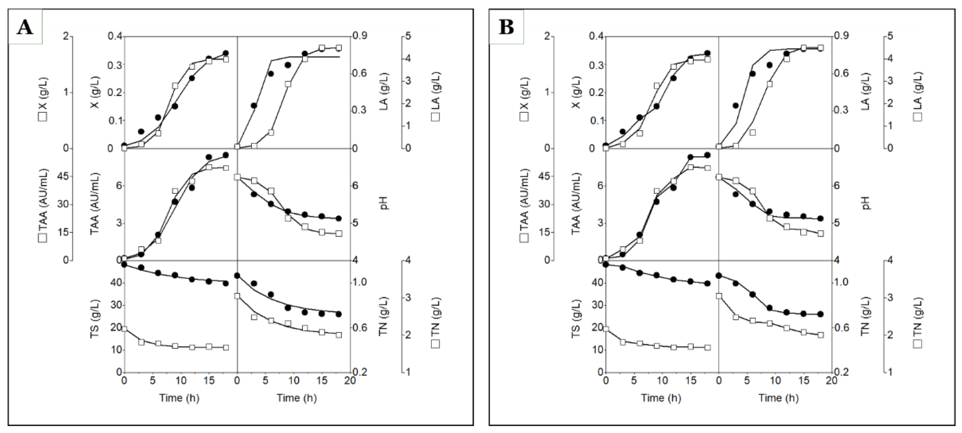
Figure 3.
Time courses of biomass (X), lactic acid (LA), total antibacterial activity (TAA), pH, total sugars (TS), and total nitrogen (TN) in batch cultures of strain CECT 539 grown in DW medium (A) and MPW medium (B), either unsupplemented (closed circles) or supplemented with glutamic acid at concentrations of 1 (open diamonds), 2 (open triangles), 3 (open squares), 4 (open inverted triangles), and 5 (open circles) g/L. Lines fitted to the experimental data (symbols) for X, LA, TAA, pH, TS, and TN were generated using models (1), (2), (3), (6), (7), and (8), respectively (A and B).

Figure 4.
Time courses of biomass (X), lactic acid (LA), total antibacterial activity (TAA), pH, total sugars (TS), and total nitrogen (TN) in batch cultures of strain CECT 539 grown in DW medium (A) and MPW medium (B), either unsupplemented (closed circles) or supplemented with glutamic acid at concentrations of 1 (open diamonds), 2 (open triangles), 3 (open squares), 4 (open inverted triangles), and 5 (open circles) g/L. Lines fitted to the experimental data (symbols) for X, LA, TAA, pH, TS, and TN were generated using models (16), (17), (18), (19), (20), and (21), respectively.
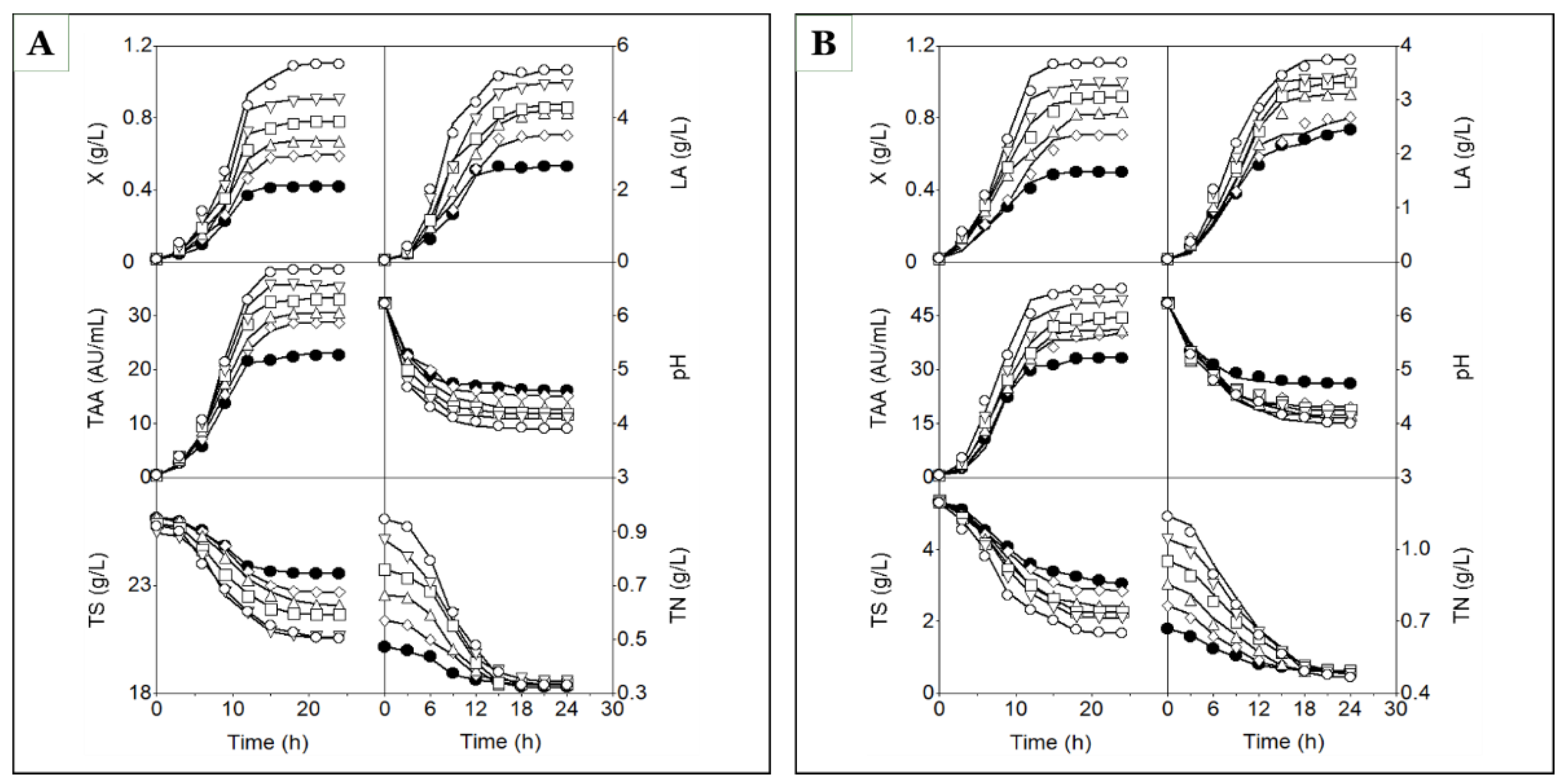
Figure 5.
Time courses of biomass (X), lactic acid (LA), total antibacterial activity (TAA), pH, total sugars (TS), and total nitrogen (TN) in batch cultures of strain CECT 539 grown in DW medium, either unsupplemented (closed circles) or supplemented with glucose at concentrations of 5 (open diamonds), 10 (open triangles), 15 (open squares), 20 (open inverted triangles), and 25 (open circles) g/L. The lines fitted to the experimental data (symbols) for X, LA, TAA, pH, TS, and TN were gener-ated using models (1), (2), (3), (6), (7), and (8), respectively (A), or models (16), (17), (18), (19), (20), and (21), respectively (B).
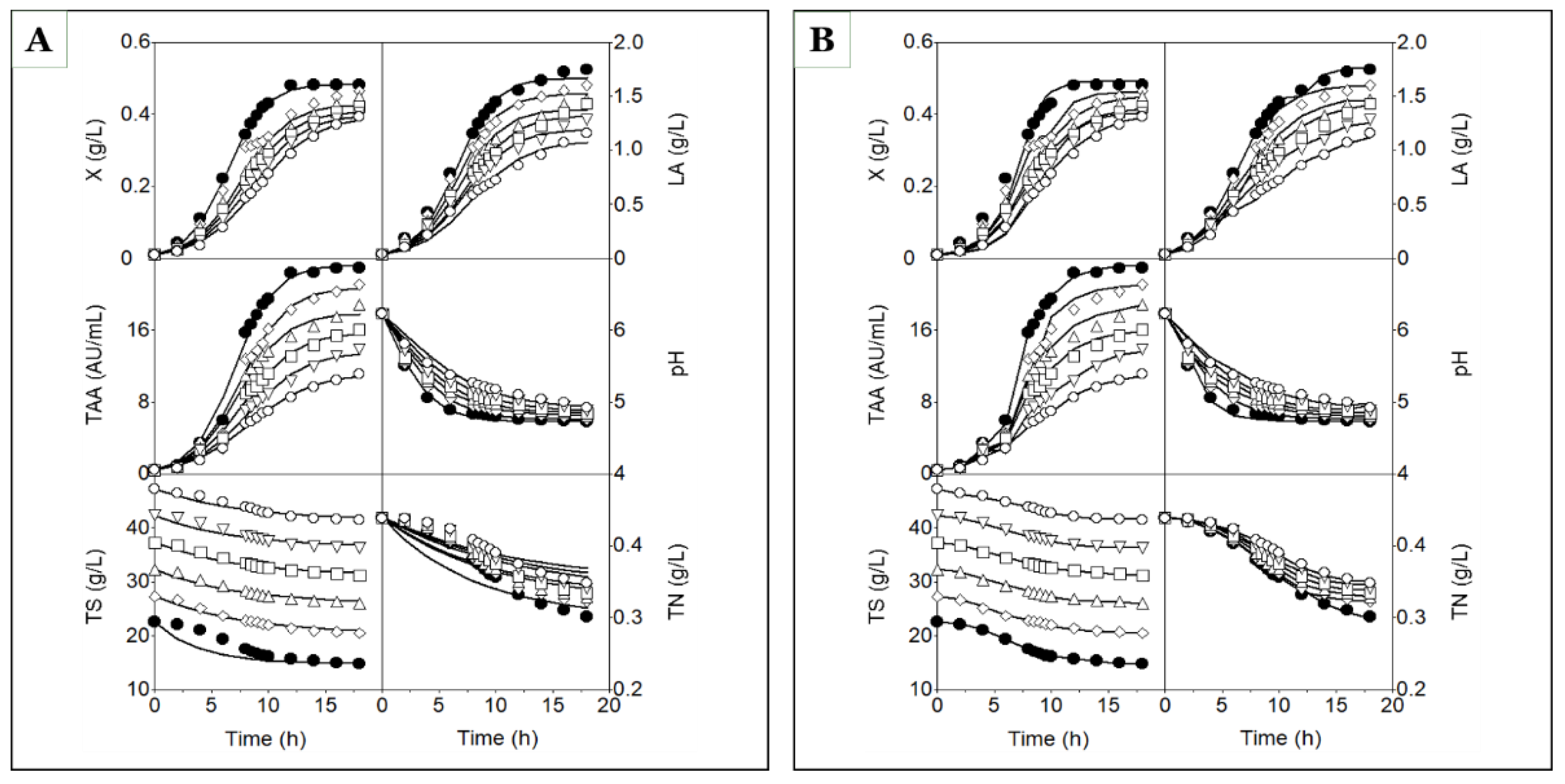
Figure 6.
Time courses of biomass (X), lactic acid (LA), total antibacterial activity (TAA), pH, total sugars (TS), and total nitrogen (TN) in batch cultures of strain CECT 4043 grown in concentrated whey (closed circles), diluted whey (open circles), and MRS broth (open squares) media. The lines fitted to the experimental data (symbols) for X, LA, TAA, pH, TS, and TN were generated using models (1), (2), (3), (6), (7), and (8), respectively (A), or models (16), (17), (18), (19), (20), and (21), respectively (B).

Figure 7.
Time courses of biomass (X), lactic acid (LA), total antibacterial activity (TAA), pH, total sugars (TS), and total nitrogen (TN) in batch cultures of strain NRRL B-5627 grown in concentrated whey (closed circles), diluted whey (open circles), and MRS broth (open squares) media. The lines fitted to the experimental data (symbols) for X, LA, TAA, pH, TS, and TN were generated using models (1), (2), (3), (6), (7), and (8), respectively (A), or models (16), (17), (18), (19), (20), and (21), respectively (B).
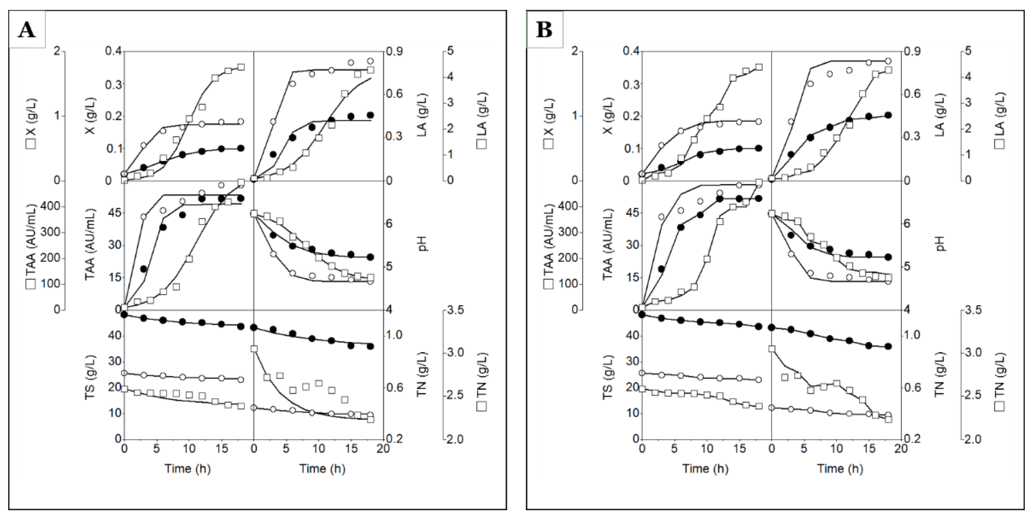
Figure 8.
Time courses of biomass (X), bacteriocin (Bact), and pH in batch cultures of Pediococcus acidilactici LB42–923 (closed circles), Lactococcus lactis subsp. lactis ATCC 11454 (open diamonds), Leuconostoc carnosum Lm1 (open triangles), and Lactobacillus sakei LB 706 (open squares) grown in TGE broth at uncontrolled pH [23]. Lines fitted to the experimental data (symbols) for X, B, and pH were generated using models (1), (3), and (6), respectively (A), or models (16), (18), and (22), respectively (B).
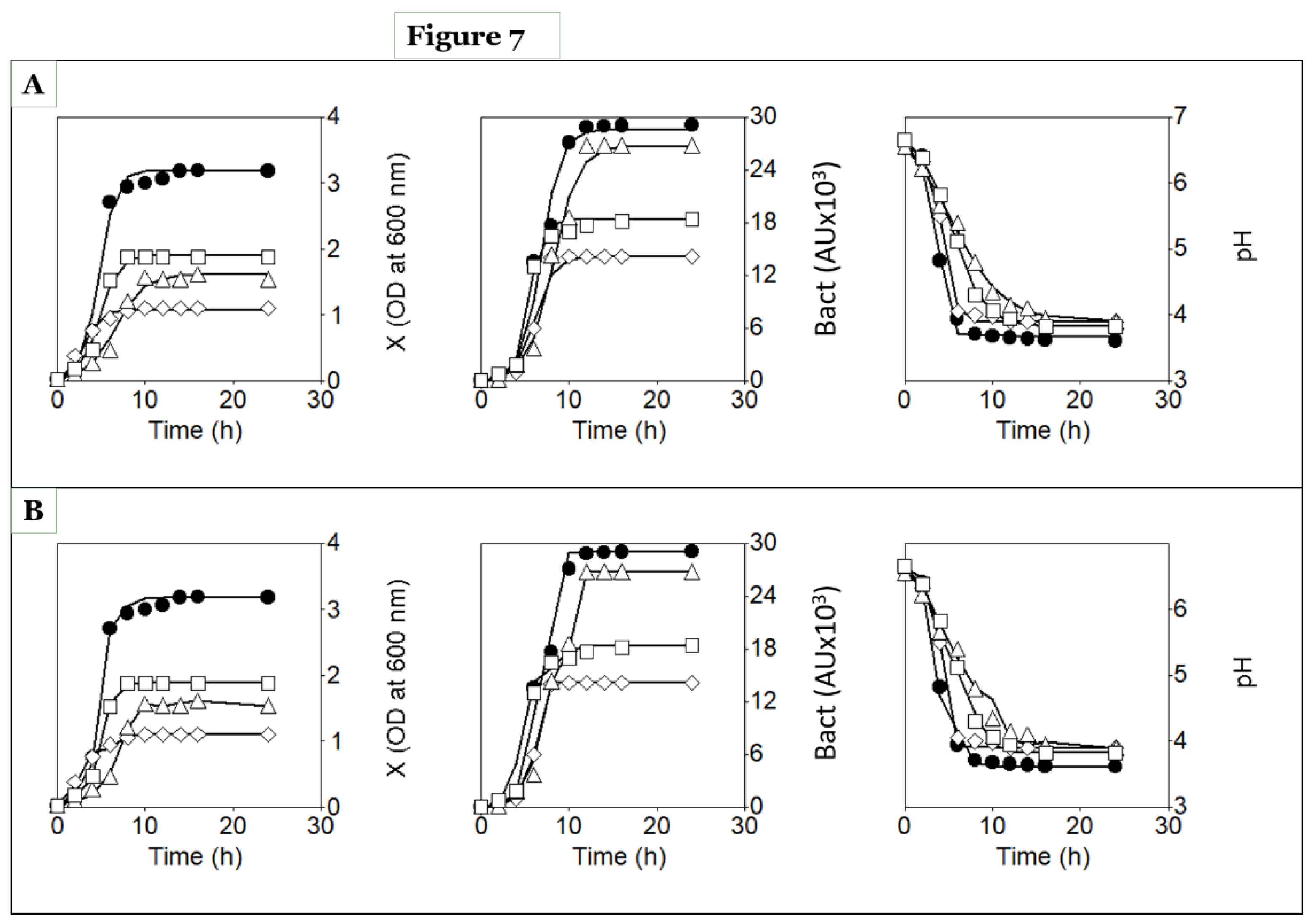

Table 1.
Mean concentrations of total sugars and total nitrogen in the culture media used for batch cultures of L. lactis CECT 539 [31,32,33,36], Lact. casei CECT 4043 [34,35], Ped. acidilactici NRRL B-5627 [31,32], Ped. acidilactici LB42–923, L. lactis subsp. lactis ATCC 11454, Leuconostoc carnosum Lm1, and Lact. sakei LB 706 [23].
| Growing Strain | Culture medium* | Total sugars (g/L) | Total nitrogen (g/L) |
|---|---|---|---|
| CECT 539, CECT 4043, NRRL B-5627 | CW | 48.11 ± 0.44 | 1.064 ± 0.018 |
| MRS | 19.59 ± 0.36 | 3.055 ± 0.005 | |
| DW | 20.54 ± 0.51 | 0.453 ± 0.014 | |
| CECT 539 | DW–GA1 | 22.16 ± 0.61 | 0.570 ± 0.030 |
| DW–GA2 | 22.19 ± 0.32 | 0.664 ± 0.011 | |
| DW–GA3 | 22.87 ± 0.17 | 0.758 ± 0.002 | |
| DW–GA4 | 22.44 ± 0.01 | 0.867 ± 0.014 | |
| DW–GA5 | 22.76 ± 0.02 | 0.945 ± 0.007 | |
| DW–G5 | 27.30 ± 0.03 | 0.439 ± 0.011 | |
| DW–G10 | 32.30 ± 0.01 | 0.439 ± 0.012 | |
| DW–G15 | 37.30 ± 0.05 | 0.438 ± 0.012 | |
| DW–G20 | 42.30 ± 0.06 | 0.438 ± 0.011 | |
| DW–G25 | 47.32 ± 0.09 | 0.436 ± 0.009 | |
| MPW | 5.33 ± 0.21 | 0.654 ± 0.009 | |
| MPW–GA1 | 5.32 ± 0.01 | 0.765 ± 0.020 | |
| MPW–GA2 | 5.32 ± 0.01 | 0.857 ± 0.012 | |
| MPW–GA3 | 5.32 ± 0.01 | 0.951 ± 0.010 | |
| MPW–GA4 | 5.31 ± 0.00 | 1.043 ± 0.022 | |
| MPW–GA5 | 5.31 ± 0.00 | 1.137 ± 0.011 | |
| LB42–923, ATCC 11454, Lm1, LB 706 | TGE | 10 ± 0.01 | 2.337 ± 0.140** |
*CW: Concentrated whey medium; MRS: de Man, Rogosa, and Sharpe broth; DW: Diluted whey medium; DW–GA1 to DW–GA5: DW medium supplemented with glutamic acid (GA) to achieve concentrations of 1, 2, 3, 4, and 5 g GA/L, respectively; DW–G5 to DW–G25: DW medium supplemented with glucose (G) to achieve concentrations of 5, 10, 15, 20, and 25 g G/L, respectively; MPW: Mussel processing waste medium; MPW–GA1 to MPW–GA5: MPW medium supplemented with glutamic acid (GA) to achieve concentrations of 1, 2, 3, 4, and 5 g GA/L, respectively; TGE: Trypticase Glucose Yeast Extract broth. **Total nitrogen was calculated in the present study, based on the TGE medium preparation described by Yang and Ray [23].
Table 2.
Estimated values for the constants of models (1), (2), (3), (6), (7), and (8), together with the coefficient of determination (R2) and the sum of squared differences (SSD) between predicted and experimental values, for the batch growth of L. lactis CECT 539 in concentrated whey (CW) medium and MRS broth.
| Culture medium | |||
| Parameter | CW medium | MRS broth | |
| KX | 0.35 | 1.60 | |
| aX | 34.19 | 336.42 | |
| bX | 0.38 | 0.73 | |
| R2X | 0.9846 | 0.9979 | |
| SSD–X | 2.29×10⁻³ | 9.20×10⁻³ | |
| KLA | 0.74 | 4.50 | |
| aLA | 44.80 | 261.64 | |
| bLA | 1.16 | 0.67 | |
| R2LA | 0.9500 | 0.9981 | |
| SSD–LA | 2.58×10⁻² | 5.05×10⁻² | |
| KTAA | 8.54 | 50.10 | |
| aTAA | 49.55 | 85.08 | |
| bTAA | 0.43 | 0.58 | |
| R2TAA | 0.9838 | 0.9856 | |
| SSD–TAA | 1.18 | 42.07 | |
| pHi | 6.23 | 6.23 | |
| pHf | 5.12 | 4.72 | |
| apH | 0.61 | 1.41×10⁻² | |
| bpH | 0.30 | 0.55 | |
| R2pH | 0.9952 | 0.9949 | |
| SSD–pH | 6.12×10⁻³ | 1.34×10⁻² | |
| TSi | 48.16 | 19.63 | |
| TSf | 39.64 | 11.11 | |
| bTS | 0.11 | 0.33 | |
| R2TS | 0.9638 | 0.9809 | |
| SSD–TS | 3.34 | 1.28 | |
| TNi | 1.07 | 3.06 | |
| TNf | 0.72 | 2.00 | |
| bTN | 0.16 | 0.17 | |
| R2TN | 0.9512 | 0.9563 | |
| SSD–TN | 8.27×10⁻³ | 3.60×10⁻² | |
R2X, R2LA, R2TAA, R2pH, R2TS, and R2TN represent the coefficients of determination for the X, LA, TAA, pH, TS, and TN models, respectively. SSD–X, SSD–LA, SSD–TAA, SSD–pH, SSD–TS, and SSD–TN correspond to the sum of squared differences for the X, LA, TAA, pH, TS, and TN models, respectively.
Table 3.
Estimated values for the constants of models (16)–(21), together with the coefficient of determination (R2) and the sum of squared differences (SSD) between predicted and experimental values, for the batch growth of L. lactis CECT 539 in concentrated whey (CW) medium and MRS broth.
Table 3.
Estimated values for the constants of models (16)–(21), together with the coefficient of determination (R2) and the sum of squared differences (SSD) between predicted and experimental values, for the batch growth of L. lactis CECT 539 in concentrated whey (CW) medium and MRS broth.
| Culture medium | |||
| Parameter | CW medium | MRS broth | |
| KX | 0.34 | 1.60 | |
| aX | 33.02 | 159.29 | |
| bpH-X | 0.29 | 0.51 | |
| R2X | 0.9962 | 0.9938 | |
| SSD–X | 6.25×10⁻⁴ | 2.07×10⁻² | |
| KLA | 0.80 | 4.50 | |
| aLA | 49.07 | 261.64 | |
| bX-LA | 0.51 | 0.67 | |
| R2LA | 0.9492 | 0.9915 | |
| SSD–LA | 3.99×10⁻² | 0.30 | |
| KTAA | 8.45 | 50.10 | |
| aTAA | 49.55 | 50.56 | |
| bX-TAA | 0.23 | 0.25 | |
| bpH-TAA | 0.12 | 0.31 | |
| R2TAA | 0.9943 | 0.9958 | |
| SSD–TAA | 0.47 | 0.12 | |
| pHi | 6.23 | 6.23 | |
| pHf | 5.12 | 4.72 | |
| apH | 0.58 | 2.20×10⁻² | |
| bLA-pH | 0.83 | 0.68 | |
| R2pH | 0.9750 | 0.9969 | |
| SSD–pH | 4.13×10⁻² | 8.43×10⁻³ | |
| TSi | 48.16 | 19.42 | |
| TSf | 39.64 | 11.11 | |
| bX-TS | 0.40 | 0.64 | |
| R2TS | 0.9926 | 0.9966 | |
| SSD–TS | 0.56 | 0.18 | |
| TNi | 1.07 | 3.06 | |
| TNf | 0.72 | 2.00 | |
| bX-TN | 0.44 | 0.63 | |
| R2TN | 0.9954 | 0.9957 | |
| SSD–TN | 8.88×10⁻⁴ | 3.57×10⁻³ | |
R2X, R2LA, R2TAA, R2pH, R2TS, and R2TN represent the coefficients of determination for the X, LA, TAA, pH, TS, and TN models, respectively. SSD–X, SSD–LA, SSD–TAA, SSD–pH, SSD–TS, and SSD–TN correspond to the sum of squared differences for the X, LA, TAA, pH, TS, and TN models, respectively.
Table 4.
Estimated values for the constants of models (1), (2), (3), (6), (7), and (8), together with the coefficient of determination (R2) and the sum of squared differences (SSD) between predicted and experimental values, for the batch growth of L. lactis CECT 539 in DW medium supplemented with different glutamic acid concentrations.
| Culture medium | ||||||
| Parameter | DW | DW–GA1 | DW–GA2 | DW–GA3 | DW–GA4 | DW–GA5 |
| KX | 0.43 | 0.61 | 0.68 | 0.79 | 0.91 | 1.09 |
| aX | 28.03 | 40.04 | 44.30 | 52.62 | 59.50 | 71.88 |
| bX | 0.39 | 0.40 | 0.43 | 0.43 | 0.45 | 0.47 |
| R2X | 0.9945 | 0.9957 | 0.9985 | 0.9966 | 0.9966 | 0.9945 |
| SSD–X | 1.460×10⁻³ | 2.135×10⁻³ | 9.76×10⁻⁴ | 3.16×10⁻³ | 4.68×10⁻³ | 1.20×10⁻² |
| KLA | 2.72 | 3.56 | 4.12 | 4.22 | 4.80 | 5.15 |
| aLA | 51.25 | 67.50 | 81.40 | 80.12 | 94.95 | 102.08 |
| bLA | 0.46 | 0.44 | 0.47 | 0.53 | 0.54 | 0.63 |
| R2LA | 0.9876 | 0.9926 | 0.9960 | 0.9948 | 0.9832 | 0.9863 |
| SSD–LA | 0.13 | 0.14 | 0.12 | 0.14 | 0.63 | 0.56 |
| KTAA | 22.82 | 28.79 | 30.42 | 32.96 | 35.57 | 38.60 |
| aTAA | 50.28 | 63.70 | 66.61 | 73.07 | 78.04 | 84.77 |
| bTAA | 0.49 | 0.48 | 0.50 | 0.52 | 0.52 | 0.53 |
| R2TAA | 0.9945 | 0.9988 | 0.9961 | 0.9971 | 0.9951 | 0.9969 |
| SSD–TAA | 3.94 | 2.15 | 6.83 | 6.67 | 11.88 | 10.02 |
| pHi | 6.23 | 6.23 | 6.23 | 6.23 | 6.23 | 6.23 |
| pHf | 4.60 | 4.50 | 4.29 | 4.18 | 4.09 | 3.90 |
| apH | 0.39 | 0.47 | 0.55 | 0.55 | 0.66 | 0.81 |
| bpH | 0.53 | 0.41 | 0.46 | 0.46 | 0.58 | 0.53 |
| R2pH | 0.9911 | 0.9796 | 0.9901 | 0.9880 | 0.9887 | 0.9871 |
| SSD–pH | 3.78×10⁻² | 6.72×10⁻² | 4.87×10⁻² | 5.42×10⁻² | 6.89×10⁻² | 9.23×10⁻² |
| TSi | 26.10 | 26.16 | 26.19 | 26.00 | 25.44 | 25.76 |
| TSf | 23.54 | 22.69 | 22.06 | 21.65 | 20.59 | 20.54 |
| bTS | 0.11 | 0.09 | 0.10 | 0.10 | 0.10 | 0.10 |
| R2TS | 0.9066 | 0.9066 | 0.9298 | 0.9460 | 0.9251 | 0.9545 |
| SSD–TS | 1.38 | 2.63 | 2.78 | 2.87 | 4.12 | 2.82 |
| TNi | 0.47 | 0.57 | 0.67 | 0.76 | 0.87 | 0.95 |
| TNf | 0.32 | 0.33 | 0.33 | 0.33 | 0.34 | 0.33 |
| bTN | 0.11 | 0.11 | 0.11 | 0.11 | 0.11 | 0.10 |
| R2TN | 0.9345 | 0.9305 | 0.9100 | 0.9041 | 0.9479 | 0.9332 |
| SSD–TN | 3.04×10⁻³ | 8.42×10⁻³ | 2.36×10⁻² | 3.91×10⁻² | 3.12×10⁻² | 5.93×10⁻² |
R2X, R2LA, R2TAA, R2pH, R2TS, and R2TN represent the coefficients of determination for the X, LA, TAA, pH, TS, and TN models, respectively. SSD–X, SSD–LA, SSD–TAA, SSD–pH, SSD–TS, and SSD–TN correspond to the sum of squared differences for the X, LA, TAA, pH, TS, and TN models, respectively.
Table 5.
Estimated values for the constants of models (1), (2), (3), (6), (7), and (8), together with the coefficient of determination (R2) and the sum of squared differences (SSD) between predicted and experimental values, for the batch growth of L. lactis CECT 539 in media prepared with mussel processing wastes supplemented with different glutamic acid concentrations.
| Culture medium | |||||||
| Parameter | MPW | MPW–GA1 | MPW–GA2 | MPW–GA3 | MPW–GA4 | MPW–GA5 | |
| KX | 0.50 | 0.71 | 0.80 | 0.90 | 0.97 | 1.10 | |
| aX | 26.40 | 38.22 | 43.76 | 48.82 | 53.00 | 60.32 | |
| bX | 0.43 | 0.39 | 0.45 | 0.47 | 0.51 | 0.52 | |
| R2X | 0.9900 | 0.9925 | 0.9797 | 0.9861 | 0.9892 | 0.9938 | |
| SSD–X | 3.98×10⁻³ | 6.73×10⁻³ | 2.10×10⁻² | 1.91×10⁻² | 1.76×10⁻² | 1.52×10⁻² | |
| KLA | 2.31 | 2.56 | 3.02 | 3.23 | 3.38 | 3.60 | |
| aLA | 47.22 | 52.42 | 61.95 | 66.38 | 69.37 | 73.94 | |
| bLA | 0.46 | 0.45 | 0.47 | 0.49 | 0.50 | 0.53 | |
| R2LA | 0.9809 | 0.9742 | 0.9798 | 0.9785 | 0.9762 | 0.9805 | |
| SSD–LA | 0.16 | 0.30 | 0.30 | 0.37 | 0.44 | 0.40 | |
| KTAA | 32.90 | 38.80 | 40.62 | 43.30 | 47.35 | 51.26 | |
| aTAA | 49.53 | 58.59 | 61.38 | 65.50 | 71.71 | 77.72 | |
| bTAA | 0.52 | 0.50 | 0.51 | 0.52 | 0.54 | 0.59 | |
| R2TAA | 0.9990 | 0.9921 | 0.9937 | 0.9870 | 0.9879 | 0.9872 | |
| SSD–TAA | 1.426 | 17.566 | 16.604 | 37.417 | 42.851 | 53.497 | |
| pHi | 6.23 | 6.23 | 6.23 | 6.17 | 6.23 | 6.23 | |
| pHf | 4.74 | 4.31 | 4.16 | 4.25 | 4.11 | 4.00 | |
| apH | 0.83 | 0.64 | 0.64 | 0.88 | 0.53 | 0.92 | |
| bpH | 0.41 | 0.33 | 0.33 | 0.30 | 0.28 | 0.24 | |
| R2pH | 0.9830 | 0.9755 | 0.9800 | 0.9762 | 0.9772 | 0.9868 | |
| SSD–pH | 5.33×10⁻² | 0.11 | 9.50×10⁻² | 9.79×10⁻² | 0.13 | 7.46×10⁻² | |
| TSi | 5.32 | 5.32 | 5.32 | 5.36 | 5.31 | 5.31 | |
| TSf | 3.05 | 2.84 | 2.41 | 2.26 | 2.00 | 1.67 | |
| bTS | 0.10 | 0.10 | 0.11 | 0.12 | 0.11 | 0.13 | |
| R2TS | 0.9662 | 0.9682 | 0.9614 | 0.9693 | 0.9719 | 0.9765 | |
| SSD–TS | 0.37 | 0.50 | 0.69 | 0.61 | 0.55 | 0.56 | |
| TNi | 0.67 | 0.77 | 0.86 | 0.95 | 1.04 | 1.14 | |
| TNf | 0.49 | 0.49 | 0.49 | 0.49 | 0.48 | 0.47 | |
| bTN | 0.11 | 0.11 | 0.12 | 0.10 | 0.10 | 0.11 | |
| R2TN | 0.9846 | 0.9846 | 0.9767 | 0.9701 | 0.9649 | 0.9645 | |
| SSD–TN | 1.70×10⁻³ | 4.21×10⁻³ | 5.84×10⁻³ | 1.31×10⁻² | 2.38×10⁻² | 3.46×10⁻² | |
R2X, R2LA, R2TAA, R2pH, R2TS, and R2TN represent the coefficients of determination for the X, LA, TAA, pH, TS, and TN models, respectively. SSD–X, SSD–LA, SSD–TAA, SSD–pH, SSD–TS, and SSD–TN correspond to the sum of squared differences for the X, LA, TAA, pH, TS, and TN models, respectively.
Table 6.
Estimated values for the constants of models (16), (17), (18), (19), (20), and (21), together with the coefficient of determination (R2) and the sum of squared differences (SSD) between predicted and experimental values, for the batch growth of L. lactis CECT 539 in diluted whey medium supplemented with different glutamic acid concentrations.
| Culture medium | ||||||
| Parameter | DW | DW–GA1 | DW–GA2 | DW–GA3 | DW–GA4 | DW–GA5 |
| KX | 0.42 | 0.60 | 0.67 | 0.78 | 0.90 | 1.11 |
| aX | 27.59 | 39.51 | 46.31 | 51.81 | 60.13 | 73.89 |
| bpH-X | 0.28 | 0.25 | 0.24 | 0.29 | 0.31 | 0.27 |
| R2X | 0.9984 | 0.9975 | 0.9955 | 0.9899 | 0.9872 | 0.9941 |
| SSD–X | 7.91×10⁻⁴ | 1.32×10⁻³ | 4.23×10⁻³ | 1.09×10⁻² | 1.98×10⁻² | 1.69×10⁻² |
| KLA | 2.66 | 3.54 | 4.20 | 4.38 | 4.97 | 5.34 |
| aLA | 50.26 | 67.04 | 79.74 | 83.32 | 94.59 | 101.78 |
| bX-LA | 0.38 | 0.40 | 0.45 | 0.43 | 0.49 | 0.47 |
| R2LA | 0.9972 | 0.9949 | 0.9946 | 0.9963 | 0.9873 | 0.9918 |
| SSD–LA | 3.97×10⁻² | 9.83×10⁻² | 0.13 | 0.13 | 0.52 | 0.435 |
| KTAA | 23.19 | 28.69 | 30.61 | 33.61 | 35.89 | 38.89 |
| aTAA | 51.11 | 63.47 | 67.78 | 74.53 | 79.65 | 86.39 |
| bX-TAA | 0.25 | 0.20 | 0.34 | 0.28 | 0.31 | 0.30 |
| bpH-TAA | 0.10 | 0.13 | 5.73×10⁻² | 0.11 | 0.10 | 0.10 |
| R2TAA | 0.9991 | 0.9989 | 0.9986 | 0.9979 | 0.9949 | 0.9959 |
| SSD–TAA | 0.68 | 1.37 | 2.18 | 5.21 | 12.88 | 15.01 |
| pHi | 6.23 | 6.23 | 6.23 | 6.23 | 6.23 | 6.23 |
| pHf | 4.60 | 4.50 | 4.26 | 4.17 | 4.08 | 3.90 |
| apH | 4.31 | 4.31 | 4.31 | 4.31 | 4.31 | 4.31 |
| bLA-pH | 0.48 | 0.49 | 0.49 | 0.55 | 0.61 | 0.68 |
| R2pH | 0.9949 | 0.9976 | 0.9968 | 0.9993 | 0.9978 | 0.9976 |
| SSD–pH | 1.16×10⁻² | 7.02×10⁻³ | 1.32×10⁻² | 3.70×10⁻³ | 1.17×10⁻² | 1.64×10⁻² |
| TSi | 26.16 | 26.16 | 26.20 | 25.88 | 25.45 | 25.78 |
| TSf | 23.55 | 22.68 | 22.01 | 21.63 | 20.59 | 20.54 |
| bX-TS | 0.41 | 0.42 | 0.41 | 0.41 | 0.47 | 0.47 |
| R2TS | 0.9982 | 0.9988 | 0.9986 | 0.9992 | 0.9993 | 0.9988 |
| SSD–TS | 1.86×10⁻² | 2.29×10⁻² | 7.63×10⁻² | 4.94×10⁻² | 2.63×10⁻² | 6.19×10⁻² |
| TNi | 0.47 | 0.57 | 0.67 | 0.76 | 0.87 | 0.95 |
| TNf | 0.32 | 0.33 | 0.33 | 0.33 | 0.35 | 0.33 |
| bX-TN | 0.43 | 0.42 | 0.43 | 0.43 | 0.50 | 0.50 |
| R2TN | 0.9973 | 0.9985 | 1.0000 | 0.9997 | 0.9981 | 0.9987 |
| SSD–TN | 1.00×10⁻⁴ | 1.21×10⁻⁴ | 2.89×10⁻⁵ | 1.55×10⁻⁴ | 8.66×10⁻⁴ | 9.60×10⁻⁴ |
R2X, R2LA, R2TAA, R2pH, R2TS, and R2TN represent the coefficients of determination for the X, LA, TAA, pH, TS, and TN models, respectively. SSD–X, SSD–LA, SSD–TAA, SSD–pH, SSD–TS, and SSD–TN correspond to the sum of squared differences for the X, LA, TAA, pH, TS, and TN models, respectively.
Table 7.
Estimated values for the constants of models (16), (17), (18), (19), (20), and (21), together with the coefficient of determination (R2) and the sum of squared differences (SSD) between predicted and experimental values, for the batch growth of L. lactis CECT 539 in media prepared with mussel processing wastes supplemented with different glutamic acid concentrations.
| Culture medium | ||||||
| Parameter | MPW | MPW–GA1 | MPW–GA2 | MPW–GA3 | MPW–GA4 | MPW–GA5 |
| KX | 0.50 | 0.71 | 0.83 | 0.92 | 1.00 | 1.11 |
| aX | 26.72 | 38.26 | 45.42 | 50.20 | 54.39 | 60.78 |
| bpH-X | 0.37 | 0.21 | 0.21 | 0.20 | 0.18 | 0.18 |
| R2X | 0.9920 | 0.9919 | 0.9968 | 0.9913 | 0.9886 | 0.9940 |
| SSD–X | 3.33×10⁻³ | 7.19×10⁻³ | 3.38×10⁻³ | 1.16×10⁻² | 1.74×10⁻² | 1.31×10⁻² |
| KLA | 2.46 | 2.67 | 3.11 | 3.32 | 3.48 | 3.75 |
| aLA | 50.22 | 54.74 | 63.80 | 63.80 | 71.61 | 77.13 |
| bX-LA | 0.63 | 0.40 | 0.44 | 0.44 | 0.48 | 0.49 |
| R2LA | 0.9884 | 0.9780 | 0.9820 | 0.9856 | 0.9878 | 0.9942 |
| SSD–LA | 0.10 | 0.21 | 0.312 | 0.33 | 0.28 | 0.16 |
| KTAA | 33.32 | 40.19 | 41.19 | 44.60 | 49.16 | 52.56 |
| aTAA | 50.17 | 60.72 | 62.25 | 67.49 | 74.49 | 79.71 |
| bX-TAA | 0.63 | 0.27 | 0.21 | 0.00 | 0.24 | 0.08 |
| bpH-TAA | 2.55×10⁻³ | 6.85×10⁻² | 0.10 | 0.19 | 8.87×10⁻² | 0.15 |
| R2TAA | 0.9951 | 0.9923 | 0.9954 | 0.9947 | 0.9898 | 0.9939 |
| SSD–TAA | 10.13 | 20.07 | 18.59 | 16.86 | 43.64 | 28.68 |
| pHi | 6.23 | 6.23 | 6.23 | 6.23 | 6.23 | 6.23 |
| pHf | 4.74 | 4.30 | 4.14 | 4.23 | 4.10 | 3.98 |
| apH | 4.31 | 4.31 | 4.31 | 4.31 | 4.31 | 4.31 |
| bLA-pH | 0.82 | 0.55 | 0.55 | 0.55 | 0.54 | 0.56 |
| R2pH | 0.9924 | 0.9760 | 0.9917 | 0.9887 | 0.9868 | 0.9890 |
| SSD–pH | 2.11×10⁻² | 0.11 | 4.38×10⁻² | 5.32×10⁻² | 7.54×10⁻² | 7.23×10⁻² |
| TSi | 5.32 | 5.32 | 5.32 | 5.32 | 5.31 | 5.31 |
| TSf | 3.05 | 2.84 | 2.41 | 2.26 | 2.09 | 1.67 |
| bX-TS | 0.64 | 0.41 | 0.41 | 0.41 | 0.41 | 0.46 |
| R2TS | 0.9981 | 0.9969 | 0.9963 | 0.9947 | 0.9938 | 0.9964 |
| SSD–TS | 1.51×10⁻² | 2.98×10⁻² | 7.97×10⁻² | 0.11 | 0.21 | 0.12 |
| TNi | 0.67 | 0.77 | 0.86 | 0.95 | 1.05 | 1.14 |
| TNf | 0.49 | 0.49 | 0.49 | 0.49 | 0.48 | 0.47 |
| bX-TN | 0.69 | 0.43 | 0.43 | 0.43 | 0.43 | 0.43 |
| R2TN | 0.9961 | 0.9958 | 0.9942 | 0.9966 | 0.9968 | 0.9963 |
| SSD–TN | 1.92×10⁻⁴ | 4.82×10⁻⁴ | 1.53×10⁻³ | 1.76×10⁻³ | 3.37×10⁻³ | 4.88×10⁻³ |
R2X, R2LA, R2TAA, R2pH, R2TS, and R2TN represent the coefficients of determination for the X, LA, TAA, pH, TS, and TN models, respectively. SSD–X, SSD–LA, SSD–TAA, SSD–pH, SSD–TS, and SSD–TN correspond to the sum of squared differences for the X, LA, TAA, pH, TS, and TN models, respectively.
Table 8.
Estimated values for the constants of models (1), (2), (3), (6), (7), and (8), together with the coefficient of determination (R2) and the sum of squared differences (SSD) between predicted and experimental values, for the batch growth of L. lactis CECT 539 in diluted whey medium supplemented with different glucose concentrations.
| Culture medium | ||||||
| Parameter | DW | DW–G5 | DW–G10 | DW–G15 | DW–G20 | DW–G25 |
| KX | 0.48 | 0.48 | 0.43 | 0.41 | 0.40 | 0.39 |
| aX | 47.42 | 47.42 | 41.84 | 39.99 | 38.98 | 38.35 |
| bX | 0.60 | 0.60 | 0.49 | 0.47 | 0.44 | 0.40 |
| R2X | 0.9984 | 0.9727 | 0.9917 | 0.9962 | 0.9985 | 0.9973 |
| SSD–X | 8.10×10⁻⁴ | 4.06×10⁻² | 2.61×10⁻³ | 9.99×10⁻⁴ | 3.22×10⁻⁴ | 5.70×10⁻⁴ |
| KLA | 1.67 | 1.52 | 1.38 | 1.33 | 1.20 | 1.08 |
| aLA | 46.98 | 42.71 | 38.63 | 37.06 | 33.26 | 30.10 |
| bLA | 0.59 | 0.56 | 0.53 | 0.48 | 0.48 | 0.43 |
| R2LA | 0.9926 | 0.9874 | 0.9865 | 0.9784 | 0.9821 | 0.9808 |
| SSD–LA | 4.28×10⁻² | 5.70×10⁻² | 4.41×10⁻² | 6.21×10⁻² | 4.19×10⁻² | 3.31×10⁻² |
| KTAA | 23.27 | 20.71 | 17.87 | 15.69 | 13.58 | 11.11 |
| aTAA | 50.76 | 44.16 | 37.98 | 33.22 | 28.61 | 23.24 |
| bTAA | 0.56 | 0.50 | 0.49 | 0.45 | 0.40 | 0.37 |
| R2TAA | 0.9922 | 0.9901 | 0.9883 | 0.9931 | 0.9868 | 0.9948 |
| SSD–TAA | 7.70 | 6.63 | 5.90 | 2.39 | 3.21 | 0.86 |
| pHi | 6.23 | 6.23 | 6.23 | 6.23 | 6.20 | 6.23 |
| pHf | 4.73 | 4.76 | 4.81 | 4.84 | 4.87 | 4.92 |
| apH | 0.93 | 0.79 | 0.92 | 0.87 | 0.68 | 0.67 |
| bpH | 0.50 | 0.40 | 0.34 | 0.32 | 0.29 | 0.26 |
| R2pH | 0.9951 | 0.9798 | 0.9747 | 0.9668 | 0.9699 | 0.9822 |
| SSD–pH | 2.09×10⁻² | 7.21×10⁻² | 7.67×10⁻² | 9.25×10⁻² | 7.29×10⁻² | 4.65×10⁻² |
| TSi | 22.63 | 27.46 | 32.36 | 37.36 | 42.32 | 47.32 |
| TSf | 14.84 | 20.50 | 26.00 | 31.23 | 36.29 | 41.47 |
| bTS | 0.26 | 0.14 | 0.14 | 0.14 | 0.14 | 0.14 |
| R2TS | 0.8194 | 0.9758 | 0.9691 | 0.9683 | 0.9503 | 0.9425 |
| SSD–TS | 36.16 | 2.32 | 2.52 | 2.40 | 4.04 | 3.77 |
| TNi | 0.44 | 0.44 | 0.44 | 0.44 | 0.44 | 0.44 |
| TNf | 0.30 | 0.32 | 0.33 | 0.33 | 0.34 | 0.35 |
| bTN | 0.12 | 0.10 | 0.10 | 0.08 | 0.08 | 0.08 |
| R2TN | 0.8766 | 0.9192 | 0.9180 | 0.9209 | 0.9069 | 0.8793 |
| SSD–TN | 6.21×10⁻³ | 2.62×10⁻³ | 2.32×10⁻³ | 2.46×10⁻³ | 2.16×10⁻³ | 2.30×10⁻³ |
R2X, R2LA, R2TAA, R2pH, R2TS, and R2TN represent the coefficients of determination for the X, LA, TAA, pH, TS, and TN models, respectively. SSD–X, SSD–LA, SSD–TAA, SSD–pH, SSD–TS, and SSD–TN correspond to the sum of squared differences for the X, LA, TAA, pH, TS, and TN models, respectively.
Table 9.
Estimated values for the constants of models (16), (17), (18), (19), (20), and (21), together with the coefficient of determination (R2) and the sum of squared differences (SSD) between predicted and experimental values, for the batch growth of L. lactis CECT 539 in diluted whey medium supplemented with different glucose concentrations.
| Culture medium | ||||||
| Parameter | DW | DW–G5 | DW–G10 | DW–G15 | DW–G20 | DW–G25 |
| KX | 0.49 | 0.47 | 0.45 | 0.42 | 0.40 | 0.39 |
| aX | 48.43 | 45.54 | 44.04 | 41.01 | 39.40 | 38.30 |
| bpH-X | 0.58 | 0.37 | 0.31 | 0.27 | 0.36 | 0.23 |
| R2X | 0.9824 | 0.9847 | 0.9873 | 0.9938 | 0.9893 | 0.9960 |
| SSD–X | 1.27×10⁻² | 8.05×10⁻³ | 6.42×10⁻³ | 2.49×10⁻³ | 4.66×10⁻³ | 1.37×10⁻³ |
| KLA | 1.76 | 1.61 | 1.49 | 1.43 | 1.28 | 1.16 |
| aLA | 49.57 | 45.05 | 41.61 | 41.61 | 35.69 | 32.25 |
| bX-LA | 0.60 | 0.53 | 0.48 | 0.48 | 0.43 | 0.40 |
| R2LA | 0.9970 | 0.9862 | 0.9894 | 0.9922 | 0.9972 | 0.9921 |
| SSD–LA | 2.17×10⁻² | 7.89×10⁻² | 5.02×10⁻² | 4.86×10⁻² | 5.27×10⁻³ | 1.35×10⁻² |
| KTAA | 23.12 | 21.12 | 18.82 | 16.07 | 13.86 | 11.16 |
| aTAA | 50.42 | 45.05 | 40.04 | 34.13 | 29.22 | 23.33 |
| bX-TAA | 0.59 | 0.51 | 0.47 | 0.47 | 0.43 | 0.40 |
| bpH-TAA | 1.89×10⁻³ | 2.00×10⁻³ | 2.46×10⁻³ | 2.00×10⁻³ | 2.00×10⁻³ | 2.00×10⁻³ |
| R2TAA | 0.9993 | 0.9890 | 0.9941 | 0.9964 | 0.9983 | 0.9970 |
| SSD–TAA | 1.07 | 10.61 | 5.25 | 2.11 | 0.45 | 0.50 |
| pHi | 6.23 | 6.23 | 6.23 | 6.23 | 6.23 | 6.23 |
| pHf | 4.73 | 4.76 | 4.80 | 4.84 | 4.87 | 4.92 |
| apH | 0.14 | 0.48 | 0.68 | 1.00 | 0.19 | 0.84 |
| bLA-pH | 0.73 | 0.62 | 0.55 | 0.53 | 0.50 | 0.44 |
| R2pH | 0.9855 | 0.9795 | 0.9852 | 0.9804 | 0.9648 | 0.9839 |
| SSD–pH | 6.03×10⁻² | 7.10×10⁻² | 4.63×10⁻² | 5.32×10⁻² | 9.05×10⁻² | 3.61×10⁻² |
| TSi | 22.63 | 27.46 | 32.36 | 37.36 | 42.32 | 47.32 |
| TSf | 14.83 | 20.50 | 26.00 | 31.23 | 36.29 | 41.47 |
| bX-TS | 0.60 | 0.53 | 0.48 | 0.46 | 0.46 | 0.41 |
| R2TS | 0.9995 | 0.9972 | 0.9978 | 0.9989 | 0.9989 | 0.9976 |
| SSD–TS | 9.46×10⁻² | 0.36 | 0.23 | 8.80×10⁻² | 0.12 | 0.16 |
| TNi | 0.44 | 0.44 | 0.44 | 0.44 | 0.44 | 0.44 |
| TNf | 0.30 | 0.32 | 0.33 | 0.33 | 0.34 | 0.35 |
| bX-TN | 0.54 | 0.54 | 0.47 | 0.47 | 0.47 | 0.45 |
| R2TN | 0.9963 | 0.9975 | 0.9989 | 0.9976 | 0.9955 | 0.9960 |
| SSD–TN | 1.87×10⁻⁴ | 1.01×10⁻⁴ | 4.10×10⁻⁵ | 3.97×10⁻⁵ | 8.38×10⁻⁵ | 9.86×10⁻⁵ |
R2X, R2LA, R2TAA, R2pH, R2TS, and R2TN represent the coefficients of determination for the X, LA, TAA, pH, TS, and TN models, respectively. SSD–X, SSD–LA, SSD–TAA, SSD–pH, SSD–TS, and SSD–TN correspond to the sum of squared differences for the X, LA, TAA, pH, TS, and TN models, respectively.
Table 10.
Estimated values for the constants of models (1), (2), (3), (6), (7), and (8), together with the coefficient of determination (R²) and the sum of squared differences (SSD) between predicted and experimental values, for the batch growth of Lact. casei CECT 4043 and Pediococcus acidilactici NRRL B–562 in concentrated whey (CW), diluted whey (DW), and MRS broth.
| Culture medium/Strain | ||||||
|---|---|---|---|---|---|---|
| Parameter | CW/CECT 4043 | DW/CECT 4043 | MRS/CECT 4043 | CW/NRRL B–562 | DW/NRRL B–562 | MRS/NRRL B–562 |
| KX | 0.18 | 0.33 | 2.22 | 0.10 | 0.17 | 1.77 |
| aX | 21.76 | 15.69 | 221.37 | 4.08 | 7.69 | 176.40 |
| bX | 0.26 | 0.45 | 0.49 | 0.30 | 0.81 | 0.52 |
| R2X | 0.9676 | 0.9909 | 0.9758 | 0.9990 | 0.9836 | 0.9854 |
| SSD–X | 1.05×10⁻³ | 1.02×10⁻³ | 0.20 | 6.40×10⁻⁶ | 3.43×10⁻⁴ | 8.60×10⁻² |
| KLA | 1.33 | 2.17 | 22.56 | 0.42 | 0.77 | 4.28 |
| aLA | 44.29 | 47.71 | 50.63 | 45.05 | 45.38 | 50.08 |
| bLA | 0.33 | 0.63 | 0.30 | 0.88 | 1.29 | 0.36 |
| R2LA | 0.9597 | 0.9861 | 0.9982 | 0.9346 | 0.9734 | 0.9853 |
| SSD–LA | 8.26×10⁻² | 7.51×10⁻² | 0.87 | 1.25×10⁻² | 1.42×10⁻² | 0.48 |
| KTAA | 1.84 | 3.00 | 11.98 | 49.03 | 53.25 | 526.10 |
| aTAA | 43.60 | 42.81 | 49.02 | 46.88 | 45.07 | 53.40 |
| bTAA | 0.34 | 0.73 | 0.38 | 0.95 | 1.75 | 0.36 |
| R2TAA | 0.9708 | 0.9884 | 0.9905 | 0.9648 | 0.9563 | 0.9859 |
| SSD–TAA | 0.10 | 0.15 | 1.58 | 88.98 | 103.37 | 4417.13 |
| pHi | 7.02 | 7.01 | 6.42 | 6.23 | 6.23 | 6.23 |
| pHf | 5.38 | 4.34 | 4.39 | 5.22 | 4.66 | 4.68 |
| apH | 0.27 | 0.52 | 0.27 | 0.99 | 0.37 | 6.66×10⁻² |
| bpH | 0.31 | 0.26 | 0.24 | 0.31 | 0.60 | 0.34 |
| R2pH | 0.9947 | 0.9935 | 0.9941 | 0.9881 | 0.9950 | 0.9968 |
| SSD–pH | 1.44×10⁻² | 4.43×10⁻² | 3.59×10⁻² | 1.26×10⁻² | 2.39×10⁻² | 9.77×10⁻³ |
| TSi | 48.18 | 22.56 | 20.32 | 48.18 | 25.58 | 19.63 |
| TSf | 44.43 | 17.17 | 6.33 | 43.60 | 23.00 | 12.85 |
| bTS | 8.36×10⁻² | 0.16 | 8.57×10⁻² | 0.11 | 0.11 | 0.13 |
| R2TS | 0.9515 | 0.9731 | 0.8823 | 0.9661 | 0.9684 | 0.6789 |
| SSD–TS | 1.23 | 0.92 | 29.48 | 0.48 | 0.16 | 23.89 |
| TNi | 1.19 | 0.48 | 3.33 | 1.06 | 0.44 | 3.06 |
| TNf | 1.00 | 0.34 | 2.68 | 0.92 | 0.39 | 2.22 |
| bTN | 0.05 | 0.15 | 0.08 | 0.10 | 0.12 | 0.24 |
| R2TN | 0.9790 | 0.9467 | 0.9336 | 0.9365 | 0.9491 | 0.7400 |
| SSD–TN | 1.35×10⁻³ | 1.20×10⁻³ | 4.66×10⁻² | 1.93×10⁻³ | 1.76×10⁻⁴ | 0.40 |
R2X, R2LA, R2TAA, R2pH, R2TS, and R2TN represent the coefficients of determination for the X, LA, TAA, pH, TS, and TN models, respectively. SSD–X, SSD–LA, SSD–TAA, SSD–pH, SSD–TS, and SSD–TN correspond to the sum of squared differences for the X, LA, TAA, pH, TS, and TN models, respectively.
Table 11.
Estimated parameter values for models (16), (17), (18), (19), (20), and (21), together with the coefficient of determination (R²) and the sum of squared differences (SSD) between predicted and experimental values, for the batch growth of Lact. casei CECT 4043 and Pediococcus acidilactici NRRL B–562 in concentrated whey (CW), diluted whey (DW), and MRS broth.
| Culture medium/Strain | ||||||
| Parameter | CW/CECT 4043 | DW/CECT 4043 | MRS/CECT 4043 | CW/NRRL B–562 | DW/NRRL B–562 | MRS/NRRL B–562 |
| KX | 0.21 | 0.34 | 2.22 | 0.10 | 0.18 | 1.76 |
| aX | 25.52 | 15.90 | 221.30 | 4.03 | 8.19 | 175.01 |
| bpH-X | 0.22 | 0.97 | 0.22 | 0.32 | 0.49 | 0.41 |
| R2X | 0.9951 | 0.9825 | 0.9961 | 0.9883 | 0.9916 | 0.9955 |
| SSD–X | 2.20×10⁻⁴ | 2.89×10⁻³ | 2.39×10⁻² | 1.05×10⁻⁴ | 3.07×10⁻⁴ | 1.96×10⁻² |
| KLA | 1.47 | 2.23 | 21.89 | 0.45 | 0.83 | 4.28 |
| aLA | 49.06 | 47.71 | 49.10 | 49.07 | 49.06 | 50.08 |
| bX-LA | 0.25 | 0.46 | 0.45 | 0.31 | 0.77 | 0.51 |
| R2LA | 0.9643 | 0.9901 | 0.9910 | 0.9944 | 0.9746 | 0.9936 |
| SSD–LA | 0.10 | 5.85×10⁻² | 7.21 | 9.51×10⁻⁴ | 2.66×10⁻² | 0.18 |
| KTAA | 2.08 | 3.14 | 11.98 | 51.70 | 57.93 | 493.32 |
| aTAA | 23.30 | 43.47 | 49.05 | 49.49 | 49.11 | 50.01 |
| bX-TAA | 2.07×10⁻³ | 0.44 | 1.62×10⁻² | 0.28 | 0.73 | 0.13 |
| bpH-TAA | 0.21 | 1.25×10⁻³ | 0.21 | 3.12×10⁻² | 2.30×10⁻² | 0.31 |
| R2TAA | 0.9972 | 0.9840 | 0.9979 | 0.9964 | 0.9609 | 0.9963 |
| SSD–TAA | 1.0×10⁻² | 0.18 | 0.44 | 9.95 | 143.32 | 1182.13 |
| pHi | 7.00 | 7.00 | 6.42 | 6.23 | 6.23 | 6.23 |
| pHf | 5.37 | 4.34 | 4.39 | 5.22 | 4.66 | 4.75 |
| apH | 0.71 | 0.86 | 0.36 | 0.59 | 0.71 | 3.83×10⁻² |
| bLA-pH | 0.31 | 0.57 | 0.31 | 0.80 | 1.16 | 0.36 |
| R2pH | 0.9910 | 0.9863 | 0.9975 | 0.9659 | 0.9902 | 0.9889 |
| SSD–pH | 2.85×10⁻² | 8.64×10⁻² | 1.13×10⁻² | 4.17×10⁻² | 4.12×10⁻² | 4.10×10⁻² |
| TSi | 48.18 | 22.56 | 20.32 | 48.18 | 25.58 | 19.63 |
| TSf | 44.43 | 17.17 | 6.33 | 43.60 | 23.00 | 12.85 |
| bX-TS | 0.24 | 0.41 | 0.46 | 0.30 | 0.48 | 0.60 |
| R2TS | 0.9833 | 0.9582 | 0.9973 | 0.9988 | 0.9828 | 0.9867 |
| SSD–TS | 0.24 | 0.84 | 1.32 | 1.76×10⁻² | 0.14 | 0.80 |
| TNi | 1.19 | 0.48 | 3.33 | 1.06 | 0.44 | 3.06 |
| TNf | 1.00 | 0.34 | 2.68 | 0.92 | 0.39 | 2.22 |
| bX-TN | 0.23 | 0.45 | 0.49 | 0.30 | 0.48 | 0.54 |
| R2TN | 0.9886 | 0.9922 | 0.9952 | 0.9997 | 0.9918 | 0.9693 |
| SSD–TN | 5.00×10⁻⁴ | 1.67×10⁻⁴ | 2.60×10⁻³ | 7.14×10⁻⁶ | 4.50×10⁻⁵ | 2.27×10⁻² |
R2X, R2LA, R2TAA, R2pH, R2TS, and R2TN represent the coefficients of determination for the X, LA, TAA, pH, TS, and TN models, respectively. SSD–X, SSD–LA, SSD–TAA, SSD–pH, SSD–TS, and SSD–TN correspond to the sum of squared differences for the X, LA, TAA, pH, TS, and TN models, respectively.
Table 12.
Estimated parameter values for models (1), (3), and (6), together with the coefficient of determination (R²) and the sum of squared differences (SSD) between predicted and experimental values, for the batch growth of Pediococcus acidilactici LB42–923, Lactococcus lactis subsp. lactis ATCC 11454, Leuconostoc carnosum Lm1, and Lactobacillus sakei LB 706 in concentrated TGE broth.
| Strain | |||||
| Parameter | LB42–923 | ATCC 11454 | Lm1 | LB 706 | |
| KX | 3.19 | 1.08 | 1.61 | 1.91 | |
| aX | 155.53 | 34.86 | 58.70 | 100.37 | |
| bX | 1.07 | 1.15 | 0.62 | 0.96 | |
| R2X | 0.9920 | 0.9786 | 0.9845 | 0.9939 | |
| SSD–X | 0.16 | 3.25×10⁻² | 6.56×10⁻² | 3.28×10⁻² | |
| KTAA | 28.58 | 14.12 | 26.79 | 18.36 | |
| aTAA | 548.61 | 306.07 | 285.56 | 1363.75 | |
| bTAA | 0.93 | 0.94 | 0.69 | 1.33 | |
| R2TAA | 0.9774 | 0.9886 | 0.9902 | 0.9948 | |
| SSD–TAA | 34.35 | 4.89 | 13.21 | 4.86 | |
| pHi | 6.65 | 6.55 | 6.55 | 6.65 | |
| pHf | 3.61 | 3.90 | 3.90 | 3.82 | |
| apH | 5.15 | 2.98×10⁻³ | 0.17 | 5.06×10⁻² | |
| bpH | 1.27 | 1.37 | 0.34 | 0.55 | |
| R2pH | 0.9945 | 0.9973 | 0.9948 | 0.9985 | |
| SSD–pH | 8.22×10⁻² | 3.61×10⁻² | 4.59×10⁻² | 1.57×10⁻² | |
R2X, R2TAA, and R2pH, represent the coefficients of determination for the X, TAA, and pH models, respectively. SSD–X, SSD–TAA, and SSD–pH correspond to the sum of squared differences for the X, TAA, and pH models, respectively.
Table 13.
Estimated parameter values for models (16), (18), and (22), together with the coefficient of determination (R²) and the sum of squared differences (SSD) between predicted and experimental values, for the batch growth of Pediococcus acidilactici LB42–923, Lactococcus lactis subsp. lactis ATCC 11454, Leuconostoc carnosum Lm1, and Lactobacillus sakei LB 706 in concentrated TGE broth.
| Strain | |||||
| Parameter | LB42–923 | ATCC 11454 | Lm1 | LB 706 | |
| KX | 3.19 | 1.11 | 1.62 | 1.89 | |
| aX | 158.53 | 35.92 | 59.00 | 99.65 | |
| bpH-X | 0.94 | 1.18 | 0.37 | 0.56 | |
| R2X | 0.9964 | 0.9911 | 0.9975 | 0.9996 | |
| SSD–X | 8.36×10⁻² | 1.25×10⁻² | 1.23×10⁻² | 2.77×10⁻³ | |
| KTAA | 29.07 | 14.10 | 26.80 | 18.37 | |
| aTAA | 558.06 | 541.42 | 558.06 | 6121.68 | |
| bX-TAA | 0.37 | 0.38 | 0.65 | 0.94 | |
| bpH-TAA | 0.57 | 0.73 | 5.70×10⁻² | 5.70×10⁻² | |
| R2TAA | 0.9894 | 0.9999 | 0.9974 | 0.9821 | |
| SSD–TAA | 0.18 | 4.59×10⁻² | 3.55 | 12.62 | |
| pHi | 6.65 | 6.55 | 6.55 | 6.65 | |
| pHf | 3.61 | 3.90 | 3.90 | 3.82 | |
| apH | 3.00×10⁻² | 8.48×10⁻³ | 0.12 | 4.86×10⁻² | |
| bX-pH | 1.02 | 1.09 | 0.76 | 1.11 | |
| R2pH | 0.9947 | 0.9978 | 0.9899 | 0.9947 | |
| SSD–pH | 7.10×10⁻² | 4.26×10⁻² | 0.11 | 7.11×10⁻² | |
R2X, R2TAA, and R2pH, represent the coefficients of determination for the X, TAA, and pH models, respectively. SSD–X, SSD–TAA, and SSD–pH correspond to the sum of squared differences for the X, TAA, and pH models, respectively.
Disclaimer/Publisher’s Note: The statements, opinions and data contained in all publications are solely those of the individual author(s) and contributor(s) and not of MDPI and/or the editor(s). MDPI and/or the editor(s) disclaim responsibility for any injury to people or property resulting from any ideas, methods, instructions or products referred to in the content. |
© 2026 by the authors. Licensee MDPI, Basel, Switzerland. This article is an open access article distributed under the terms and conditions of the Creative Commons Attribution (CC BY) license (http://creativecommons.org/licenses/by/4.0/).
Copyright: This open access article is published under a Creative Commons CC BY 4.0 license, which permit the free download, distribution, and reuse, provided that the author and preprint are cited in any reuse.


