
Submitted:
24 February 2026
Posted:
26 February 2026
You are already at the latest version
Abstract
This paper proposes a graph-structured temporal dynamic learning model to address the challenges of backend load prediction in cloud computing and microservice environments, including dynamic topology changes, complex dependency structures, and multi-source heterogeneous monitoring data. The model constructs a time-varying service dependency graph to adaptively model structural relationships among nodes and integrates a temporal encoding mechanism to capture multi-scale temporal features, achieving joint representation of load characteristics in both spatial and temporal dimensions. It consists of four main modules: dynamic graph construction, graph convolutional feature extraction, temporal encoding, and spatiotemporal fusion. By jointly optimizing structural dependencies and temporal evolution, the model enables efficient interaction and representation of multidimensional features. Based on real backend system monitoring data, sensitivity experiments were conducted on hyperparameters such as the number of graph convolution layers, attention heads, adjacency matrix sparsity, and node count, systematically evaluating performance variations under MSE, MAE, MAPE, and RMSE metrics. Experimental results demonstrate that the proposed model significantly outperforms mainstream methods in both prediction accuracy and stability, maintaining strong robustness and generalization capability under complex topological conditions. The study confirms that graph-structured temporal dynamic learning effectively captures the structural evolution and temporal dynamics of backend systems, providing reliable technical support for intelligent load management and resource optimization in cloud platforms.
Keywords:
graph structure
; time dynamic learning
; load forecasting
; cloud computing systems
; spatiotemporal feature modeling
I. Introduction
With the widespread adoption of cloud computing and microservice architectures, backend systems have become critical infrastructures supporting large-scale internet and enterprise applications[1]. A backend system typically consists of numerous heterogeneous services, databases, message queues, and cache nodes. Its operating state is influenced by multiple factors such as fluctuations in request traffic, resource contention, dependency chains, and changes in deployment topology. Load prediction plays a vital role in maintaining backend stability and enabling efficient resource scheduling. It provides decision-making support for elastic scaling, task allocation, and service orchestration. However, the dynamic and complex nature of backend workloads makes it difficult for traditional linear prediction methods to capture their multilayer dependencies and temporal patterns. Under conditions of high concurrency and low latency, discovering predictable patterns from system call relationships and temporal evolution has become the core challenge for achieving intelligent operations and adaptive scheduling[2].
Backend workloads exhibit strong non-stationarity and multi-scale characteristics over time. The invocation behaviors and resource consumption among services vary dynamically. Factors such as traffic surges, business peaks, and network jitter often cause instantaneous fluctuations in system performance, making the load sequence nonlinear and noisy. Meanwhile, dependencies among services form a complex topology. Resource coupling and propagation effects among nodes can spread local load variations across the system, leading to chain reactions. This “structured temporal dependency” is a key feature that traditional time-series models fail to capture. It also contributes to accumulated prediction errors and unbalanced resource allocation. Therefore, when modeling backend workloads, time-series-based methods alone are insufficient. It is essential to jointly consider the structural constraints of the service topology and the temporal dynamics of system evolution[3].
In recent years, graph-based modeling has provided new perspectives for analyzing spatiotemporal dependencies in complex systems. A backend service system can be viewed as a dynamic graph composed of nodes (service components) and edges (invocation relationships), where node features evolve, and edge weights reflect interaction strength or traffic correlation. Introducing graph learning mechanisms enables the effective modeling of non-Euclidean relationships and the extraction of latent dependency patterns within the service topology[4]. However, the dynamic nature of backend systems means that the graph structure itself is not static. Service topologies may change due to version updates, instance migrations, or load-balancing strategies, while node features exhibit temporal heterogeneity. Models based on static graphs struggle to capture global dependencies under such dynamic changes, limiting their ability to represent transient fluctuations and long-term trends. Hence, load prediction for backend systems requires graph-structured temporal dynamic learning to achieve unified modeling of time-varying topologies and multi-scale temporal patterns.
The significance of this research lies not only in improving prediction accuracy but also in advancing intelligent and autonomous backend management. By accurately characterizing the structural and temporal dependencies among service nodes, systems can achieve proactive state awareness and dynamic scheduling. This provides theoretical and technical support for resource optimization, traffic management, and anomaly warning[5]. In practical scenarios, effective load prediction can significantly reduce resource waste and energy consumption, enhancing both Quality of Service (QoS) and resource utilization in cloud platforms. As distributed and containerized architectures become more prevalent, dynamic load forecasting can directly guide elastic scaling and automated orchestration, enabling self-adaptive system behavior. This structure-aware and temporally informed prediction paradigm offers essential support for achieving autonomous operations (AIOps) and self-optimizing backends.
From a broader perspective, the application of graph-structured temporal dynamic learning in backend load prediction carries substantial scientific and industrial value. It provides new mathematical and computational frameworks for modeling complex dynamic systems and promotes the theoretical advancement of spatiotemporal data analysis and graph neural networks in non-Euclidean spaces. At the same time, it offers technical foundations for cloud-native infrastructures, intelligent operation platforms, and distributed resource scheduling. This contributes to the construction of efficient, scalable, and self-learning backend ecosystems. As multimodal monitoring data and real-time metric collection technologies continue to mature, this line of research will lay the groundwork for highly reliable computing platforms and drive the shift in resource management from experience-driven to data-intelligent paradigms.
II. Related Work
Existing research on backend load prediction can be broadly divided into three categories: statistical modeling methods, deep learning-based time-series modeling methods, and graph-based complex dependency learning methods. Early studies mainly relied on traditional statistical models, such as autoregressive moving average models, exponential smoothing, and seasonal decomposition methods. These approaches fit historical load curves under the assumption of stationarity and achieve short-term trend extrapolation. Such models offer strong interpretability and controllability in single-node scenarios. However, in distributed systems with multiple nodes and dependencies, their linear assumptions fail to capture nonlinear interactions among nodes and cannot handle sudden load variations or dynamic topology changes. As the complexity of backend systems continues to increase, the limitations of univariate and static assumptions have become more apparent. Traditional models struggle to extract effective temporal dependencies from high-dimensional and heterogeneous monitoring data[6].
To address these challenges, deep learning-based load prediction methods have been extensively studied. Recurrent neural networks, convolutional neural networks, and attention-based models have gradually become mainstream approaches. Recurrent structures are capable of modeling long-term dependencies, convolutional structures can extract local temporal patterns, and attention mechanisms enhance the model’s ability to focus on key temporal features. These methods show strong performance in single-service load prediction or short-term resource demand forecasting. However, they face limitations in multi-service collaboration and dynamic topology scenarios. On the one hand, deep temporal models usually assume independent and identically distributed inputs, overlooking the structural dependencies between services. On the other hand, they suffer from information bottlenecks in capturing cross-node interactions, making it difficult to reflect the complex invocation propagation and resource competition mechanisms within backend systems. In multi-tenant and microservice architectures, coupling effects among services often trigger cascading load changes. Therefore, time-based modeling alone is insufficient for achieving high-quality system-level predictions.
With the advancement of graph neural networks, researchers have begun introducing graph structures into backend load modeling to capture topological dependencies and spatial correlations among nodes. By constructing service dependency or communication graphs, graph convolution and attention mechanisms can be applied to propagate and aggregate information at the structural level, enabling the learning of global system representations. These methods have demonstrated strong modeling capabilities in cloud computing, container scheduling, and resource optimization scenarios. However, many studies still rely on static graph assumptions, where the service topology remains unchanged during training and prediction. This assumption does not reflect the real-world dynamics of backend systems[7]. Factors such as instance migration, container scaling, and network latency variations cause the graph structure to evolve. As a result, static modeling methods fail to capture the temporal distortions introduced by topology changes. Moreover, feature drift and relationship perturbations under dynamic topologies add further challenges to graph-based temporal modeling.
Against this background, graph-structured temporal dynamic learning has emerged as a prominent research direction. These methods jointly model the temporal evolution of node features and the dynamic changes in graph structures, achieving a unified representation of spatiotemporal dependencies within the system. Some studies introduce time-aware graph convolution units or time-varying adjacency matrices to capture the dynamic reconstruction of node relationships. Others combine sequence encoders with graph propagation mechanisms, employing multi-scale temporal windows to model both short-term fluctuations and long-term trends. By embedding temporal information into the graph structure, the model can adaptively capture evolving service dependencies, maintaining sensitivity and stability in dynamic environments. This line of research provides a new paradigm that integrates spatial topology and temporal dynamics for backend load prediction. It lays a theoretical foundation for achieving high-precision forecasting and intelligent scheduling. With the continued development of cloud-native architectures and AIOps practices, graph-structured temporal dynamic learning will further drive the evolution of backend systems from passive monitoring to proactive perception and from static optimization to adaptive scheduling.
III. Proposed Framework
A. Method Overview
This study proposes a graph-based time-dynamic learning algorithm for backend load prediction. It achieves adaptive fusion of spatiotemporal features among multiple nodes by jointly modeling the structural dependencies of the service topology and the temporal evolution of the load sequence. The core idea of the algorithm is to represent the backend system as a time-varying graph structure , where represents the set of service nodes and represents the call relationships at time t. The input feature vector of each node is denoted as , reflecting multi-dimensional indicators such as CPU utilization, memory usage, and request rate. The model first models structural dependencies using a dynamic adjacency matrix , then models the changes in node states over time using a time-series encoder, and finally generates load prediction results for future timeframes through a fusion layer. The overall prediction process can be formalized as follows:
Where represents the node feature sequence within the time window, represents the corresponding dynamic graph sequence, represents the model parameter set, and represents the joint spatiotemporal mapping function. This framework achieves load prediction under global structural constraints by learning the dependency propagation rules and temporal evolution trends between nodes in a dynamic environment through end-to-end optimization. Its overall model architecture is shown in Figure 1.
B. Dynamic Graph Structure Modeling
To capture the structural dependencies between backend services, the model employs a dynamic adjacency matrix construction method based on relevance and learnable weights. The edge weights between nodes are determined jointly by temporal relevance and an attention mechanism, defined as follows:
Where represents the trainable parameters, is the attention vector, and is the sigmoid function. Based on this weight matrix, the spatial feature aggregation representation of nodes can be achieved through graph convolution operations:
Where is the normalized adjacency matrix, is the spatial feature mapping parameter, and is the nonlinear activation function. By continuously updating the adjacency matrix and node representations, the model can learn the impact of structural changes on node states during temporal evolution, thereby achieving adaptive modeling at the topology level.
C. Time-Based Dynamic Modeling and Joint Optimization
In the time modeling phase, the model uses gated recurrent units to capture the dynamic changes of node features. Given the input A of a node at time t, its time state update can be expressed as:
Where is the update gate and is the candidate state. After spatiotemporal joint encoding, the model generates a comprehensive representation through a fusion layer:
Where is the importance coefficient balancing spatial and temporal features, and represents the encoding result of the temporal features. Finally, the prediction layer obtains the target value through linear mapping:
The optimization objective of the entire model is based on minimizing the prediction error, using mean squared error (MSE) as the loss function:
This optimization process achieves end-to-end training through backpropagation, enabling the model to learn both topological dependencies and temporal evolution characteristics simultaneously, thereby achieving robust and high-precision load prediction in complex dynamic environments.
IV. Experimental Analysis
A. Dataset
This study uses the Alibaba Cluster Trace Dataset as the core data source for backend load prediction. The dataset is composed of operational logs collected from a real large-scale distributed computing cluster. It includes node-level metrics such as CPU, memory, disk, and network utilization, as well as dynamic information about task scheduling, container migration, and job execution. The dataset has a long time span and high sampling frequency, which reflects the real operational characteristics of cloud platforms under multi-tenant and heterogeneous service conditions. Compared with traditional static monitoring data, this dataset better captures the dynamic evolution of system operation and the complex relationships of resource competition.
During data preprocessing, multiple monitoring metrics were selected from representative server nodes. Outliers and missing values were repaired using interpolation and normalization techniques. Based on task scheduling information and interaction records between instances, a dynamic service dependency graph was constructed to capture the temporal evolution of system topology. To enhance the model’s temporal learning capability, the data were segmented into sliding time-window sequences, with each window containing continuous observations of node loads and their corresponding dependency relationships. This processing method preserves short-term fluctuations while providing a stable input foundation for modeling long-term dependencies.
The multidimensional and temporal characteristics of the dataset provide a natural experimental environment for graph-structured temporal dynamic learning models. By jointly modeling structural and temporal features, the model can fully exploit the intrinsic patterns of system operations and achieve a precise characterization of load variations under complex dependency structures. The use of this dataset demonstrates the feasibility and generality of the proposed method in real industrial-scale backend systems. It also provides essential data support for research on performance prediction, resource scheduling, and anomaly detection in distributed systems.
B. Experimental Results
This paper first conducts a comparative experiment, and the experimental results are shown in Table 1.
As shown in Table 1, there are significant performance differences among different models in backend load prediction tasks. Traditional time-series models, such as LSTM and BILSTM, show advantages in capturing the temporal dependencies of single nodes. However, due to their lack of ability to model structural relationships between services, their prediction accuracy is limited in complex topological environments. The MLP model can statically fit multidimensional features, but it fails to effectively represent temporal evolution. This results in higher errors, especially in the MAPE metric. These observations indicate that single-dimensional modeling based solely on time or feature variables cannot fully capture the dynamic coupling characteristics and nonlinear load variations of backend systems.
Transformer and BERT models, which are based on attention mechanisms, achieve higher prediction accuracy than traditional methods. This suggests that global dependency modeling contributes positively to capturing backend load variations. However, these models still focus mainly on temporal sequence correlations and do not fully exploit structural information among services. The Informer model performs more stably in long-sequence prediction, with further reductions in MSE and RMSE metrics. This demonstrates that the sparse attention mechanism improves adaptability to long-term dependencies. Nevertheless, when facing dynamic topologies and parallel multi-node loads, its ability to generalize structural relationships remains limited.
The model proposed in this paper achieves the best results across all four evaluation metrics, showing significant improvements in MSE and MAE compared with other methods. This demonstrates the effectiveness of graph-structured temporal dynamic learning in complex backend systems. By jointly modeling time-varying topologies and temporal node features, the model captures load propagation and structural dependencies with fine granularity, maintaining stable prediction performance in dynamic environments. The results confirm that a modeling framework integrating spatial structural constraints with temporal dynamics can better represent the real operational patterns of backend systems, providing a reliable predictive foundation for resource scheduling and performance optimization in cloud platforms.
This paper also presents an experiment on the sensitivity of the number of graph convolution layers to the MAPE model, and the experimental results are shown in Figure 2.
As shown in Figure 2, the number of graph convolution layers has a noticeable impact on the model’s MAPE metric. When the number of layers increases from one to four, the MAPE value shows a decreasing trend. This indicates that adding more convolution layers effectively enhances the model’s ability to represent structural dependencies among nodes. Deeper graph convolution layers can aggregate information from a wider range of neighboring nodes, allowing the model to capture more complex backend service topology features. As a result, the model performs better in global structure perception and load variation modeling. This stage of performance improvement suggests that a moderate increase in layer depth helps strengthen the model’s spatial feature extraction capability.
However, when the number of graph convolution layers exceeds four, the MAPE value rises slightly. This suggests that an overly deep structure may introduce excessive feature smoothing or noise accumulation. As the number of layers increases, node features may lose distinctiveness through repeated propagation, which weakens the model’s sensitivity to local features and dynamic dependencies. This effect is more pronounced under dynamic topologies, since the relationships among nodes change over time. In such cases, deeper convolutions may cause temporal and spatial features to mix improperly, reducing the model’s generalization performance.
Overall, the number of graph convolution layers plays a balancing role in spatiotemporal joint modeling. A shallow structure cannot capture global dependencies effectively, while an overly deep one may lose fine-grained dynamic features. Experimental results show that a four-layer convolution structure achieves a good balance between spatial structure perception and temporal dynamic learning. This demonstrates the adaptive capability of graph-structured temporal dynamic learning algorithms in complex backend load prediction scenarios.
The sensitivity analysis further confirms the importance of hierarchical design in the model architecture. A reasonable convolution depth not only enhances the stability of spatial feature aggregation but also maintains robustness in dynamic environments. This finding provides valuable guidance for optimizing graph model architectures in cloud system environments. It shows that hierarchical modeling mechanisms that consider topological changes have significant practical value and theoretical importance in load prediction.
This paper also presents the impact of the number of attention heads on the experimental results of the model, as shown in Figure 3.
As shown in Figure 3, the number of attention heads has a clear regulating effect on the overall prediction performance of the model. When the number of attention heads increases from one to four, the MSE, MAE, MAPE, and RMSE values all show a downward trend. This indicates that the multi-head mechanism allows the model to capture more comprehensive multidimensional dependencies within the input sequence. With more attention heads, the model gains stronger abilities in feature decomposition and multi-perspective information aggregation, which improves its global perception when modeling multisource monitoring data from backend systems. This mechanism enhances the resolution of spatiotemporal features and helps the model maintain stable predictive performance under complex topological structures and dynamic dependency conditions.
When the number of attention heads continues to increase to eight, the model’s performance slightly declines. This suggests that too many attention heads can lead to feature redundancy and information interference. Since the multi-head mechanism requires competition among attention weights across different dimensions, an excessive number of heads may introduce noise. As a result, key features can become weakened or averaged, reducing prediction accuracy. This effect is more pronounced when dealing with high-dimensional load metrics and multi-node dependencies, showing that the attention head configuration must balance representational capacity and computational complexity.
From the perspective of joint spatial-temporal modeling, an appropriate number of attention heads strengthens the model’s sensitivity to both local anomalies and global trends in backend systems. A moderate number of heads ensures effective information fusion across multi-node topologies and enhances robustness in capturing temporal features. Especially under dynamic topology conditions, the attention head mechanism helps the model identify critical relational patterns among key nodes, preventing over-smoothing or loss of feature information. This leads to improved generalization performance in overall prediction.
In summary, the model achieves its best performance with four attention heads, indicating that this configuration provides an optimal balance between global dependency modeling and feature diversity. The experimental results further confirm the essential role of the multi-head attention mechanism in complex system load prediction. They also provide interpretable and effective guidance for parameter optimization in dynamic modeling of backend services. This finding offers theoretical and practical support for future adaptive structural adjustment and lightweight deployment of such models.
This paper also presents an experiment on the sensitivity of adjacency sparsity to the model’s MSE, and the experimental results are shown in Figure 4.
As shown in Figure 4, the sparsity of the adjacency matrix has a significant impact on the model’s MSE metric. When the sparsity increases from 0.1 to 0.5, the MSE gradually decreases. This indicates that moderately increasing the sparsity of the adjacency matrix helps improve prediction accuracy. The trend suggests that an overly dense graph structure may introduce redundant edge information, causing noise accumulation during feature propagation and reducing the model’s ability to identify key structural relationships. By controlling the sparsity of the adjacency matrix, the model can focus more effectively on information exchange between highly correlated nodes, thereby strengthening the expression of structural dependencies during feature propagation.
When the sparsity exceeds 0.5, the MSE shows a slight increase. This indicates that an overly sparse adjacency matrix weakens the structural integrity of the system, making it difficult for the graph convolution layers to capture sufficient contextual information. As a result, the model’s global perception ability becomes limited, and long-range dependencies between nodes cannot be fully modeled, leading to prediction deviations. In dynamic topology environments, excessive sparsity means that the model cannot capture multilayer relational information under changing topologies, which affects the continuity and stability of spatiotemporal feature fusion.
Overall, the sparsity of the adjacency matrix plays a crucial balancing role in graph-structured temporal dynamic learning. A reasonable sparsity setting achieves an optimal trade-off between feature redundancy reduction and structural preservation. It allows the model to focus on high-value dependencies while maintaining global topological consistency. Experimental results show that when the sparsity is around 0.5, the model achieves the best MSE performance. This further confirms the effectiveness of the proposed method in graph structure optimization and dynamic relationship modeling.
This paper presents the impact of the number of nodes on the experimental results of the model, and the experimental results are shown in Figure 5.
As shown in Figure 5, the number of nodes has a clear impact on the overall performance of the model. When the number of nodes increases from 20 to 60, the MSE, MAE, MAPE, and RMSE values all decrease. This indicates that as the network scale expands, the model can learn more structural features and interaction patterns among services. A larger number of nodes provides richer topological information for the graph structure, allowing the model to develop stronger structural perception during spatial feature propagation. As a result, the model achieves higher accuracy in dynamic load prediction tasks. This stage of performance improvement shows that increasing the number of nodes strengthens the model’s ability to model global dependencies and helps capture the multi-level characteristics of complex backend systems.
When the number of nodes continues to increase to 100, all four metrics rise slightly. This suggests that an excessively large graph structure introduces computational complexity and feature redundancy. With more nodes, noise diffusion and gradient smoothing can occur during feature propagation and aggregation, which reduces the distinctiveness of feature representations. In addition, some nodes carry light loads or weak correlations in the system. Their excessive participation can weaken the relationships among high-impact nodes, leading to information dilution during spatiotemporal feature fusion. Therefore, the increase in node count does not monotonically improve model performance and must be controlled according to system scale and dependency density.
From the perspective of spatiotemporal modeling, the number of nodes determines the density of the graph and the complexity of propagation paths. When the number of nodes is small, the model mainly relies on local features for prediction, which may cause it to overlook global topological information. When the number of nodes is too large, the propagation paths become excessively long, and the model may face time-delay accumulation and association drift during temporal dynamic modeling. A reasonable node scale achieves a balance between local sensitivity and global consistency, enabling the model to maintain structural stability and predictive robustness under dynamic topology variations.
Overall, the model achieves the best performance when the number of nodes is moderate, around 60. This verifies the adaptive capability of the graph-structured temporal dynamic learning algorithm in modeling complex backend systems. The result shows that the model maintains good generalization and stability across different node scales, providing valuable insights for dynamic scheduling and resource allocation in backend services. This finding further highlights the importance of structural scale design in load prediction and provides both theoretical and practical guidance for efficient modeling in large-scale cloud systems.
V. Conclusion
This study proposes a graph-structured temporal dynamic learning framework for backend load prediction to address the complex dependency structures and temporal variations in cloud computing and microservice environments. By constructing a time-varying service dependency graph and integrating graph convolution with temporal encoding mechanisms, the model achieves multi-scale joint modeling of backend system loads. Experimental results show that the proposed method effectively captures both structural dependencies among nodes and temporal evolution patterns, maintaining high prediction accuracy and stability under dynamic variations in multidimensional monitoring metrics. Compared with traditional models, this approach demonstrates clear advantages in spatiotemporal feature fusion and structural sensitivity, offering a new modeling perspective for analyzing complex system loads.
The significance of this research lies not only in performance improvement but also in methodological innovation. By combining dynamic graph neural networks with temporal modeling mechanisms, this work achieves a global perception of backend systems from both structural and temporal dimensions. This cross-dimensional joint modeling allows the model to focus on both local anomalies and global trends, maintaining strong generalization capability in high-concurrency and highly dynamic cloud environments. The adaptive feature extraction capability of the model provides robust scalability in multi-tenant and multi-service topologies, offering theoretical support for future intelligent system management, autonomous operations, and resource scheduling.
At the application level, the proposed graph-structured temporal dynamic learning model provides a feasible technical solution for cloud service platforms, distributed scheduling systems, and data center load optimization. By introducing graph-based modeling and spatiotemporal joint learning mechanisms, the system can perform proactive prediction and adaptive adjustment of resource demands, significantly reducing resource waste and energy consumption. The proposed approach is not limited to load prediction but can also be extended to anomaly detection, performance degradation warning, and task allocation optimization. It provides crucial support for building reliable, low-latency backend infrastructures. Furthermore, the proposed concept has strong transferability to other fields such as the Internet of Things, industrial intelligent monitoring, and large-scale service orchestration, promoting the intelligent evolution of complex systems across domains.
Future research can further enhance the adaptability and interpretability of the model. One possible direction is to integrate dynamic causal inference and multi-view fusion mechanisms to improve the understanding of potential dependency changes and anomaly propagation paths. Another is to explore model compression and lightweight optimization to enable efficient deployment on edge nodes and hybrid cloud environments. In addition, combining this framework with reinforcement learning and generative modeling techniques may achieve self-adaptive control and strategy optimization for backend systems. Overall, this study provides a solid technical foundation for intelligent load management and contributes positively to the development of self-optimizing computing systems in the future.
References
- Tam, D.S.H.; Liu, Y.; Xu, H.; et al. Pert-gnn: Latency prediction for microservice-based cloud-native applications via graph neural networks[C]. In Proceedings of the 29th ACM SIGKDD Conference on Knowledge Discovery and Data Mining; 2023; pp. 2155–2165. [Google Scholar]
- Hua, C.; Lyu, N.; Wang, C.; Yuan, T. Deep Learning Framework for Change-Point Detection in Cloud-Native Kubernetes Node Metrics Using Transformer Architecture. 2025. [Google Scholar]
- Shao, Z.; Zhang, Z.; Wang, F.; et al. Pre-training enhanced spatial-temporal graph neural network for multivariate time series forecasting[C]. In Proceedings of the 28th ACM SIGKDD conference on knowledge discovery and data mining; 2022; pp. 1567–1577. [Google Scholar]
- Kang, Y. Machine Learning Method for Multi-Scale Anomaly Detection in Cloud Environments Based on Transformer Architecture. Journal of Computer Technology and Software 2024, vol. 3(no. 4). [Google Scholar]
- Xu, N.; Kosma, C.; Vazirgiannis, M. TimeGNN: temporal dynamic graph learning for time series forecasting[C]. International Conference on Complex Networks and Their Applications; Springer Nature Switzerland: Cham, 2023; pp. 87–99. [Google Scholar]
- Nguyen, H.X.; Zhu, S.; Liu, M. A survey on graph neural networks for microservice-based cloud applications[J]. Sensors 2022, 22(23), 9492. [Google Scholar] [CrossRef] [PubMed]
- Hu, C.; Cheng, Z.; Wu, D.; Wang, Y.; Liu, F.; Qiu, Z. Structural Generalization for Microservice Routing Using Graph Neural Networks. In Proceedings of the 2025 3rd International Conference on Artificial Intelligence and Automation Control (AIAC); 2025; pp. 278–282. [Google Scholar]
- Zhang, Z.; Liu, W.; Tao, J.; Zhu, H.; Li, S.; Xiao, Y. Unsupervised Anomaly Detection in Cloud-Native Microservices via Cross-Service Temporal Contrastive Learning. 2025. [Google Scholar]
- Zhang, C.; Shao, C.; Jiang, J.; Ni, Y.; Sun, X. Graph-Transformer Reconstruction Learning for Unsupervised Anomaly Detection in Dependency-Coupled Systems. 2025. [Google Scholar]
- Liu, Y. Graph-Based Contrastive Representation Learning for Predicting Performance Anomalies in Cloud and Microservice Platforms; 2026. [Google Scholar]
- Wen, Q.; Zhou, T.; Zhang, C.; et al. Transformers in time series: A survey[J]. arXiv 2022, arXiv:2202.07125. [Google Scholar]
- Zhang, H.; Liu, Y.; Qiu, Y.; et al. Timesbert: A bert-style foundation model for time series understanding[C]. In Proceedings of the 33rd ACM International Conference on Multimedia; 2025; pp. 10975–10983. [Google Scholar]
- Zhou, H.; Zhang, S.; Peng, J.; et al. Informer: Beyond efficient transformer for long sequence time-series forecasting[C]//Proceedings of the AAAI conference on artificial intelligence. 2021, 35(12), 11106–11115. [Google Scholar]
Figure 1.
Overall model architecture.
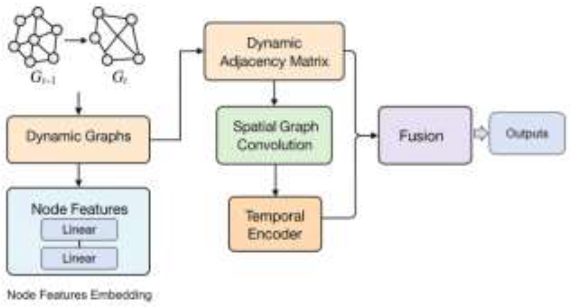
Figure 2.
Sensitivity experiment of the number of graph convolution layers to the model’s MAPE.
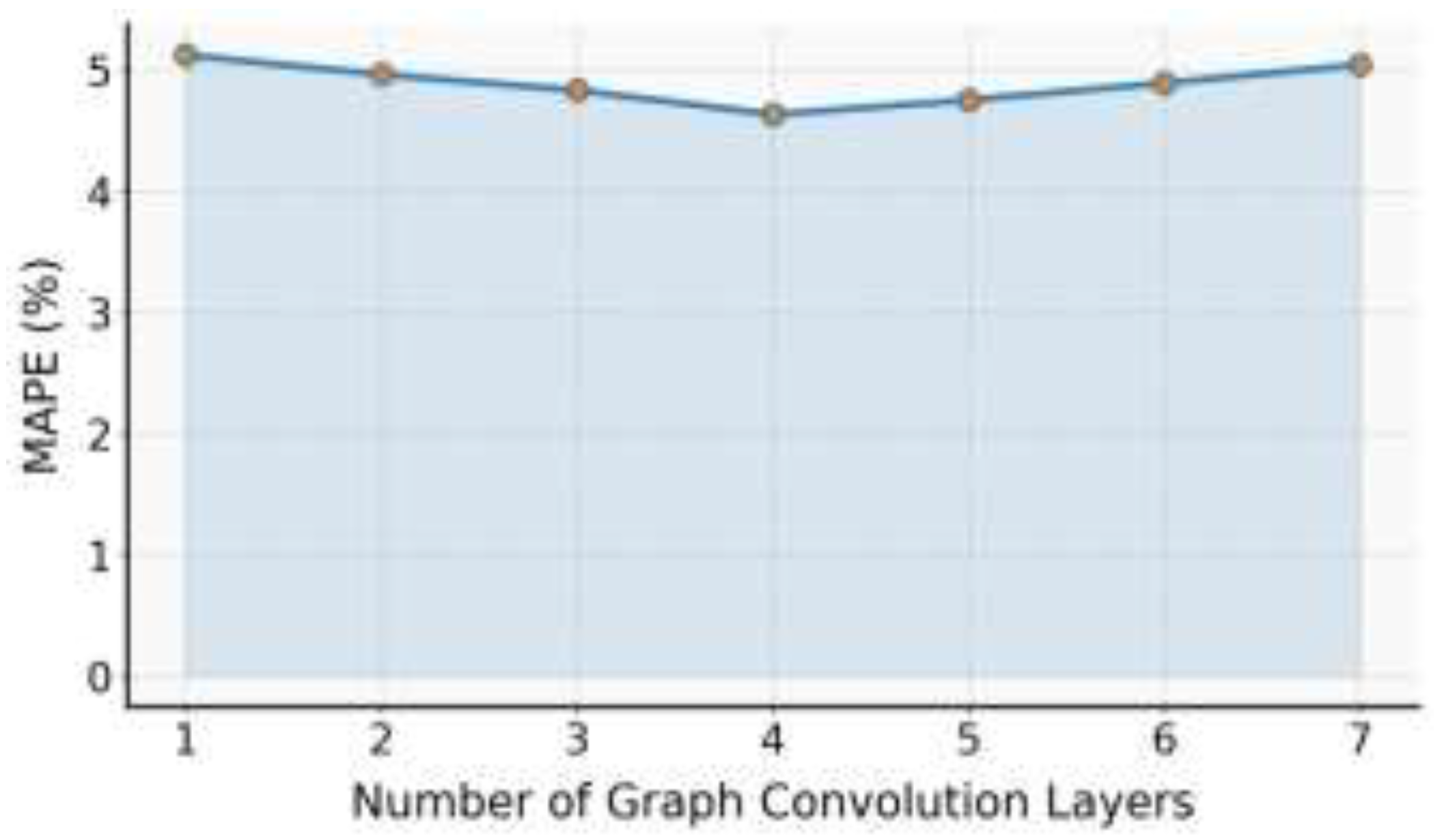
Figure 3.
The impact of the number of attention heads on model experimental results.
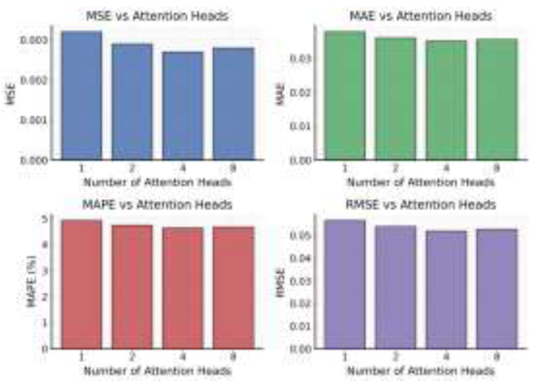
Figure 4.
Sensitivity experiment of adjacency matrix sparsity to model MSE.

Figure 5.
The impact of the number of nodes on the model experiment results.
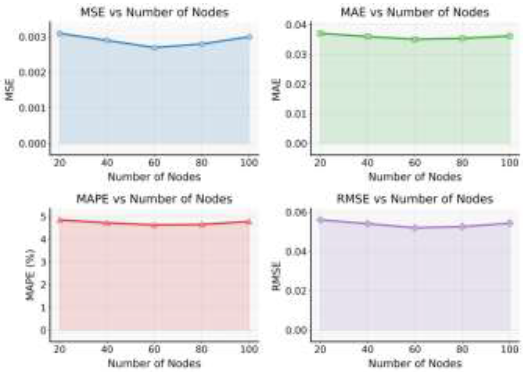

Table 1.
Comparative experimental results.
| Method | MSE | MAE | MAPE | RMSE |
|---|---|---|---|---|
| LSTM[8] | 0.0048 | 0.0482 | 6.37 | 0.0693 |
| BILSTM[9] | 0.0042 | 0.0456 | 6.01 | 0.0648 |
| MLP[10] | 0.0055 | 0.0527 | 7.12 | 0.0741 |
| Transformer[11] | 0.0039 | 0.0433 | 5.68 | 0.0624 |
| BERT[12] | 0.0036 | 0.0418 | 5.44 | 0.0600 |
| Informer[13] | 0.0034 | 0.0395 | 5.19 | 0.0583 |
| Ours | 0.0027 | 0.0351 | 4.63 | 0.0520 |
Disclaimer/Publisher’s Note: The statements, opinions and data contained in all publications are solely those of the individual author(s) and contributor(s) and not of MDPI and/or the editor(s). MDPI and/or the editor(s) disclaim responsibility for any injury to people or property resulting from any ideas, methods, instructions or products referred to in the content. |
© 2026 by the authors. Licensee MDPI, Basel, Switzerland. This article is an open access article distributed under the terms and conditions of the Creative Commons Attribution (CC BY) license (http://creativecommons.org/licenses/by/4.0/).
Copyright: This open access article is published under a Creative Commons CC BY 4.0 license, which permit the free download, distribution, and reuse, provided that the author and preprint are cited in any reuse.


