
Submitted:
02 July 2025
Posted:
04 July 2025
You are already at the latest version
Abstract
Proactive resource allocation is critical for ensuring high availability and efficiency in dynamic, heterogeneous cloud-edge environments. This paper presents a practical and extensible framework for workload prediction and autoscaling, with a focus on virtual Content Delivery Networks (vCDNs). We rigorously evaluate a diverse set of forecasting models, including statistical (Seasonal ARIMA), deep learning (LSTM, Bi-LSTM), and online learning (OS-ELM), using extensive real-world workload traces from a production CDN. Each model is assessed in terms of prediction accuracy, computational cost, and responsiveness to support short-term autoscaling decisions. Predicted workloads are fed into a queue-based resource estimation model to drive proactive provisioning of CDN cache servers. Experimental results show that LSTM-based models consistently deliver the highest accuracy, while lightweight methods such as S-ARIMA and OS-ELM offer efficient, low-overhead alternatives suitable for real-time adaptation or fallback. We further explore adaptive model selection strategies and trade-offs between accuracy, cost, and reactivity. The proposed framework enables accurate, low-rejection autoscaling with minimal overhead and is broadly applicable to other cloud-edge services with predictable workload dynamics.
Keywords:
workload modeling
; workload prediction
; resource allocation
; prediction framework
; ARIMA
; LSTM
; OS-ELM
; CDN
1. Introduction
Large-scale applications deployed across distributed cloud-edge infrastructures, hereafter referred to as cloud-edge applications, must dynamically adapt to fluctuating resource demands in order to maintain high availability and reliability. Such adaptability is typically achieved through elasticity, wherein the system automatically adjusts its resource allocation based on workload intensity. Operationally, elasticity is commonly realized via auto-scaling mechanisms that enable application components to autonomously scale either vertically (adjusting resource capacity of individual instances) or horizontally (modifying the number of component instances), thereby ensuring efficient and resilient service provisioning. Traditional auto-scaling approaches (e.g., those provided by default in commercial platforms such as Amazon AWS1 and Google Cloud2) are reactive, adjusting resources only after performance thresholds are breached. In contrast, proactive auto-scaling aims to anticipate future workload changes and preemptively allocate resources accordingly. This predictive capability hinges on accurate workload forecasting, typically enabled by machine learning or statistical models trained to capture patterns in resource demand [1,2,3] – a task that is inherently challenging, as it requires not only sophisticated forecasting techniques but also a deep understanding of workload dynamics and their temporal evolution.
Workloads in cloud-edge applications are predominantly driven by external request patterns and are often geographically distributed to satisfy localized demand. To effectively model such workloads, key performance indicators, such as “the number of client requests to an application” [3] or the corresponding volume of generated network traffic, are commonly employed. These workload traces are typically captured as time series [4], enabling temporal analysis and forecasting. Classical statistical models, particularly AutoRegressive Integrated Moving Average (ARIMA) and its variants, Seasonal ARIMA (S-ARIMA)[5] and elastic ARIMA[6], have been widely used for this purpose. These methods have demonstrated reasonable predictive accuracy at low computational cost across a variety of workload types [6,7,8]. In addition, modern machine learning (ML) techniques, particularly Recurrent Neural Networks (RNNs), have been extensively applied to workload modeling and prediction due to their ability to capture complex, non-linear temporal patterns. These models offer improved accuracy over traditional approaches for both short- and long-term forecasting [9,10], making them well-suited for dynamic and bursty workload scenarios.
However, in distributed systems such as cloud-edge environments, operational data streams are inherently non-stationary, i.e., they exhibit temporal dynamics and evolve over time due to both external factors (e.g., changes in user behavior, geographical load variations) and internal events (e.g., software updates, infrastructure reconfiguration) [11,12,13]. This evolution often results in a mismatch between the data used to train prediction models and the data encountered during inference, a phenomenon commonly known as concept drift [14]. As a consequence, the accuracy of predictive models deteriorates over time, necessitating regular retraining. Both ARIMA and RNN-based models rely on access to up-to-date historical data for training and updates. While effective, maintaining these models across large scale distributed systems, where millions of data points are processed per time unit, poses significant challenges in terms of scalability, timeliness. To address these issues, online learning techniques have emerged and been integrated into various modeling algorithms, such as Online Sequential Extreme Learning Machine (OS-ELM) [15], Online ARIMA [16], and LSTM-based online learning methods [17]. These approaches enable models to incrementally adapt to streaming data using relatively small updates, making them well-suited for dynamic environments where workloads and system conditions evolve over time. Among these techniques, OS-ELM has gained attention due to its ability to combine the benefits of neural networks and online learning while maintaining low computational complexity, which enhances its practicality in large-scale cloud-edge systems.
Building on this foundation, we present a framework for constructing predictive workload models designed to support proactive resource management in large-scale cloud-edge environments. The framework is validated through a practical use case involving CDNs, a class of applications characterized by highly variable and large-scale traffic patterns. To accommodate the multi-timescale nature of CDN workloads, we systematically investigate both offline and online learning methods. The evaluation spans a range of modeling techniques, including statistical forecasting, Long Short-Term Memory (LSTM) networks, and OS-ELM, all trained on operational CDN datasets. Further, these models are integrated into a unified prediction framework intended to provide workload forecasting capabilities to autoscalers and infrastructure optimization systems, enabling proactive and data-driven scaling decisions. We conduct a thorough performance evaluation based on prediction accuracy, training overhead, and inference time, in order to assess the applicability and efficiency of each approach within the context of the CDN use case. Ultimately, the goal of this work is to develop a robust and extensible framework for transforming workload forecasts into actionable resource demand estimates, leveraging system profiling, machine learning, and queuing theory.
The main contributions of this work are as follows:
- (i)
- A comprehensive workload characterization and pattern based on operational trace data collected from a large-scale real-world CDN system.
- (ii)
- The development of a predictive modeling pipeline that combines statistical and machine learning methods, both offline and online, to capture workload dynamics across different time scales.
- (iii)
- A unified framework that links workload prediction with resource estimation, enabling proactive auto-scaling in cloud-edge environments.
- (iv)
- Empirical validation of the framework on real-world CDN traces, measuring prediction fidelity, computational efficiency, and runtime adaptability.
The remainder of the paper is organized as follows: Section 2 surveys related work; Section 3 introduces the targeted application, i.e., the BT CDN system3, its workload, and workload modeling techniques utilized in our work; Section 4 introduces datasets, outlines workflows and methodologies, and presents the produced workload models along with an analysis of results; Section 5 presents a framework composed of the produced workload models and a workload to resource requirements calculation model; Section 6 discusses future research directions; and Section 7 concludes the paper.
2. Related Work
Understanding system performance, application behavior, and workload characteristics is fundamental to enabling elasticity and proactive resource allocation. Consequently, these topics have received extensive attention in the literature over the past decade, as reviewed in several comprehensive surveys [3,18,19]. This section discusses related work with a particular emphasis on workload modeling and prediction techniques, as well as auto-scaling mechanisms.
2.1. Workload Modeling and Prediction
Workload modeling and prediction in large-scale distributed applications and datacenters’ infrastructure has been addressed earlier using classical statistical models such as auto-regression, Markov models, and Bayesian models [7,20,21]. Rossi et al. [20,21] propose a Hybrid Bayesian Neural Network (HBNN) that integrates a Bayesian layer into an LSTM architecture to model both epistemic and aleatoric uncertainty in CPU and memory workload prediction. Using variational inference, the model outputs a Gaussian distribution over future demand, enabling computation of confidence-based upper bounds for proactive resource allocation. Experiments on Google Cloud trace data show that HBNN achieves comparable point prediction accuracy to standard LSTM while reducing overprovisioning and total predicted resources for the same QoS targets. Also targeting proactive workload prediction, the work in [22] first clusters virtual machines (VMs) into different groups exhibiting particular workload patterns. The authors next build a Hidden Markov model-based method leveraging the temporal correlations in workloads of each group to predict the workload of each individual VM. The method is claimed to possibly improve the prediction accuracy up to 76% compared to traditional methods using only individual server level (i.e., single time series based methods). Sheng et al.propose a Bayesian method in [23] to predict the average resource utilization in terms of CPU and memory for both long-term intervals (e.g., up to 16 hours) and consecutive short-term intervals (e.g., every 2 minutes). Through experiments with Google’s data traces, the proposed method is shown to achieve a high accuracy regardless of the degree of workload fluctuation and to outperform existing auto-regression and filter-based methods. With the same targeted domain as the focus in this present work, we employ S-ARIMA to model the workload of a CDN cache server [7]. The obtained predictive model basically meets our main requirement of workload predictions for the targeted CDN. Moreover, the preliminary results including the workload analysis, the statistical workload model and the application model present in the work lay a foundation for our extension in this present study.
Apart from classical statistical methods, ML techniques have recently been widely adopted for workload prediction in the highly distributed computing platforms [24,25,26]. Kumar et al.propose an online workload prediction model based on the ELM technique [24]. The model adopts the rapid yet high accurate learning process of ELM to forecast the workload arrival in very short time intervals. Extensive experiments using Google workload traces show that the proposed ELM outperforms the state-of-the-art techniques, including ARIMA, Support Vector Regression (SVR), by surprisingly reducing the mean prediction error from 11% up to 100%. Another online resource utilization predictive model using spare Bidirectional LSTM (Bi-LSTM) is proposed in [25]. The authors improve the learning time of a classical Bi-LSTM by constructing a fewer-parameter Bi-LSTM model that is more efficient for online prediction. The model is evaluated through experiments with Google and PlanetLab data, and the results show that besides a high prediction accuracy, the model’s training time is reduced by 50% – 60% compared to the classical Bi-LSTM model. The aforementioned techniques rely on the analysis of just a single server or application workload, which are probably working inefficiently in the context of highly distributed cloud-edge platforms. With a consideration of the user mobility behavior in such cloud-edge computing environments, Nguyen et al.propose a location-aware workload prediction model for edge datacenters (EDCs) [26]. The proposed multivariate-LSTM-based model exploits the correlation in workload changes among EDCs within close proximity to each other so as to forecast the future workload for each of them. It is finally proven, through experiments, to achieve a robust performance with considerably improved prediction accuracy compared with other recent advanced methods.
2.2. Elasticity in Large-Scale Cloud-Edge Systems
Aiming at reliable, cost- and energy-efficient computing platforms, diverse techniques and methodologies have been devised to implement elasticity or auto-scaling (sub)systems. Existing implementations rely on either a rule-based or a model-based approach in tackling the elasticity in a reactive or proactive manner. While the rule-based approach has been more popular and widely adopted in many commercial products thanks to its straightforward deployment and high reliability, the proactive one, backed by aforementioned modeling and prediction techniques, is shown to be more complicated and advanced, hence drawing more attention from the research community.
By adopting the rule-based elasticity, commercial cloud-based resource providers simply offer a user interface enabling clients to define performance metric thresholds of, e.g., resource utilization, rejection rates, or service response times, and corresponding scaling plans to be executed. Based on these settings, resources are then automatically allocated for the applications in order to reactively adapt to their performance changes. Examples for this approach include Kubernetes [27] and Amazon AWS [28] which rely on their own rule-based autoscalers to perform applications’ horizontal auto-scaling.
A recent work proposing a hybrid proactive auto-scaling mechanism, namely Chameleon, has been presented in [29]. Its auto-scaling framework incorporates multiple proactive methods coupled with a reactive mechanism to facilitate the resource allocation. The framework adopts time series analysis to forecast the arriving load intensity and relies on queuing theory to estimate resource demands. The authors of the work next propose Chamulteon, an enhanced version of Chameleon, enabling the coordinated scaling of microservice applications [30]. The Chamulteon auto-scaling framework is implemented with two sub-functions: a reactive one to perform scaling tasks for the microservices respecting the resource demand in short time intervals, and a proactive one relying on workload prediction to proactively perform such tasks in longer time intervals. The framework is shown to outperform notable autoscalers through experiments using real world data traces, and conducted in various environments with different virtualization technologies.
In a related effort, Bhardwaj et al. [31] introduces a performance-aware resource allocator that learns resource-to-performance mappings online and incorporates uncertainty through ARMA-based load forecasting with 90% confidence bounds. Its modular design supports both multi-tenant and microservice workloads and demonstrates improved utility and tail latency compared to existing baselines. Building on the theme of SLO-driven autoscaling, Jeon et al. [32] proposes a system tailored for fixed-size on-premises ML inference clusters, allowing developers to specify latency SLOs directly. Faro dynamically autoscale inference job replicas to maximize cluster-wide utility, integrating with Ray Serve on Kubernetes, and achieves significantly fewer SLO violations, i.e, 2.3× to 23× improvement over prior methods under real-world workloads. Complementing these works, Liu et al. [33] addresses elasticity challenges in serverless platforms by decoupling prediction from scheduling to reduce overhead and employing dual-staged scaling to enable fast, low-cost resource adjustments. This design improves deployment density and resource utilization while significantly reducing cold start latency and scheduling costs compared to state-of-the-art schedulers. In another extreme, Nguyen et al. [34] present a location-aware proactive elastic controller for dynamic resource provisioning targeting latency-intolerant mobile edge applications. Their controller comprises four components: a multivariate LSTM-based location-aware workload predictor capturing correlations across adjacent edge data centers (EDCs); a queuing-theory-based performance modeler; a group-based resource provisioner for scaling resources at each EDC; and a weighted round-robin load balancer for real-time user request distribution. Extensive experiments with real user-mobility data demonstrate significant improvements in scaling capability and resource provisioning efficiency over state-of-the-art reactive controllers.
3. CDN Systems and Workloads
This section examines workload modeling and prediction for large-scale distributed cloud-edge applications, with CDNs serving as a real-world case study. We analyze the architecture and operational workload characteristics of a production-scale multi-tier CDN system operating globally, identifying key spatiotemporal patterns. Based on these insights, we then explore both time series statistical modeling approaches, specifically S-ARIMA, and ML techniques – including LSTM-based RNNs and OS-ELM – as candidates for robust predictive models.
3.1. A Large-Scale Distributed Application and Its Workload
CDNs efficiently distribute internet content using large networks of cache servers (or caches), strategically placed at network edges near consumers. This content replication benefits all stakeholders, i.e., consumers, content providers, and infrastructure operators, by improving Quality of Experience (QoE) and reducing core network bandwidth consumption. Modern CDNs are increasingly architected as virtualized infrastructures, deploying software-resolved caches (vCaches) in containers or VMs across cloud-edge resources. This virtualization facilitates the flexible and rapid deployment of multi-tier caching networks for large-scale virtual CDNs (vCDNs) [7]. Leveraging the hierarchical nature of networks, this multi-tier model significantly enhances CDN performance [35,36,37]. For instance, Figure 1 illustrates a conceptual model of BT’s production vCDN system, where vCaches are deployed across hierarchical network tiers (T1, Metro, Core).
To provide a concrete basis for our analysis, this paper investigates the BT CDN and its operational workloads. This CDN employs a hierarchical caching structure where each cache possesses at least one parent cache in a higher network tier, culminating in origin servers as the ultimate source of content objects. Content delivery adheres to a read-through caching model, i.e, a cache miss triggers a request forwarding to successive upper vCaches until a hit is achieved or the highest tier vCache is reached. Should no cache hit occur within the CDN, content objects are retrieved from their respective origin servers and are subject to local caching for subsequent demands.
Workload datasets collected from the BT CDN are analyzed and modeled for prediction, as detailed in Section 4. Consistent with the read-through model, workload at core network vCaches is significantly higher than at edge vCaches, a characteristic evident in our exploratory data analysis and visually represented in Figure 2. Furthermore, our analysis reveals a distinct daily seasonality in the workload data: minimum traffic volumes are recorded between 01:00 and 06:00, while peak traffic occurs from 19:00 to 21:00. This pattern aligns with typical user content access behaviors and reinforces conclusions from our prior investigation into BT CDN workload characteristics [7].
3.2. Statistical Workload Modeling
For time series analysis, especially with seasonal data, S-ARIMA is a well-established and computationally efficient method for constructing predictive models [5,7]. Given the pronounced daily seasonality identified in the BT CDN workload datasets, we employ S-ARIMA to generate short-term workload predictions.
As described in [5], an S-ARIMA model comprises three main components: a non-seasonal part, a seasonal part, and a seasonal period (S) representing the length of the seasonal cycle in the time series. This model is formally denoted as . Here, the hyperparameters specify the orders for the non-seasonal auto-regressive, differencing, and moving-average components, respectively, while denote these orders for the seasonal part. S-ARIMA models are constructed using the Box-Jenkins methodology, which relies on the auto-correlation function (ACF) and partial auto-correlation function (PACF) for hyperparameter identification. Model applicability is then validated using the Ljung-Box test [38] and/or by comparing the time series data against the model’s fitted values. Finally, the Akaike Information Criterion (AIC) or Bayesian Information Criterion (BIC) serves as the primary metric for optimal model selection.
3.3. Machine Learning based Workload Modeling
In contrast to traditional statistical methods, ML techniques derive predictive models by learning directly from data, without requiring predetermined mathematical equations. Given the necessity for solutions that support resource allocation and planning across varying time scales, and that meet stringent requirements for practicality, reliability, and availability, we employ two specific ML candidates for our workload modeling: LSTM-based RNNs and OS-ELM.
3.3.1. LSTM-Based RNN
Artificial Neural Networks (ANNs) are computational models composed of interconnected processing nodes with weighted connections. Based on their connectivity, ANNs broadly categorize into two forms [39]: Feed-forward Neural Networks (FNNs), which feature unidirectional signal propagation from input to output, and Recurrent Neural Networks (RNNs), characterized by cyclical connections. The inherent feedback loops in RNNs enable them to maintain an internal “memory" of past inputs, significantly influencing subsequent outputs. This temporal persistence provides RNNs with distinct advantages over FNNs for sequential data. In this work, we adopt two prominent RNN architectures, LSTM and Bidirectional LSTM (Bi-LSTM), widely recognized for their efficacy in capturing temporal dependencies within time series data.
- LSTM: With the overall rapid learning process and the efficiency in handling the vanishing gradient problem, LSTM has been preferred and achieved record results in numerous complicated tasks, e.g., speech recognition, image caption, and time series modeling and prediction. In essence, an LSTM includes a set of recurrently connected subnets; each contains one or more self-connected memory cells, and three operation gates. The input, output and forget gates respectively play the roles of write, read and reset operations for memory cells [40]. An LSTM RNN performs its learning process in a multi-iteration manner. For each iteration, namely epoch, given an input data vector of length T, the vectors of gate units and memory cells, with the same length, are updated through a two-step process including the forward pass recursively updating elements of each vector one by one from the 1st to the element, and the backward pass carrying out the update recursively in reverse direction.
- Bi-LSTM: It is an extension of the traditional LSTM in which for each training epoch, two independent LSTMs are trained [41]. During training, a Bi-LSTM effectively consists of two independent LSTM layers: one processes the input sequence in its original order (forward pass), while the other processes a reversed copy of the input sequence (backward pass). This dual processing enables the network to capture contextual information from both preceding and succeeding elements in the time series, leading to a more comprehensive understanding of its characteristics. Consequently, Bi-LSTMs often achieve enhanced learning efficiency and superior predictive performance compared to unidirectional LSTMs.
3.3.2. OS-ELM
OS-ELM is distinguished as an efficient online technique for time series modeling and prediction. It delivers high-speed forecast generation, often achieving superior performance and accuracy compared to certain batch-training methods in various applications. OS-ELM’s online learning paradigm allows for remarkable data input flexibility, processing telemetry as single entries or in chunks of varying sizes.
Unlike conventional iterative learning algorithms, OS-ELM’s core principle involves randomly initializing input weights and then rapidly updating output weights via a recursive least squares approach. This strategy enables OS-ELM to adapt swiftly to emergent data patterns, which often translates to enhanced predictive accuracy over other online algorithms [42]. In essence, the OS-ELM learning process includes two fundamental phases:
- (i)
- Initialization: A small chunk of training data is required to initialize the learning process. The input weights and bias for hidden nodes are randomly selected. Next, the core of the OS-ELM model including the hidden layer output matrix and the corresponding output weights are initially estimated using these initial input parametric components.
- (ii)
- Sequential Learning: A continuous learning process is applied to the collected telemetry iteratively. In each iteration, the output matrix and the output weights are updated using a chunk of new observations. The chunk size could be different through iterations. Predictions can be obtained continuously after every sequential learning.
Comprehensive details regarding OS-ELM implementation, including calculations and procedures, are available in [15].
4. Workload Modeling and Prediction
This section provides a detailed account of our approach to workload modeling and prediction for large-scale distributed cloud-edge applications. We begin by describing the real-world dataset collected from a core BT CDN cache, which serves as the empirical foundation for our analysis. Subsequently, we outline the comprehensive workflow guiding our data processing, model construction, and prediction phases. We then establish our methodology, detailing crucial steps from data resampling and training dataset selection to multi-criteria continuous modeling and rigorous model validation. Finally, we present and discuss the experimental results, including performance evaluations across various models and metrics.
4.1. Dataset
The experimental foundation of this work relies on a workload dataset collected from multiple cache servers of the BT CDN [43]. This dataset spans 18 consecutive months between 2018 and 2019, providing time series data with a one-minute interval. Each data point represents the workload, specifically traffic in bits per second (bps), served by the cache servers.
For our experiments, we specifically utilize the dataset collected at a single cache in the core BT network layer, where the highest degree of workload is consistently observed.
4.2. Workflow
The comprehensive workflow for our workload modeling and prediction process is illustrated in Figure 3.
The process begins with the workload collector, which instruments production system servers and infrastructure networks across multiple locations to gather metric and Key Performance Indicator (KPI) measurements as time series data. Subsequently, an exploratory data analysis (EDA) is regularly performed offline on the collected data to gain insights into workload and application behaviors, identify characteristics, and reveal any data anomalies for cleansing.
Knowledge derived from the EDA is then fed to a workload characterizer, responsible for extracting key workload features and characteristics. This extracted information directly informs the parameter settings for modeling algorithms within the workload modelers. Multiple workload modelers, employing various algorithms, train and tune models to capture the governing dynamics of the workloads, storing these models for identified states in model descriptions.
Finally, a workload predictor utilizes these model descriptions, incorporating semantic knowledge of desired application behavior, to interpret and forecast future states of monitored system workloads. Workload predictors are typically application-specific, request-driven, and serve as components in application autoscalers or other infrastructure optimization systems.
Further details about the workflow pipeline, including the mapping of the conceptual services to architecture components as well as a concrete example of usage of the framework is available in Section 5.1.
4.3. Methodology
To effectively accomplish workload modeling and prediction for the BT CDN, it is firstly required an initial analysis of the application structure together with an EDA on its telemetry as described in Section 3.1. Such analysis is crucial for establishing a robust methodology. Accordingly, this section details the key procedures of our designated methodology.
4.3.1. Resampled Datasets
To support near real-time horizontal auto-scaling with short-term workload predictions, we target a 10-minute prediction interval. While earlier studies reported high variability in VM startup times across platforms [44], recent advances in virtualization and orchestration technologies have significantly reduced these delays, often bringing VM and container initialization into the sub-minute range [45,46,47].
Nevertheless, in practical large-scale systems such as our virtualized CDN deployment, end-to-end readiness encompasses more than just infrastructure spin-up, i.e., it also includes application warm-up, cache synchronization, and routing stabilization, which may still require several minutes before the instance becomes fully effective. Furthermore, our empirical analysis of the CDN workload reveals limited fluctuation at sub-hour granularity, with clear and recurring daily cycles (see Figure 2). Given these observations, we evaluate prediction models using two resampling intervals: 10 minutes and 1 hour. These datasets, referred to as the original datasets, enable us to study the trade-offs between prediction granularity, system responsiveness, and modeling efficiency.
4.3.2. Appropriate Size of Training Datasets
Our analytical results on the original datasets demonstrate that using appropriately sized data chunks for training yields models with superior workload pattern capturing and predictability, compared to training on entire original datasets. This observation is consistently aligned with both our previous work [7] and other relevant studies [13,48].
Consequently, we divide each original dataset into multiple data chunks, constructing distinct models for each using our selected techniques. We systematically tested various chunk sizes and selected the one yielding the most accurate predictions on average. For a fair comparison across all adopted modeling techniques, we employed a single, universally applicable chunk size for model construction, validation, and evaluation in this work. Specifically, we chose chunk sizes of two months for the 10-minute dataset and four months for the 1-hour dataset. These processed segments are hereafter referred to as data chunks (e.g., 10-minute data chunk, 1-hour data chunk), serving as our training datasets for workload modeling.
4.3.3. Multi-Criteria Continuous Workload Modeling
As detailed in Section 3, our work employs multiple modeling techniques to construct predictive workload models, leveraging their distinct advantages. We apply S-ARIMA and OS-ELM to both 10-minute and 1-hour training datasets. LSTM is applied exclusively to the 1-hour dataset, while Bi-LSTM is used for the 10-minute dataset.
Each technique serves a specific role: S-ARIMA offers a lower training cost with an expectation of reasonable accuracy compared to LSTM-based methods. LSTM-based techniques are anticipated to yield the highest predictive accuracy. OS-ELM, conversely, is the fastest in both training and prediction, making it the preferred candidate for near real-time auto-scaling or as a fallback when other models are unavailable. Bi-LSTM is specifically chosen for the 10-minute dataset due to its ability to efficiently capture patterns without explicit seasonality, outperforming standard LSTM in such contexts.
Models built using 1-hour and 10-minute training datasets are subsequently referred to as 1-hour models and 10-minute models, respectively (e.g., 1-hour S-ARIMA models, 10-minute OS-ELM models).
For real-world scenarios, our approach emphasizes a continuous modeling and prediction process where models are frequently updated with newly collected data to maintain accuracy over time. To achieve this, we employ a sliding window mechanism to segment the original datasets into training chunks. Given that our chosen chunk sizes are two months for the 10-minute dataset and four months for the 1-hour dataset (as presented in Section 4.3.2), we set a one-month step for this sliding window to extract these data chunks. This means models are utilized for predictions for a maximum of one month before being updated with fresh data, reflecting a practical cycle for continuous model refinement. While actual deployments might require more frequent updates (e.g., weekly or daily), our chosen step provides a robust evaluation framework. Ultimately, for each selected modeling technique, a distinct set of models is constructed, with one model corresponding to each data chunk derived from the entire original datasets.
4.3.4. Model Validation
The predictability of the constructed models is validated using the rolling forecast technique which produces one-step predictions iteratively. For each ML model, a series of real data values, corresponding to a number time-steps, is given to retrieve the next time-step prediction in each iteration. Different from that, a S-ARIMA model produces a next time-step prediction itself and then is tuned with the real data value observed at that time-step so as to be ready for the forthcoming predictions.
To illustrate the model validation, we perform predictions, precisely out-of-sample predictions, continuously for every 10 minutes in one day and every one hour in one week using each of the 10-minute models and the 1-hour models, respectively. In other words, we collect workload predictions for 144 consecutive 10-minute time periods and 148 consecutive 1-hour periods for each of the corresponding models. Next, the set of predictions obtained by each model is compared to a test dataset of real workload observations extracted from the corresponding original dataset at the relevant time period of the predictions. This means in order to facilitate such a comparison for each case of model construction, after retrieving a training dataset, a test dataset containing a number of consecutive data points at the same periods is also reserved.
Because every ML model requires an input data series to produce a prediction, in order to accomplish the model validation, we form a validation dataset by appending the test dataset to the input series of the last epoch of the training process. Next, a sliding window of size m is defined on the validation dataset to extract a piece of input data for every prediction retrieval from the model, where m denotes the size or the number of samples of the input series for each training epoch, which is generally called the size of the input of an ML model. The structure of such a validation dataset together with a sliding window defined on it is illustrated in Figure 4.
In case of S-ARIMA, our implementation requires a model update after each prediction retrieval, thus we keep updating the model with observations in the test dataset one by one during the model validation process.
4.4. Experimental Results
With the selected chunk sizes of two months and four months (see Section 4.3.2), we obtain two sets of 16 10-minute and 14 1-hour data chunks from the corresponding 10-minute and 1-hour original datasets. For every single data chunk, three modeling techniques are applied to generate different models.
- S-ARIMA: The 1-hour S-ARIMA models are constructed with a seasonality so as to capture the daily traffic pattern. This value of seasonality is also applied to 10-minute models, which implies a consideration of 4-hour traffic patterns, because no explicit seasonality is observed within hours from 10-minute data chunks through our EDA. The rest of hyperparameters are identified using the method presented in Section 3.2.
- LSTM-based: Because quite simple patterns exist in every entire 1-hour and 10-minute dataset, we use only one single hidden layer for both LSTM and Bi-LSTM algorithms with 24 and 32 neurons, respectively. The number of input neurons is fixed at 40 for both algorithms. Learning rates are also fixed during the training process of the two algorithms. Experiments show that Bi-LSTM converges faster at 150 epochs than LSTM at 270 epochs.
- OS-ELM: We also apply one single hidden layer to the training algorithm for all cases. Due to the strong seasonality in the workload, 1-hour OS-ELM models are constructed simply with 48 input neurons and 35 hidden neurons for all cases, while these hyperparameters of 10-minute OS-ELM models are varied case by case.
In order to confirm the variants of resulting models due to the random initialization in ML techniques as well as to establish a confidence in the collected models, we execute 10 runs on each combination of a technique and a data chunk, i.e., 10 variants of model are collected for each combination, and then utilize all these variants to perform predictions. Note that all the runs are executed in servers with the same configuration and without GPU support, which are deployed in a computer cluster. The accuracy of every model is assessed based on the prediction results and illustrated through a typical error metric, namely the symmetric mean absolute percentage error (SMAPE) which has been widely used to evaluate the accuracy of regression models [49,50,51] and is given by:
where n denotes the size of the set of data points, and and denote the observation and the prediction at time i, respectively. Apparently, a small value of SMAPE indicates the high accuracy in terms of the predictability of a model.
To summarize, each original dataset yields a corresponding result set comprising the trained models, their predictions, prediction errors, and associated training and inference times. Accordingly, we derive two result sets: one for the 10-minute dataset and another for the 1-hour dataset. Each result set includes multiple models built on different training chunks, and due to space constraints, we highlight only two representative subsets per result set for detailed analysis and comparison.
Specifically, we select two representative model groups: (i) the best-case models, consisting of one top-performing model per technique (S-ARIMA, LSTM-based, and OS-ELM), and (ii) the worst-case models, which exhibit the poorest performance among their respective types. For the 10-minute result set, models built using the 3rd and 10th data chunks, corresponding to [Mar–Apr 2018] and [Oct–Nov 2018], respectively, are shown in Figure 5 and Figure 6. Similarly, for the 1-hour result set, the selected models are the 1st and 9th, illustrated in Figure 9 and Figure 10.
Each figure includes a full view of predictions across the test period (Figure 5a, Figure 6a, Figure 9a and Figure 10a) and a zoomed-in view (Figure 5b, Figure 6b, Figure 9b and Figure 10b) to support more granular comparisons. To further assess model accuracy and robustness, we present a summary of prediction errors across all models in Figure 8 and Figure 12, respectively. Additionally, the mean prediction error across 10 independent runs for each model type is reported in Figure 13.
Figure 5.
Performance of the three 10-minute models in the worst scenario (data chunk of [Mar-2018 – Apr-2018])
Figure 5.
Performance of the three 10-minute models in the worst scenario (data chunk of [Mar-2018 – Apr-2018])
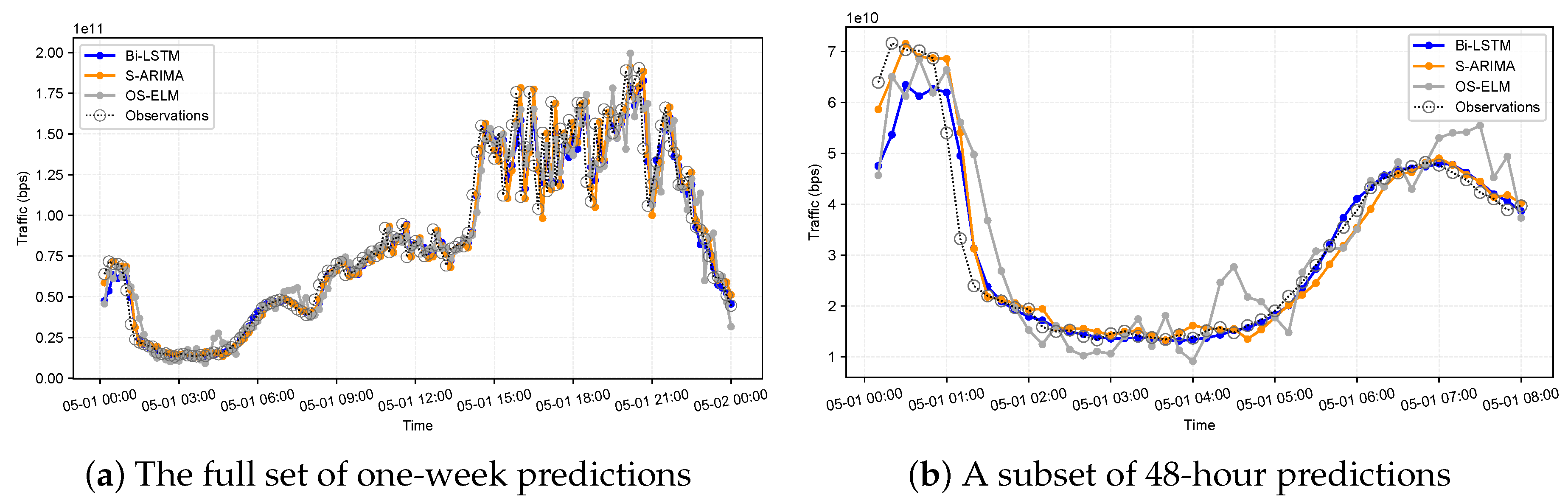
Figure 6.
Performance of the three 10-minute models in the best scenario (data chunk of [Oct-2018 – Nov-2018])
Figure 6.
Performance of the three 10-minute models in the best scenario (data chunk of [Oct-2018 – Nov-2018])
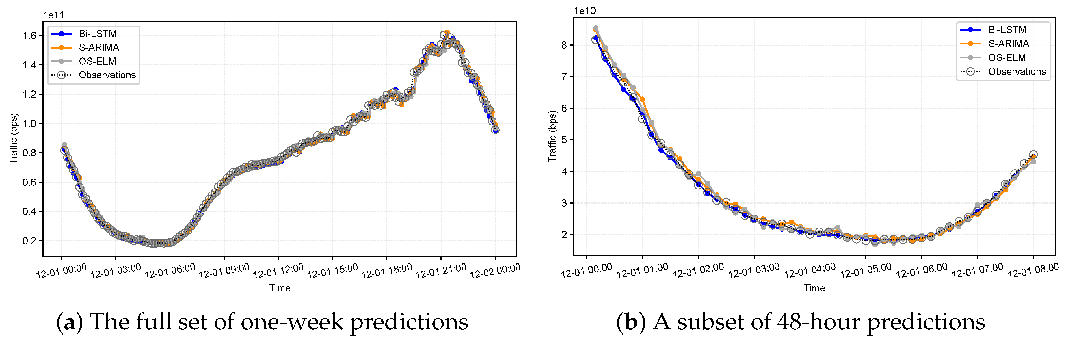
Figure 7.
Average training and prediction time of 10-minute models
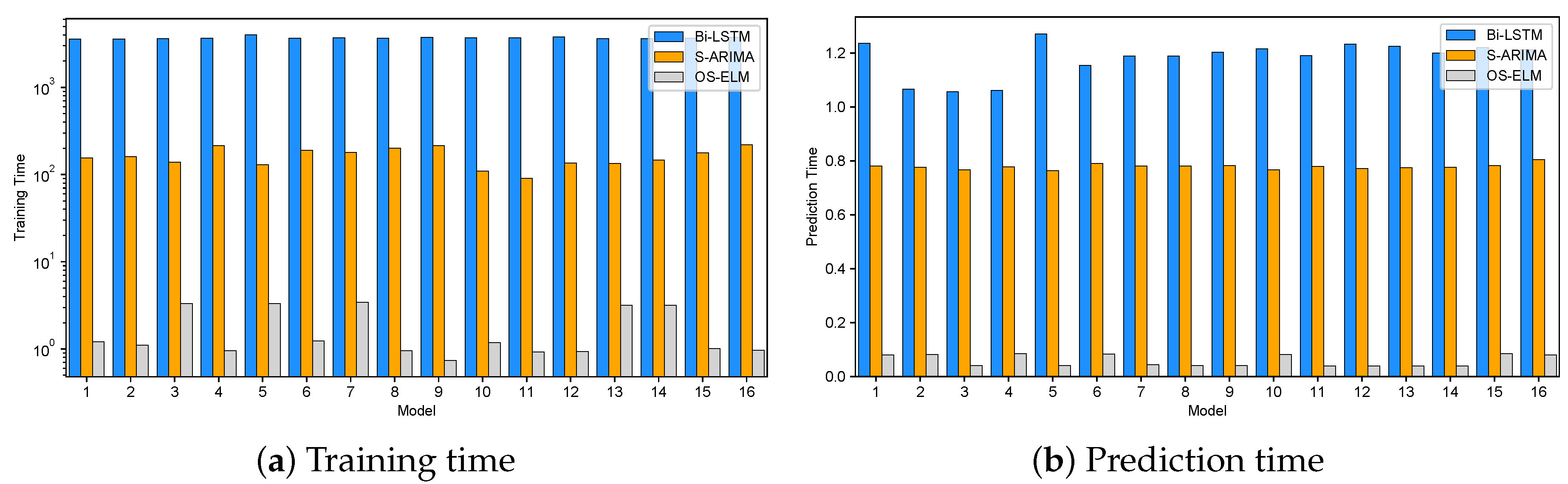
Figure 8.
Prediction errors of 10-minute models.
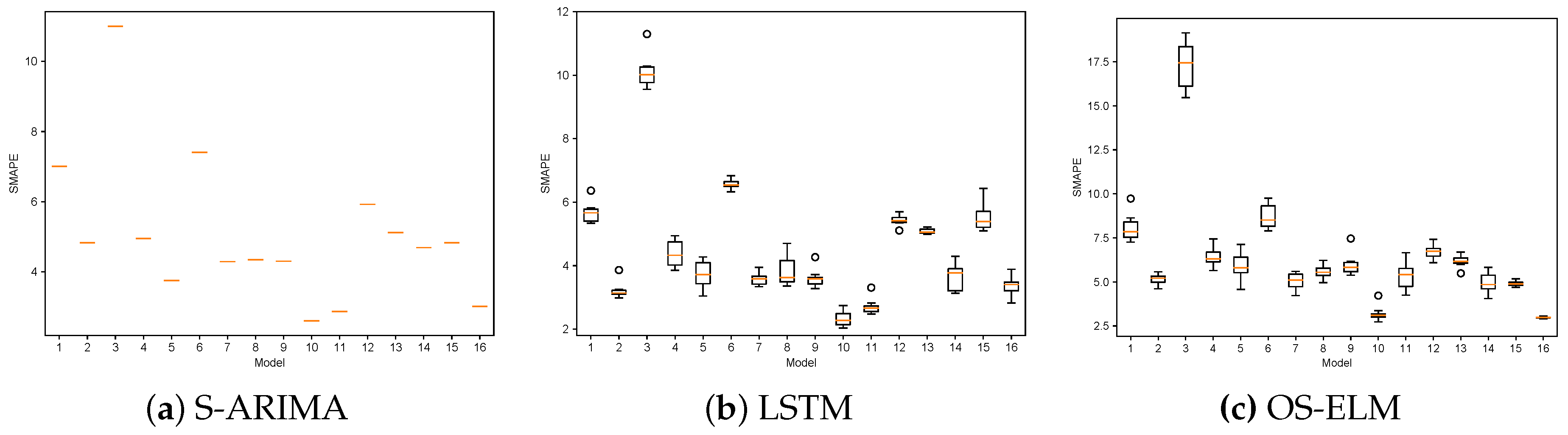
Figure 9.
Performance of the three 1-hour models in the worst scenario (data chunk of [Jan-2018 – Apr-2018])
Figure 9.
Performance of the three 1-hour models in the worst scenario (data chunk of [Jan-2018 – Apr-2018])
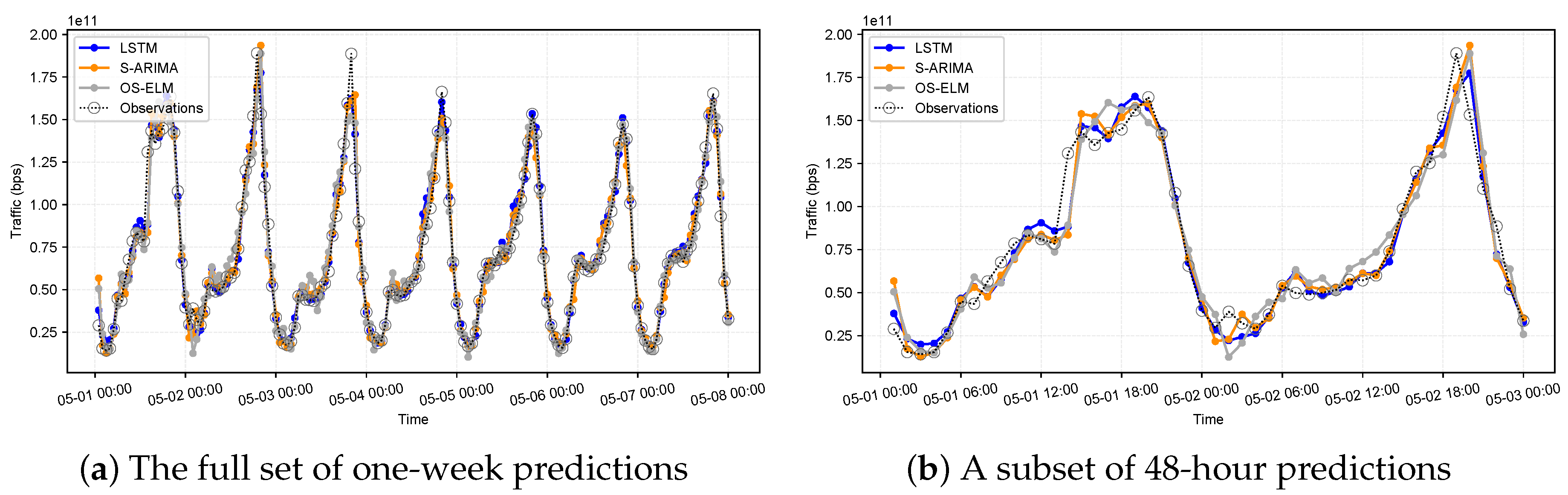
Figure 10.
Performance of the three 1-hour models in the best scenario (data chunk of [Sep-2018 – Dec-2018])
Figure 10.
Performance of the three 1-hour models in the best scenario (data chunk of [Sep-2018 – Dec-2018])
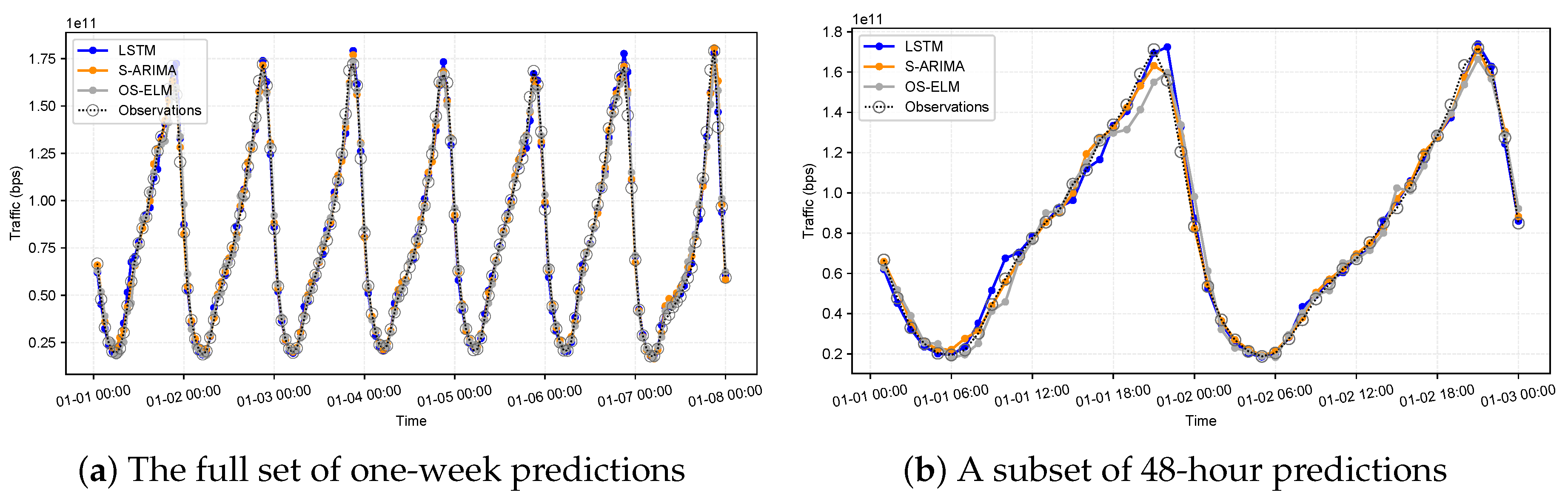
Figure 11.
Average training and prediction time of 1-hour models
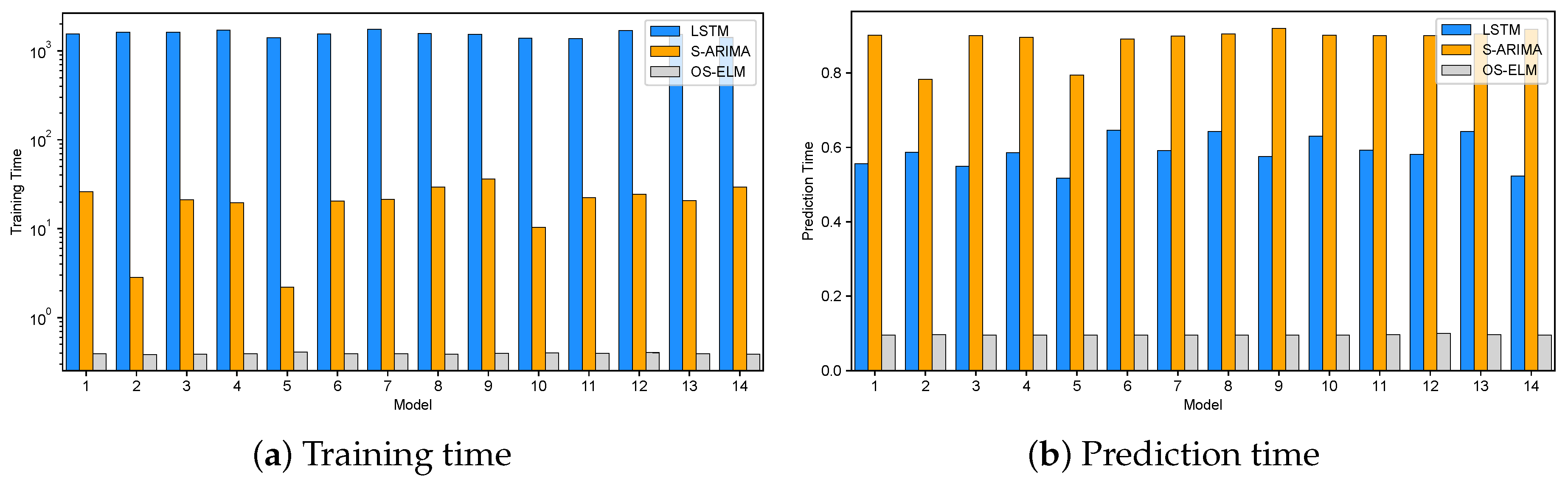
Figure 12.
Prediction errors of 1-hour models
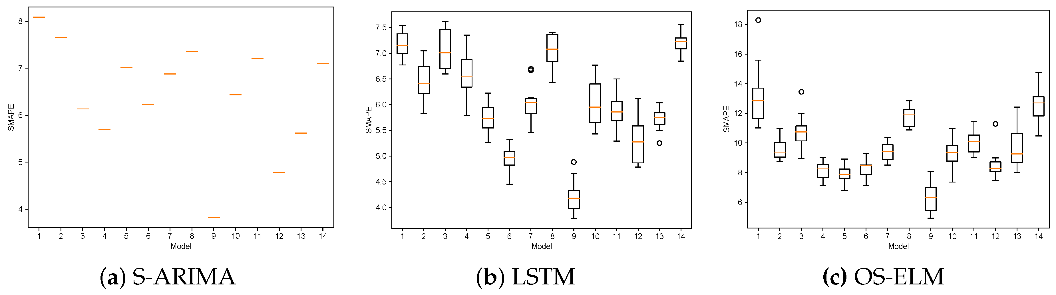
Figure 13.
Average prediction error of the models.
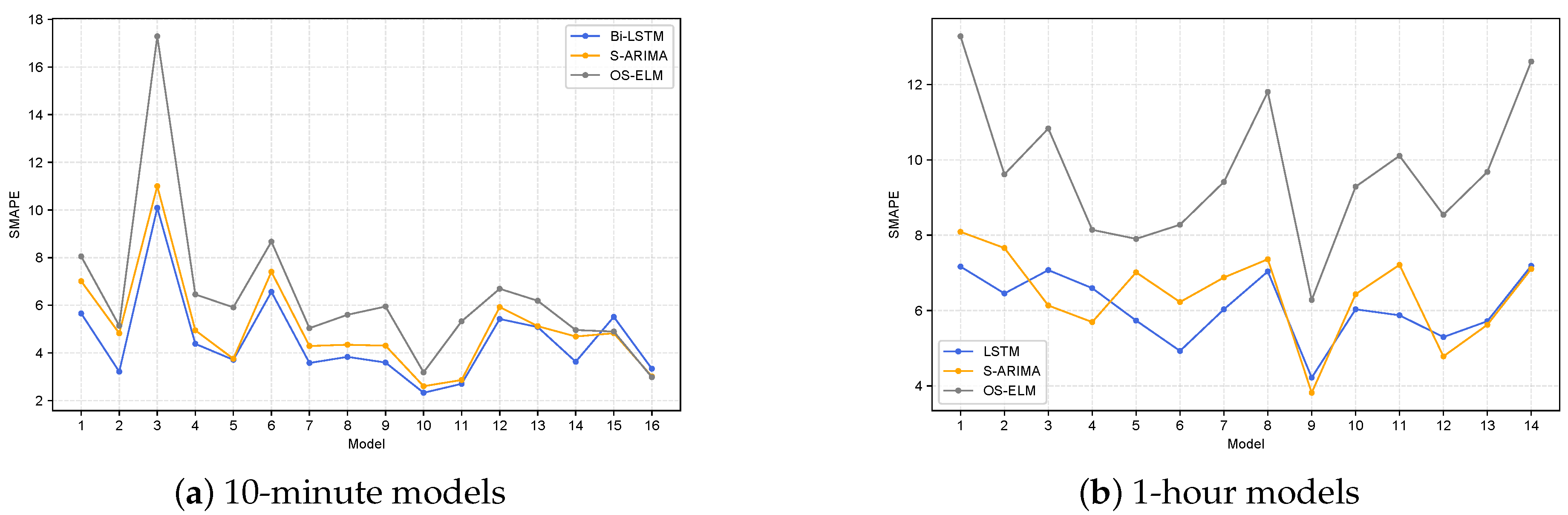
4.4.1. Performance Comparison within Each Modeling Technique
As illustrated in Figure 5, Figure 6, Figure 9, and Figure 10, each dataset exhibits seasonality, yet distinct traffic patterns emerge across different time periods. These variations in workload behavior validate our approach of training models on smaller, time-localized data chunks rather than the full dataset, enabling more accurate short-term predictions. The figures also highlight noticeable performance differences among models of the same type trained on different chunks. For instance, in the case of 10-minute models, those trained on data from Mar–Apr 2018 consistently underperform compared to models trained on Oct–Nov 2018, as seen in Figure 5 and Figure 6. A similar trend is observed for the 1-hour models in Figure 9 and Figure 10. These discrepancies are further quantified through the prediction error metrics shown in Figure 8 and Figure 12.
Takeaway. The observed variability in workload behavior across different time periods, even within the same seasonal cycle, supports the effectiveness of training models on time-localized data chunks. This approach enables the models to better capture short-term dynamics and leads to improved prediction accuracy compared to training on the full dataset.
4.4.2. Cross-Technique Performance Evaluation Across Modeling Methods and Training Data
To enable informed model selection for proactive scaling under diverse operational scenarios, it is essential to compare models constructed using different prediction techniques and training data.
From the comparative illustrations in Figure 8, Figure 12, and Figure 13, it is evident that LSTM-based models consistently outperform other techniques in most cases. Specifically, over 90% of the 10-minute and 1-hour LSTM models exhibit prediction errors below 6% and 7.25%, respectively. In contrast, OS-ELM models show the highest errors among the three techniques, with prediction errors reaching approximately 9% and 13% for the same proportions of models. While S-ARIMA models typically deliver slightly lower accuracy compared to LSTM, they still produce reliable predictions with similarly low error bounds and occasionally surpass LSTM in specific cases.
To visualize error variability across multiple runs and confirm model robustness, we adopt box plots in Figure 8 and Figure 12. Notably, S-ARIMA models yield constant prediction errors across runs, as expected from their deterministic statistical formulation that does not involve randomness during training. In contrast, ML-based models exhibit variation in errors due to their stochastic training process, i.e., each model is initialized with random parameters and optimized iteratively.
The dispersion in prediction errors is most evident in the 1-hour models: LSTM shows a narrow error spread of 1.5%, while OS-ELM exhibits a broader spread of up to 5% (see Figure 12b,c). These bounds still indicate acceptable and consistent predictive performance, reinforcing the reliability of the models for our use case.
Across all modeling techniques, the average prediction error remains below 8% in nearly all configurations, with best-case errors dropping below 3% (see Figure 13). Consequently, both S-ARIMA and LSTM emerge as suitable candidates for reliable workload forecasting in support of proactive autoscaling. While OS-ELM exhibits higher error rates, its performance is still considered adequate in scenarios where low-latency retraining or rapid adaptation to drift is prioritized, as discussed further in the next section.
Although the 10-minute and 1-hour models are trained with different data granularities and serve different objectives, a rough comparison reveals that 10-minute models tend to yield more accurate predictions than their 1-hour counterparts when evaluated on similar-sized test sets. This may be attributed to smaller fluctuations in workload within short time intervals, which reduce the deviation between predictions and actual values, ultimately leading to lower error rates.
Takeaway. LSTM-based models offer the highest prediction accuracy across most cases, with S-ARIMA delivering comparable performance in some scenarios. OS-ELM models exhibit slightly higher prediction errors but remain within acceptable bounds for practical use. Overall, the results confirm that both statistical and learning-based models can reliably capture workload patterns, with 10-minute models often outperforming 1-hour models due to finer-grained temporal resolution.
4.4.3. Training Time and Prediction Time of the Models
Besides the prediction accuracy, the training and prediction time of the model candidates are two other key factors to be considered in our use case. In order to facilitate the comparisons on such processing time among the models, we have collected all these measurements during our experiments and present them in Figure 7 and Figure 11. Although such processing time certainly depends on the configurations of the working machines, including e.g., CPU, GPU and RAM, we present our collected results for a basic reference purpose. In this work, the processing time is measured and reported in seconds. The prediction time shown in the figures is the total computing time required for making all the 144 and 168 predictions using the 10-minute and 1-hour models, respectively. Note that in case of S-ARIMA models this prediction time excludes the time required for the model tuning after every prediction (as discussed in Section 4.3.4). In fact, from our experiments each of the model tuning requires approximately 11 seconds and 4 seconds on average for each case of the 10-minute and 1-hour models, respectively. Although the time for model tuning is quite significant compared with the prediction time, for our use case it is still acceptable because we are considering and utilizing the 10-minute and 1-hour ahead predictions.
As illustrated in Figure 7a and Figure 11a, model training time dominates the overall computational cost across all evaluated techniques. Among the three, LSTM-based models exhibit the highest training overhead, as expected, whereas OS-ELM demonstrates the fastest training performance. Specifically, LSTM and Bi-LSTM models are approximately 15–20× and 40–80× slower than S-ARIMA in the 10-minute and 1-hour configurations, respectively.
For the 1-hour models, OS-ELM maintains a consistent training time of around 0.4 seconds across all workloads, attributed to the use of a fixed hyperparameter configuration. In contrast, the 10-minute models involve varying hyperparameter settings, resulting in moderate fluctuations in OS-ELM training time – from below one second to just over three seconds. Nonetheless, OS-ELM remains significantly more efficient, with training times that are 40× to several hundred times lower than those of the corresponding S-ARIMA models.
A notable observation in Figure 11a concerns the training time of the first two 1-hour S-ARIMA models, both trained on data chunks of nearly identical size (2,880 samples). Interestingly, a single-parameter increment in the non-seasonal auto-regressive component and the seasonal moving-average component results in the first model requiring approximately 10× longer training time than the second. A similar effect explains the comparatively short training time of the fifth model. In contrast, this sensitivity to model hyperparameters is not evident in Figure 7a for the 10-minute models, even when trained on significantly larger datasets (over 8,000 samples). Notably, due to the increased training data volume, the average training time for 10-minute models is approximately 6–8× longer than that of 1-hour models –excluding the aforementioned 1-hour models with unusually low training times.
Across both the 10-minute and 1-hour model sets, prediction times remain relatively consistent within each model type, as each model applies a fixed amount of computation per prediction. As shown in Figure 7b and Figure 11b, Bi-LSTM incurs roughly twice the prediction time of standard LSTM models. This is attributed to the bidirectional architecture, which nearly doubles the computational effort, despite producing fewer predictions (144 for 10-minute models) compared to LSTM (168 for 1-hour models).
The reduced number of predictions in the 10-minute models also contributes to the lower overall prediction times observed for S-ARIMA and OS-ELM in comparison to their 1-hour counterparts. Notably, Figure 11b reveals that the prediction time of each S-ARIMA model exceeds that of the corresponding LSTM model. This suggests that a single inference step in LSTM, primarily involving activation through one hidden layer, requires less computation than the statistical forecasting step in S-ARIMA.
Takeaway. Among the evaluated models, OS-ELM consistently demonstrates the fastest training and prediction times, positioning it as highly suitable for scenarios requiring rapid adaptation or addressing concept drift. Its minimal training overhead (often over 40× faster than S-ARIMA and orders of magnitude faster than LSTM-based models) facilitates efficient model updates without significant delay. In contrast, while LSTM and Bi-LSTM offer strong predictive capabilities, their higher training costs may limit responsiveness in real-time settings demanding frequent retraining.
5. Resource Allocation
Workload models provide understanding about the application workload characteristics and behaviors, hence being able to be utilized to provide workload predictions as demonstrated in the previous section. With mechanisms of workload-to-resource transformation, such workload predictions in turn can be used to estimate and/or compute resource demands of the applications beforehand so as to enable the proactive resource allocation – a key functionality required for the realization of proactive application auto-scaling or system elasticity. This section presents a layered architecture of our workload prediction framework realizing the workflow shown in Figure 3, a workload-to-resource transformation model, and describes the incorporation of all the above constructed models in order to form a workload predictor serving the auto-scaling component or the application autoscaler with workload predictions. A discussion on the execution of each model under particular scenarios is also revealed.
5.1. Prediction Framework
Figure 14 illustrates the architecture of our prediction framework consisting of various components structured in five layers, which constitutes a foundation of the auto-scaling system for the CDN. An automation loop is defined to control the operations of the components so as to automatically construct and update workload models and serve requests for workload predictions. Components in three lower layers dealing with data analysis and modeling are implemented using Python because of feature-rich libraries, both built-in and add-on, attached to its API. The predictor, the autoscaler, and their supporting components in the upper two layers are implemented using Java to be compatible and fully integrated with an automated system for reliable resource provisioning built in RECAP [52]. Below are further details of each layer and its functional building blocks.
- Data: the bottom layer of the framework includes a data storage realized by an InfluxDB4 where collected workload time series from the CDN are persisted and served. The workload characterizer and the EDA are two functional blocks outside the automation loop, which are executed manually to prepare complete usable workload datasets and to serve workload modelers with datasets, features, and parameter settings or model configurations.
- Service: this service layer accommodates the workload models provided by the modeler layer. Each model is wrapped as a RESTful service, and then served its clients through a REST API implemented using Flask-RESTful7.
- Predictor: the key component of this layer is a workload predictor built upon a set of service adapters facilitating access to the corresponding prediction services running in the lower layer. The adapter is interfaced with the underlying REST API through blocks enabling configuration and connection establishment.
-
Client: the layer hosts client applications (e.g., the autoscaler and particular application optimizers) querying and consuming the workload predictions generated by the underlying predictor.There is a management and orchestration (MO) subsystem designated to allow users or operators to configure, control, manage and orchestrate the operations as well as the life cycle of components within the framework. This MO is running across two top layers in order to synchronize the operations between clients and the predictor and to adapt the requirements of clients to the configuration and/or the operations of the predictor.
Components in the modeler, service and predictor layers constitute the core of the automation loop. Each workload modeler in the modeler layer is designed to be able to construct different models using different datasets, including the 1-hour and 10-minute datasets retrieved from the data storage, and various data features and parameter settings recommended by the process of workload characterization and EDA. The automation loop requires the CDN system to be continuously monitored for a regular workload data collection so as to enable refreshing the constructed models with recent workload behaviors. Accordingly, after producing initial workload models based on historical data, the modelers are responsible for periodically updating the models with new data at run-time based on given schedules.
To flexibly serve requests for workload predictions from applications of different type and/or running on different platforms, the models are encapsulated according to the microservice architecture [54] and then exposed to clients through a REST API Gateway implemented in the service layer. On top of the service layer, an (predictor) adaptation layer is proposed with a predictor providing client applications with predictions retrieved from the underlying services. A predictor is designed and customized so as to serve every client request with an aggregated value of predictions retrieved from an ensemble of a set of prediction models. Configurations for such an ensemble are established through the MO.
For the sake of simplicity and transparency in the utilization of the underlying prediction services, a set of service adapters is implemented to provide native APIs in order to accommodate the implementation of the aforementioned main predictor as well as any client applications or even any other versions of a predictor demanding workload predictions from any single model or any ensemble of the models. Note that there could be multiple predictors implemented in this predictor layer using different technologies (Python, Java, etc.) and/or different configurations for the model ensemble. Accordingly, various sets of adapters are also provided. It is obvious that the adoption of microservices and the adaptation layer in the proposed architecture of our prediction framework enables the extensibility and adaptability of the framework to the arrival of new client applications as well as new workload models.
5.2. Workload Model Execution
It is observable that the constructed models come with different characteristics, costs and performances. The performances of the models are also fluctuated for different training datasets. Leveraging every single model or some ensemble of these models to achieve accurate predictions in different conditions under different scenarios is really needed. This work aims at a proactive auto-scaling system which highly relies on short-term workload predictions. Accordingly, there comes a need for the model selection procedures which can exploit the models’ accuracy, but must be simple, fast and low complexity. In this section, we discuss the usage of the constructed models in general while the decision on the model selection and implementation for real cases is left to the realization of predictors. It is worth noting that the below illustration is obtained from the models for our CDN use case, but the discussion is generally applied to any scenarios of using our workload models.
Because of the low prediction error rates, S-ARIMA and LSTM-based models are two candidates to be used as the single model for predictions in most of the cases. One simple but practical approach is to randomly select one model to use at the beginning, and continue measuring the error rates of the two models for a fixed number of prediction steps, and then switch to use the one yielding lower prediction errors. Such a switching between models is performed during life cycle of the two models before new models are constructed and ready to use. Note that the approach is applied to every pair of models constructed using the same training dataset.
The approach of leveraging an ensemble of workload models also takes S-ARIMA and LSTM-based models into consideration. The simplest method is to apply aggregated functions computing the minimum, maximum or average value of the predictions obtained from the two models. This logic is implemented within the predictors so as to return the aggregated value as the workload prediction to the autoscaler. Taking the maximum value implies the acceptance of some degree of resource redundancy, hence highly likely minimizing the service-level agreement (SLA) violations. Contrarily, taking the minimum value brings advantages in resource saving which is crucial for resource-constrained EDCs. For those reasons, an assessment on the trade-off between the resource cost and the penalty for SLA violations is needed to flexibly make decision on which predictors to be used in real scenarios.
Another simple aggregation method that we aim to implement in the framework is to adapt the workload prediction computation to the continuous evaluation of the error rates of the two models over time. Specifically, a weighted computing model is applied to perform a linear combination of the sets of predictions provided by the two models together with corresponding weighting coefficients. Coefficients are adaptively adjusted based on the error rates of the models. Note that we target at a simple and fast mechanism of coefficient adjustment for our use case of an auto-scaling system in this work. Let and denote the predictions given by the S-ARIMA and LSTM-based models at time t, respectively; and and denote the coefficients applied to the corresponding predictions. The workload prediction produced by the ensemble model is given by:
where , , where and are the mean absolute error (MAE) of the S-ARIMA and LSTM-based models respectively, and the MAE is measured as the difference between the predictions and the actual observations, which is given by:
where and denote the observation and the prediction at time respectively, and n is the number of prediction steps to be considered.
Apparently, this weighted computing model simply gives a higher significance to a model that performs better than the other on average in the past n prediction steps, hence the greater weight/coefficient. Figure 15 illustrates the results obtained by our ensemble model leveraging on such a weighted computing model for two different scenarios that have been presented above in Figure 9 and Figure 10. Table 1 shows the prediction errors of the two selected individual models and the ensemble model with for all the aforementioned cases.
Because the gaps in terms of the performance of LSTM-based and S-ARIMA models are quite small, no significant improvement is achieved by the ensemble model. Nevertheless, the ensemble model is applicable with an acceptable performance in different cases. In the worst scenario of 10-minute models, the ensemble model fails to leverage the great performance of Bi-LSTM, hence producing the higher error rate than the single Bi-LSTM. This shows that in the cases of highly fluctuating workload the selected models (S-ARIMA and LSTM-based) alternately outperform each other. It is thus recommended to stick to the LSTM-based models, which yield the best performance in most of the cases, instead of using the proposed ensemble model for decision making support.
Predictive models, especially ML models, suffer the performance degradation in terms of the prediction accuracy due to various reasons, namely model drift, during their life cycle [55,56,57], thus require a periodic re-construction after some time periods when new datasets are collected or a unacceptable accuracy, defined by the the applications or business, is observed in prediction results. In such a case, due to a long training time (see Figure 7a and Figure 11a) and the requirement of a large dataset for accurate modeling, LSTM-based models could be disqualified from the ensemble. In other words, we can switch to use the single S-ARIMA model until a new qualified LSTM-based model is ready to be added to the ensemble. Note that besides the relative low training time, our S-ARIMA models are updated with new observations if existed right after producing every prediction, hence having a high possibility to retain a longer life cycle than LSTM-based models.
Because of the lowest accuracy, OS-ELM models are the last option when the S-ARIMA and LSTM-based models are unavailable for some reasons. In addition, OS-ELM models come with extremely low training time and decent degrees of accuracy represented by a below 9% (for 10-minute models) and 13% (for 1-hour models) error rates in most of the cases, hence suitable for applications without strict constraints in workload prediction or resource provisioning. Capable of online learning, OS-ELM models are refreshed with new observations during their life cycle, i.e., no need for a re-construction. Therefore, with the acceptable error rates OS-ELM models could be an appropriate candidate for near real-time auto-scaling system that requires workload predictions in minutes; or at least there are still some gaps in time for OS-ELM models to be utilized, for example, when both S-ARIMA and LSTM-based models are under construction or in their updating phases.
Takeaway. Effective model selection and combination strategies are critical for reliable short-term workload prediction in dynamic environments. While LSTM-based and S-ARIMA models provide high accuracy, their performance may fluctuate across datasets. A lightweight ensemble approach, e.g., weighted averaging based on recent error history, offers robustness with minimal complexity. In highly volatile settings, sticking with LSTM may be preferable. For real-time adaptability during model retraining or drift, OS-ELM serves as a fast, low-cost fallback, enabling continuous prediction with acceptable accuracy.
5.3. Workload to Resource Requirements Transformation and Resource Allocation
To accomplish the autoscaler in our framework, a model of workload to resource requirements transformation is required to compute the amount of resource needed to handle certain workload at specific points in time. This model is realized as the key logic in the autoscaler, and the results in terms of the amount of resource produced by the autoscaler is enacted through a resource provisioning controller of the caching system of the CDN operator. The core of the model is a queuing system derived from our previous work presented in [34]. In this model, the amount of resource represents the number of server instances to be deployed in the system by the controller. This work aims at a simple model only for an illustrative purpose, i.e., a demonstration of the applicability and feasibility of the constructed models as well as the proposed framework, because at the moment it is impossible to obtain a full system profiling and fine-grain workload profiles from production servers of any CDNs, inclusive of BT CDN.
5.3.1. System Profiling
Video streaming services including video on demand and live video streaming are forecast to dominate the global Internet traffic with about 80% of the total traffic [58,59]. Among them, Netflix and YouTube are the two popular large streaming service providers in the world which leverage CDNs to boost their video content delivery [60,61]. Accordingly, for the sake of simplicity in our workload-to-resource modeling, we assume that the collected workload data in this work represents the traffic generated by caches when serving video contents to users via streaming applications or services. Therefore, most of parameter settings utilized in our model are derived based on the existing work of application/system profiling and workload characterization of these two content providers. As shown in [61], the peak throughput of a Netflix server is 5.5 Gbps, which is assumed to be the processing capability of a server instance of our considered CDN. Note that this is the throughput of a catalog server that could be lower than the one of a cache server deployed in Netflix or any CDN providers nowadays.
In addition, existing work including [61,62,63] pointed out that these two content providers adopt the Dynamic Adaptive Streaming over HTTP (DASH [64,65]) standard in their systems. With DASH, a video is encoded at different bit rates to generate multiple “representations” of the video with different qualities in order to adaptively serve users using various devices and attached to network infrastructures with different qualities in terms of speed, bandwidth, throughput, etc. Each representation is then chunked into multiple segments with a fixed time interval, which are fed to the user devices. A user device downloads, decodes and plays the segments one by one; and such a segment is considered as a unit of content to be cached at CDNs. There have been different implementations of the time interval in commercial products, for example, 2 seconds in Microsoft Smooth Streaming and Netflix system and 10 seconds in Apple Inc. HTTP Live Streaming as shown in [66,67]. For our workload-to-resource modeling, we utilize the time interval of 2 seconds for every segment cached and served by the CDN. Moreover, recent years has observed the growing popularity of high-definition (HD) contents that require high bit rate encoding. Thus, this paper assumes the video contents served by the CDN are with 1080p resolution (i.e., Full HD contents), hence, encoded at 5800 Kbps as per the implementation of Netflix [68]. This means in our model the size of a segment is 11.6 Mbits. With the throughput of 5.5 Gbps, the estimated average serving time per segment is about 2.1 msec.
Studies on user experience show that a below 100 msec server response time (SRT) gives users a feeling of an instantly responding system and is required by highly interactive games including first-person shooter and racing games [69,70,71]. Assuming BT CDN serves the video contents to users in the UK and around Europe with a requirement of high quality of service, i.e., an approximately 100 msec SRT. With the network latency of about 30 – 50 msec on the Internet throughout a continent [69,72], by neglecting other factors, e.g., client buffering, TCP hand-shaking and acknowledgements, we roughly estimate the acceptable limit of the serving time per segment at 50 msec for a server instance in our model. In case the segments are served by a CDN’s local (edge) cache located closer than 100 miles away from the users, with the network throughput of 44 Mbps estimated by Akamai [35], time for a user to download a segment is estimated at 264 msec. To ensure every next segment arrives at the user device within 2 seconds, the upper limit of the serving time can be relaxed to 1700 msec, assuming requests for the segments received by the cache server before the segments are processed and returned. Note that longer acceptable serving time indicates a low resource demand. Therefore, it is worth considering such a high limit of serving time because this is practical for CDN operators in the sense that the local cache utilizes the edge resource which is costly and limited. All these parameter settings are summarized in Table 2.
5.3.2. Workload-to-Resource Transformation Model
The model is constructed to estimate the number of server instances required to serve the arrival workload with an aim at securing predefined service-level objectives (SLOs), e.g., the targeted service response time or the service rejection rate. All server instances at a certain DC are assumed to have the same hardware capacity, hence delivering the same performance. It is also assumed that at any given time there is only one request being served by a specific instance, and the subsequent requests are queued. To this end, a caching system at a DC is modeled as a set of m instances of queues, where m denotes the total number of server instances. Let and be the acceptable maximum service response time defined by the SLOs and the average response time required to perform a single request in a server instance, respectively; and let k denote the maximum number of requests that a server instance can admit under a guarantee that they are served within an acceptable serving time, then k is given by: .
Besides the predefined SLOs, from the infrastructure resource provider’s perspective, the average resource utilization threshold is also defined, above which the resource utilization of a cache server in constrained to remain. This threshold is set to 80% in our experiments. The given values of the threshold together with the workload arrival rate and the current number of available server instances are the inputs to the transformation model in order to estimate the desired number of instances that should be allocated for each time interval using the equations defined for the queue [73].
5.3.3. Experimental Results
We conduct experiments in two scenarios with different configurations of server instances provided by the underlying infrastructures to the CDN. Specifically, the caching server system is assumed to be deployed in a high-performance core DC or in a low-performance edge DC with limited resource capacity. Capability of server instances in corresponding DCs is illustrated through parameter settings defined in Table 2.
Figure 16 illustrates the estimation of resource demands under two aforementioned parameter settings according to the workload observed from cache servers at the monitored network site of BT CDN. It is observable that in order to serve the same amount of workload, thanks to the high performance equipment, the number of server instances allocated in the core DC (below 50 instances) is significantly lower than that of the edge DC (up to approximately 360 instances). Figure 17 depicts the resource estimation, in terms of the number of server instances, based on the workload prediction results made by the 1-hour ensemble model (shown as resource allocation through the blue line) and its counterpart corresponding to the real observed workload (shown as resource demand through the red line) within the same time period. Resulted from the highly accurate predictions given by the proposed model, the estimated resource allocation, shown in Figure 17, enables the auto-scaling system to elastically provision an amount of resources closely matched the current resource demands in a proactive manner.
Experimental results also show under-provisioned and over-provisioned states of the auto-scaling system at some points in time, illustrated through Figure 17, where the number of allocated server instances is lower and higher than the actual demand, respectively. Due to the workload prediction models always come along with certain error rates, i.e., it is impossible to obtain 100% accurate predictions all the time, such deviations between the resource demand and the resource allocation are inherently inevitable. However, the deviations obtained from our experiments are insignificant, thus do not induce any noticeable impact to the system’s reliability. To confirm this argument, we further collect the service rejection rates from the experiments. Figure 18 illustrates the average service rejection rates according to the resource allocation behaviors under experimental scenarios with core DC and edge DC settings. In general, the observed average rejection rates are pretty low, just up to approximately 1% and 0.001% corresponding to the use of server instances in the core and edge DCs, respectively. Such low rejection rates prove the efficiency and reliability in resource allocation of the auto-scaling system, which once again confirms the high prediction accuracy of our predictive model.
Given the same targeted server utilization, the caching system at the edge DC allocates many more server instances than the one at core DC as discussed above. With such a high number of allocated server instances, the edge-DC caching system can obviously serve many more requests simultaneously, resulting in a lower service rejection rate. In essence, the service rejection rate is proportional to, but conflicts with the server utilization [8,34], because the expectation usually includes a high server utilization together with a low rejection rate; hence, one would sacrifice the service rejection rate to improve server utilization, and vice versa. As evident through the experimental results in both scenarios, our autoscaler persistently guarantees a predefined high server utilization at 80% while retains such low service rejection rates. This facilitates an efficient and reliable caching system or the overall CDN system. With the cheap and “unlimited” resources at the core DCs, the service rejection rate of a CDN system deployed at such a core DC can be improved by lowering the targeted resource utilization, i.e., a provision of a larger number of server instances.
Takeaway. A lightweight queue-based transformation model effectively bridges workload predictions to resource allocation decisions, enabling accurate and efficient autoscaling. Despite using simplified profiling assumptions, the model delivers close-to-optimal provisioning for both edge and core CDN environments, as evidenced by low service rejection rates (). This demonstrates the practical viability of combining predictive modeling with queue-theoretic resource estimation in latency-sensitive, resource-constrained caching systems.
6. Discussion
While the evaluated models, particularly LSTM-based and S-ARIMA, demonstrate strong predictive accuracy across most cases, especially with 10-minute datasets, occasional performance degradation is observed under highly volatile workload conditions (e.g., Figure 5 and Figure 9). These cases highlight the limitations of current models in capturing abrupt shifts and suggest that more sophisticated techniques, such as deep neural networks or ensemble-based methods, could enhance robustness. However, any gains in accuracy must be carefully weighed against the additional computational and operational overhead these methods introduce.
In practice, large-scale distributed systems like CDNs frequently contend with workload and concept drift in operational data streams [11,12,13]. While “offline” ML models consistently yield higher predictive accuracy in most scenarios (particularly those with strong seasonality and recurring patterns), their performance can degrade over time due to this drift. Maintaining their reliability, therefore, requires periodic retraining, which often incurs significant computational overhead and delay. This highlights the complementary strengths of online learning. Among the evaluated techniques, OS-ELM emerges as a particularly compelling candidate due to its ability to retrain quickly and deliver low-latency predictions with minimal overhead. These properties make it well-suited for highly responsive resource management scenarios, such as autoscaling containerized CDN components (e.g., vCaches), where sub-minute provisioning decisions are critical.
In addition to short-term forecasting, this work also initiates an exploration of long-term workload prediction, spanning months to years. Long-term prediction is required by multiple use cases and/or stakeholders including BT in our large RECAP8 project [52] in order to accommodate the future resource planning and supplying in both hardware and software. Our current approach is to apply S-ARIMA to different resampled datasets with monthly or yearly interval. Results require further evaluation from stakeholders for a longer time, hence, are not presented in this paper. LSTM could also be a candidate, but building LSTM models using a large dataset or the entire collected dataset is extremely time-consuming and out of the scope of the paper, hence subject to the future work.
As observed from Section 5.3, we are using a coarse-grained model/profile of a service system together with various assumptions in our estimation of the resource demands. Even though the assumptions have been made based upon existing studies on real applications/systems, our estimation can be considered as a basic reference for limited and specific cases in which resources are homogeneous and no diversity in traffic is experienced. Nowadays, every CDN system accommodates a mix of content services such as web objects and applications, video on demand, live streaming media, and social media hence its workload includes different types of traffic. Therefore, more complex and fine-grained models are required. To meet this requirement, more effort has been put on collecting data deep inside heterogeneous computing systems in cloud-edge environments to build such fine-grained system profiles of the CDN as well as its workloads so as to achieve more accurate estimations in resource demands. Moreover, we are aiming at an extension of our work to cover the modern 5G communication systems sharing similar properties with the CDN, for instance, the support of different types of traffic and the use of heterogeneous resources in cloud-edge computing.
7. Conclusions
Proactive resource allocation enables systems to anticipate workload fluctuations and provision resources in advance, offering significant advantages over reactive approaches in terms of latency, availability, and cost-efficiency. These benefits are especially critical in cloud-edge environments, where heterogeneous infrastructure and geographically distributed deployments introduce new challenges for elasticity and resiliency.
This paper presents a practical framework for predictive autoscaling, grounded in real-world CDN traces. We rigorously evaluate several forecasting models – statistical (S-ARIMA), deep learning (LSTM, Bi-LSTM), and online learning (OS-ELM) – and demonstrate that models such as LSTM and S-ARIMA can effectively capture seasonal and temporal workload patterns, while maintaining acceptable training and execution times. Importantly, OS-ELM offers a low-latency, low-cost alternative with online learning capability, making it a valuable fallback when heavyweight models are under training or inapplicable due to changing workloads. Predicted workloads are translated into resource requirements using a queuing-theoretic model, enabling timely and accurate provisioning of CDN cache servers. Experiments show that the resulting autoscaling achieves low rejection rates () while maintaining high resource utilization, even under edge resource constraints.
The proposed framework has also been integrated into the RECAP [52] architecture, where it supports predictive resource provisioning in distributed cloud applications, demonstrating its practical feasibility and adaptability across deployment settings.
Author Contributions
Conceptualization, T.L.D., C.N., and P.O.; software, T.L.D., and C.N.; validation, P.O.; writing—original draft preparation, T.L.D., and C.N.; writing—review and editing, T.L.D., C.N., and P.O.; visualization, T.L.D.; supervision, P.O.; funding acquisition, P.O.; All authors have read and agreed to the published version of the manuscript.
Funding
This work has received support from the EU Horizon 2020 programme grant no. 732667 (RECAP), and from the Wallenberg AI, Autonomous Systems and Software Programme (WASP) in the ARMC3 project.
Institutional Review Board Statement
All subjects gave their informed consent for inclusion before they participated in the study. Ethics approval is not required for this type of study.
Informed Consent Statement
All the subjects involved in the study were authors of the paper.
Data Availability Statement
All data supporting the findings of this study are publicly available at the RECAP project website: https://recap-h2020.github.io/data/.
Acknowledgments
The authors express their gratitude to Peter Willis and his team at the BT Group who provided valuable insights and data.
Conflicts of Interest
The authors declare that the research was conducted in the absence of any commercial or financial relationships that could be construed as a potential conflict of interest. This study received funding from the EU Horizon 2020 programme and the Wallenberg AI, Autonomous Systems and Software Programme (WASP). The funders had no role in the study design, data collection and analysis, decision to publish, or preparation of the manuscript.
References
- Liu, C.; Liu, C.; Shang, Y.; Chen, S.; Cheng, B.; Chen, J. An Adaptive Prediction Approach based on Workload Pattern Discrimination in the Cloud. Journal of Network and Computer Applications 2017, 80, 35–44. [Google Scholar] [CrossRef]
- Klinaku, F.; Frank, M.; Becker, S. CAUS: An Elasticity Controller for a Containerized Microservice. In Proceedings of the Proc. Companion of the 2018 ACM/SPEC International Conference on Performance Engineering (ICPE), Apr 2018, pp. 93 – 98.
- Le Duc, T.; García Leiva, R.A.; Casari, P.; Östberg, P.O. Machine Learning Methods for Reliable Resource Provisioning in Edge-Cloud Computing: A Survey. ACM Computing Surveys 2019, 52, 94:1–94:39. [Google Scholar]
- Le Duc, T.; Leznik, M.; Domaschka, J.; Östberg, P.O. Workload Diffusion Modeling for Distributed Applications in Fog/Edge Computing Environments. In Proceedings of the Proc. ACM/SPEC International Conference on Performance Engineering (ICPE), Apr 2020.
- Brockwell, P.J.; Davis, R.A. , Introduction to Time Series and Forecasting; Springer: New York, 2002; ISBN 978-0-387-95351-9. [Google Scholar]
- Huang, Q.; Su, S.; Xu, S.; Li, J.; Xu, P.; Shuang, K. Migration-based Elastic Consolidation Scheduling in Cloud Data Center. In Proceedings of the Proc. IEEE International Conference on Distributed Computing Systems Workshops (ICDCSW), Jul 2013, pp. 93 – 97.
- Le Duc, T.; Östberg, P.O. Application, Workload, and Infrastructure Models for Virtualized Content Delivery Networks Deployed in Edge Computing Environments. In Proceedings of the Proc. IEEE International Conference on Computer Communication and Networks (ICCCN), Jul 2018, pp. 1 – 7.
- Calheiros, R.N.; Masoumi, E.; Ranjan, R.; Buyya, R. Workload Prediction Using ARIMA Model and Its Impact on Cloud Applications’ QoS. IEEE Transactions on Cloud Computing 2015, 3, 449–458. [Google Scholar] [CrossRef]
- Chang, L.C.; Chen, P.A.; Chang, F.J. Reinforced Two-Step-Ahead Weight Adjustment Technique for Online Training of Recurrent Neural Networks. IEEE Transactions on Neural Networks and Learning Systems 2012, 23, 1269–1278. [Google Scholar] [CrossRef] [PubMed]
- Xiao, S.; Yan, J.; Farajtabar, M.; Song, L.; Yang, X.; Zha, H. Learning Time Series Associated Event Sequences With Recurrent Point Process Networks. IEEE Transactions on Neural Networks and Learning Systems 2019, 30, 3124–3136. [Google Scholar] [CrossRef] [PubMed]
- Mallick, A.; Hsieh, K.; Arzani, B.; Joshi, G. Matchmaker: Data drift mitigation in machine learning for large-scale systems. Proceedings of Machine Learning and Systems 2022, 4, 77–94. [Google Scholar]
- Nguyen, C.; Bhuyan, M.; Elmroth, E. Enhancing Machine Learning Performance in Dynamic Cloud Environments with Auto-Adaptive Models. In Proceedings of the 2024 IEEE International Conference on Cloud Computing Technology and Science (CloudCom). IEEE, 2024, pp. 184–191.
- Nguyen, C.L.T.; Kidane, L.; Vo Nguyen Le, D.; Elmroth, E. CloudResilienceML: Ensuring Robustness of Machine Learning Models in Dynamic Cloud Systems. In Proceedings of the The 17th IEEE/ACM International Conference on Utility and Cloud Computing (UCC 2024), 2024.
- Bayram, F.; Ahmed, B.S.; Kassler, A. From concept drift to model degradation: An overview on performance-aware drift detectors. Knowledge-Based Systems 2022, 245, 108632. [Google Scholar] [CrossRef]
- Liang, N.; Huang, G.; Saratchandran, P.; Sundararajan, N. A Fast and Accurate Online Sequential Learning Algorithm for Feedforward Networks. IEEE Transactions on Neural Networks 2006, 17, 1411–1423. [Google Scholar] [CrossRef]
- Liu, C.; Hoi, S.C.H.; Zhao, P.; Sun, J. Online ARIMA Algorithms for Time Series Prediction. In Proceedings of the Proc. AAAI Conference on Artificial Intelligence, Feb 2016, pp. 1867 – 1873.
- Mirza, A.H.; Kerpicci, M.; Kozat, S.S. Efficient online learning with improved LSTM neural networks. Digital Signal Processing 2020, 102, 102742. [Google Scholar] [CrossRef]
- Qu, C.; Calheiros, R.N.; Buyya, R. Auto-scaling web applications in clouds: A taxonomy and survey. ACM Computing Surveys (CSUR) 2018, 51, 1–33. [Google Scholar] [CrossRef]
- Alharthi, S.; Alshamsi, A.; Alseiari, A.; Alwarafy, A. Auto-Scaling Techniques in Cloud Computing: Issues and Research Directions. Sensors 2024, 24, 5551. [Google Scholar] [CrossRef] [PubMed]
- Rossi, A.; Visentin, A.; Prestwich, S.; Brown, K.N. Bayesian uncertainty modelling for cloud workload prediction. In Proceedings of the 2022 IEEE 15th International Conference on Cloud Computing (CLOUD). IEEE, 2022, pp. 19–29.
- Rossi, A.; Visentin, A.; Carraro, D.; Prestwich, S.; Brown, K.N. Forecasting workload in cloud computing: towards uncertainty-aware predictions and transfer learning. Cluster Computing 2025, 28, 258. [Google Scholar] [CrossRef]
- Khan, A.; Yan, X.; Tao, S.; Anerousis, N. Workload characterization and prediction in the cloud: A multiple time series approach. In Proceedings of the Proc. IEEE Network Operations and Management Symposium, 2012, pp. 1287–1294.
- Di, S.; Kondo, D.; Cirne, W. Host load prediction in a Google compute cloud with a Bayesian model. In Proceedings of the SC’12: Proceedings of the International Conference on High Performance Computing, Networking, Storage and Analysis, 2012, pp. 1–11.
- Kumar, J.; Singh, A.K. Decomposition based cloud resource demand prediction using extreme learning machines. Journal of Network and Systems Management 2020, 28, 1775–1793. [Google Scholar] [CrossRef]
- Gupta, S.; Dileep, A.; Gonsalves, T.A. Online Sparse BLSTM Models for Resource Usage Prediction in Cloud Datacentres. IEEE Transactions on Network and Service Management (Early Access) 2020. [CrossRef]
- Nguyen, C.; Klein, C.; Elmroth, E. Multivariate LSTM-Based Location-Aware Workload Prediction for Edge Data Centers. In Proceedings of the Proc. IEEE/ACM International Symposium on Cluster, Cloud and Grid Computing (CCGRID), 2019, pp. 341–350.
- Kubernetes. Horizontal Pod Autoscaler. https://kubernetes.io/docs/tasks/run-application/horizontal-pod-autoscale/, 2020. online, accessed: Jan 28, 2025.
- Barr, J. New AWS Auto Scaling – Unified Scaling For Your Cloud Applications. https://aws.amazon.com/blogs/aws/aws-auto-scaling-unified-scaling-for-your-cloud-applications/, 2018. accessed: Jan 28, 2025.
- Bauer, A.; Herbst, N.; Spinner, S.; Ali-Eldin, A.; Kounev, S. Chameleon: A hybrid, proactive auto-scaling mechanism on a level-playing field. IEEE Transactions on Parallel and Distributed Systems 2018, 30, 800–813. [Google Scholar] [CrossRef]
- Bauer, A.; Lesch, V.; Versluis, L.; Ilyushkin, A.; Herbst, N.; Kounev, S. Chamulteon: Coordinated auto-scaling of micro-services. In Proceedings of the Proc. IEEE International Conference on Distributed Computing Systems (ICDCS), Oct 2019, pp. 2015–2025.
- Bhardwaj, R.; Kandasamy, K.; Biswal, A.; Guo, W.; Hindman, B.; Gonzalez, J.; Jordan, M.; Stoica, I. Cilantro:{Performance-Aware} resource allocation for general objectives via online feedback. In Proceedings of the 17th USENIX Symposium on Operating Systems Design and Implementation (OSDI 23), 2023, pp. 623–643.
- Jeon, B.; Wang, C.; Arroyo, D.; Youssef, A.; Gupta, I. A House United Within Itself: SLO-Awareness for On-Premises Containerized ML Inference Clusters via Faro. In Proceedings of the Proceedings of the Twentieth European Conference on Computer Systems, 2025, pp. 524–540.
- Liu, Q.; Yang, Y.; Du, D.; Xia, Y.; Zhang, P.; Feng, J.; Larus, J.R.; Chen, H. Harmonizing efficiency and practicability: optimizing resource utilization in serverless computing with JIAGU. In Proceedings of the 2024 USENIX Annual Technical Conference (USENIX ATC 24), 2024, pp. 1–17.
- Nguyen, C.; Klein, C.; Elmroth, E. Elasticity Control for Latency-Intolerant Mobile Edge Applications. In Proceedings of the Proc. ACM/IEEE Symposium on Edge Computing (SEC), Nov 2020, pp. 70–83.
- Nygren, E.; Sitaraman, R.K.; Sun, J. The Akamai Network: A Platform for High-performance Internet Applications. SIGOPS Operating Systems Review 2010, 44, 2–19. [Google Scholar] [CrossRef]
- Akamai. The Case for a Virtualized CDN (vCDN) for Delivering Operator OTT Video. https://www.akamai.com/cn/zh/multimedia/documents/white-paper/the-case-for-a-virtualized-cdn-vcdn-for-delivering-operator-ott-video.pdf, 2017. white paper, accessed: Jan 28, 2025.
- Kitz. BT 21CN–Network Topology &Technology. http://www.kitz.co.uk/adsl/21cn_network.htm, 2009. accessed: Jan 28, 2025.
- Ljung, G.M.; Box, G.E.P. On a measure of lack of fit in time series models. Biometrika 1978, 65, 297–303. [Google Scholar] [CrossRef]
- Graves, A. Supervised sequence labelling with recurrent neural networks; Studies in computational intelligence, Springer: Berlin, 2012. [Google Scholar]
- Hochreiter, S.; Bengio, Y.; Frasconi, P.; Schmidhuber, J. Gradient flow in recurrent nets: the difficulty of learning long-term dependencies. In A Field Guide to Dynamical Recurrent Neural Networks; Kremer, S.C.; Kolen, J.F., Eds.; IEEE Press, 2001.
- Schuster, M.; Paliwal, K.K. Bidirectional recurrent neural networks. IEEE transactions on Signal Processing 1997, 45, 2673–2681. [Google Scholar] [CrossRef]
- Park, J.M.; Kim, J.H. Online Recurrent Extreme Learning Machine and Its Application to Time-series Prediction. In Proceedings of the Proc. IEEE International Joint Conference on Neural Networks (IJCNN), May 2017, pp. 1983–1990.
- Leznik, M.; et al. RECAP Artificial Data Traces. Zenodo, 2019. Version 1.0. [CrossRef]
- Mao, M.; Humphrey, M. A Performance Study on the VM Startup Time in the Cloud. In Proceedings of the Proc. IEEE International Conference Cloud Computing (CLOUD), Jun 2012, pp. 423 – 430.
- Al-Dhuraibi, Y.; Paraiso, F.; Djarallah, N.; Merle, P. Elasticity in Cloud Computing: State of the Art and Research Challenges. IEEE Transactions on Services Computing 2018, 11, 430–447. [Google Scholar] [CrossRef]
- Hao, J.; Jiang, T.; Wang, W.; Kim, I.K. An empirical analysis of vm startup times in public iaas clouds. In Proceedings of the 2021 IEEE 14th International Conference on Cloud Computing (CLOUD). IEEE, 2021, pp. 398–403.
- Ao, L.; Porter, G.; Voelker, G.M. Faasnap: Faas made fast using snapshot-based vms. In Proceedings of the Proceedings of the Seventeenth European Conference on Computer Systems, 2022, pp. 730–746.
- Liang, W.; Tadesse, G.A.; Ho, D.; Fei-Fei, L.; Zaharia, M.; Zhang, C.; Zou, J. Advances, challenges and opportunities in creating data for trustworthy AI. Nature Machine Intelligence 2022, 4, 669–677. [Google Scholar] [CrossRef]
- Petluri, N.; Al-Masri, E. Web Traffic Prediction of Wikipedia Pages. In Proceedings of the Proc. IEEE International Conference on Big Data (Big Data), Dec 2018, pp. 5427–5429.
- Lin, H.; Fan, Y.; Zhang, J.; Bai, B. MSP-RNN: Multi-Step Piecewise Recurrent Neural Network for Predicting the Tendency of Services Invocation. IEEE Transactions on Services Computing (Early Access) 2020. [CrossRef]
- Askari, B.; Le Quy, T.; Ntoutsi, E. Taxi Demand Prediction using an LSTM-Based Deep Sequence Model and Points of Interest. In Proceedings of the Proc. IEEE Annual Computers, Software, and Applications Conference (COMPSAC), Jul 2020, pp. 1719–1724.
- Östberg, P.O.; Byrne, J.; Casari, P.; Eardley, P.; Anta, A.F.; Forsman, J.; Kennedy, J.; Le Duc, T.; et al. Reliable capacity provisioning for distributed cloud/edge/fog computing applications. In Proceedings of the Proc. IEEE European conference on networks and communications (EuCNC), 2017, pp. 1–6.
- Seabold, S.; Perktold, J. statsmodels: Econometric and statistical modeling with Python. In Proceedings of the Proc. Python in Science Conference, 2010.
- Sill, A. The Design and Architecture of Microservices. IEEE Cloud Computing 2016, 3, 76–80. [Google Scholar] [CrossRef]
- H. F. M. Oliveira, G.; C. Cavalcante, R.; G. Cabral, G.; L. Minku, L.; L. I. Oliveira, A. Time Series Forecasting in the Presence of Concept Drift: A PSO-based Approach. In Proceedings of the Proc. IEEE International Conference on Tools with Artificial Intelligence (ICTAI), Nov 2017, pp. 239–246.
- Saadallah, A.; Moreira-Matias, L.; Sousa, R.; Khiari, J.; Jenelius, E.; Gama, J. BRIGHT—Drift-Aware Demand Predictions for Taxi Networks. IEEE Transactions on Knowledge and Data Engineering 2020, 32, 234–245. [Google Scholar] [CrossRef]
- Fields, T.; Hsieh, G.; Chenou, J. Mitigating Drift in Time Series Data with Noise Augmentation. In Proceedings of the Proc. International Conference on Computational Science and Computational Intelligence (CSCI), Dec 2019, pp. 227–230.
- Paschos, G.S.; Iosifidis, G.; Tao, M.; Towsley, D.; Caire, G. The Role of Caching in Future Communication Systems and Networks. IEEE Journal on Selected Areas in Communications 2018, 36, 1111–1125. [Google Scholar] [CrossRef]
- Sandvine Inc.. Global Internet phenomena report. https://www.sandvine.com/hubfs/SandvineRedesign2019/Downloads/Internet Phenomena/Internet Phenomena Report Q32019 20190910.pdf, 2019. online, accessed: Jan 28, 2025.
- Finamore, A.; Mellia, M.; Munafò, M.M.; Torres, R.; Rao, S.G. YouTube Everywhere: Impact of Device and Infrastructure Synergies on User Experience. In Proceedings of the Proc. ACM SIGCOMM Conference on Internet Measurement Conference, Nov 2011, p. 345–360.
- Summers, J.; Brecht, T.; Eager, D.; Gutarin, A. Characterizing the workload of a Netflix streaming video server. In Proceedings of the Proc. IEEE International Symposium on Workload Characterization (IISWC), Sep 2016, pp. 1–12.
- Bronzino, F.; Stojadinovic, D.; Westphal, C.; Raychaudhuri, D. Exploiting network awareness to enhance DASH over wireless. In Proceedings of the Proc. IEEE Annual Consumer Communications Networking Conference (CCNC), Jan 2016, pp. 1092–1100.
- Ge, C.; Wang, N.; Foster, G.; Wilson, M. Toward QoE-Assured 4K Video-on-Demand Delivery Through Mobile Edge Virtualization With Adaptive Prefetching. IEEE Transactions on Multimedia 2017, 19, 2222–2237. [Google Scholar] [CrossRef]
- Sodagar, I. The MPEG-DASH Standard for Multimedia Streaming Over the Internet. IEEE MultiMedia 2011, 18, 62–67. [Google Scholar] [CrossRef]
- ISO. ISO/IEC 23009-1:2019 Information technology – Dynamic adaptive streaming over HTTP (DASH) — Part 1: Media presentation description and segment formats. https://www.iso.org/standard/75485.html, 2019. online, accessed: Jan 28, 2025.
- Summers, J.; Brecht, T.; Eager, D.; Wong, B. To Chunk or Not to Chunk: Implications for HTTP Streaming Video Server Performance. In Proceedings of the Proc. ACM International Workshop on Network and Operating System Support for Digital Audio and Video, Jun 2012, p. 15–20.
- Krishnappa, D.K.; Bhat, D.; Zink, M. DASHing YouTube: An analysis of using DASH in YouTube video service. In Proceedings of the Proc. IEEE Conference on Local Computer Networks, Oct 2013, pp. 407–415.
- Netflix. Per-Title Encode Optimization. https://netflixtechblog.com/per-title-encode-optimization-7e99442b62a2, 2015. Netflix Technology Blog, accessed: Jan 28, 2025.
- Claypool, M.; Claypool, K. Latency and Player Actions in Online Games. Communications of the ACM 2006, 49, 40–45. [Google Scholar] [CrossRef]
- Moriyasu, S.; Tajima, K.; Ohshima, K.; Terada, M. Group synchronization method with fast response time for VoD services. In Proceedings of the Proc. IEEE International Conference on Information Network, 2012, pp. 182–187.
- Diggity, M. Reduce Your Server Response Time for Happy Users, Higher Rankings. https://cxl.com/blog/server-response-time/, 2020. online, accessed: Jan 28, 2025.
- Formoso, A.; Chavula, J.; Phokeer, A.; Sathiaseelan, A.; Tyson, G. Deep Diving into Africa’s Inter-Country Latencies. In Proceedings of the Proc. IEEE Conference on Computer Communications (INFOCOM), Apr 2018, pp. 2231–2239.
- Kleinrock, L. Queueing systems, volume 2: Computer applications; Vol. 66, Wiley New York, 1976.
| 1 | |
| 2 | |
| 3 | |
| 4 | |
| 5 | |
| 6 | |
| 7 | |
| 8 |
Figure 1.
A conceptual model of a hierarchical virtual CDN system.
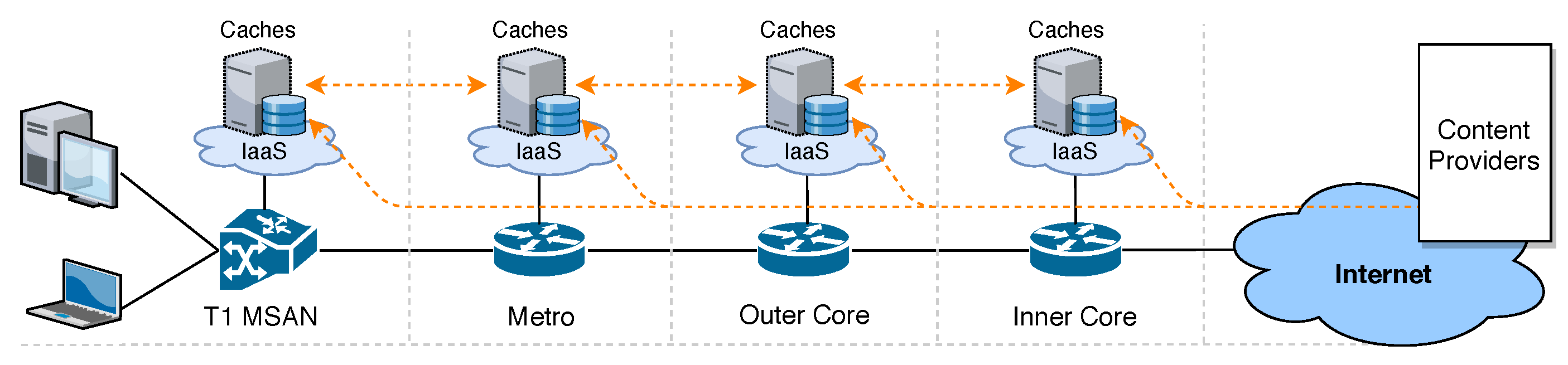
Figure 2.
Example datasets of cache workload.
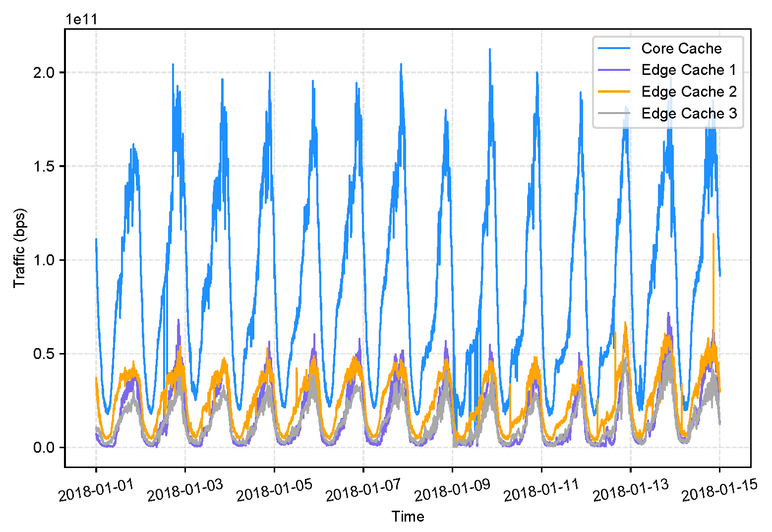
Figure 3.
A workflow of workload data collection - modeling - prediction - application scaling.
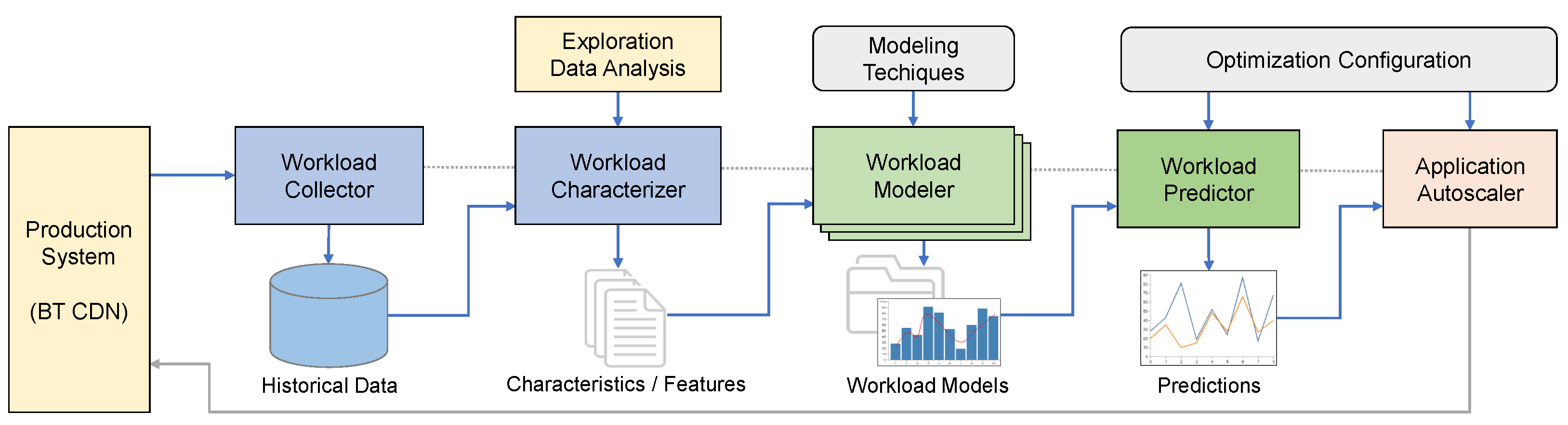
Figure 4.
A validation dataset and its sliding window
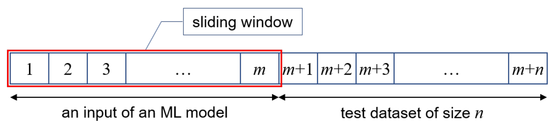
Figure 14.
An architecture of the workload prediction framework
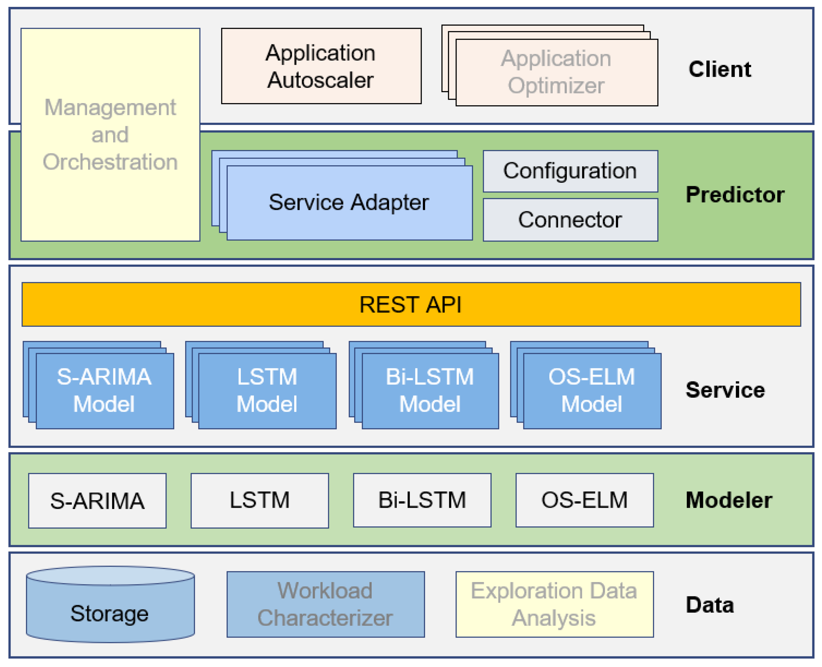
Figure 15.
Performance of the 1-hour ensemble model
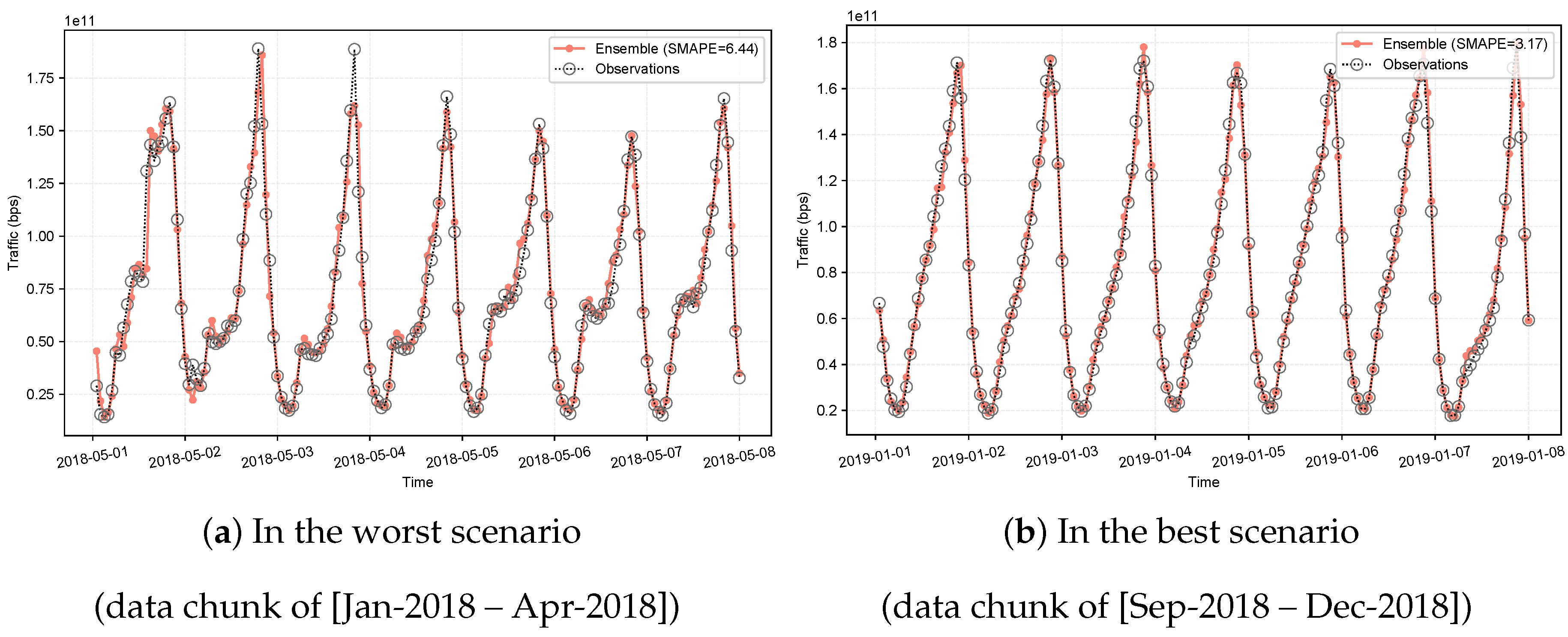
Figure 16.
Workload-to-resource transformation
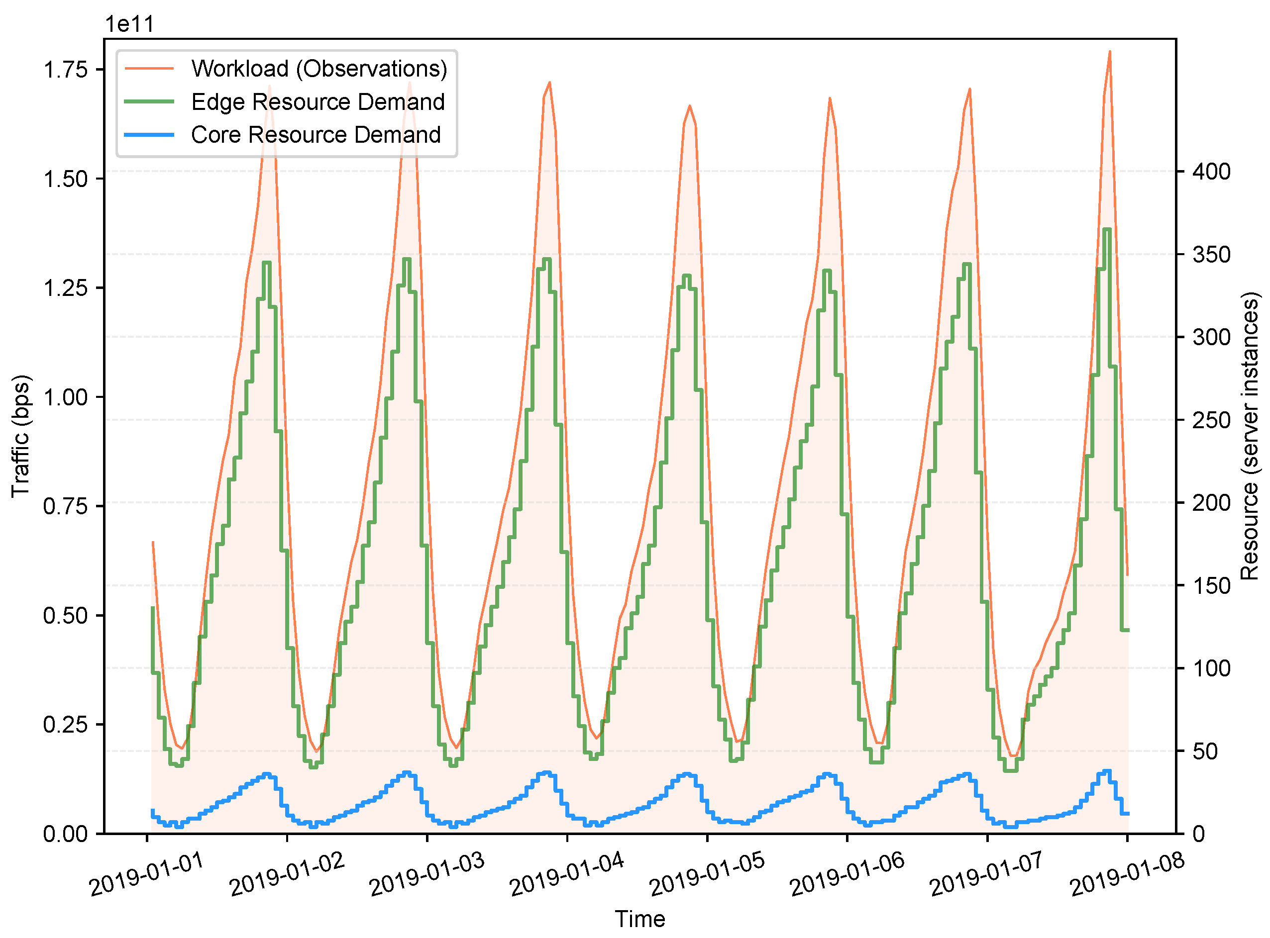
Figure 17.
Resource allocation based on workload prediction made by the 1-hour ensemble model of the best scenario.
Figure 17.
Resource allocation based on workload prediction made by the 1-hour ensemble model of the best scenario.
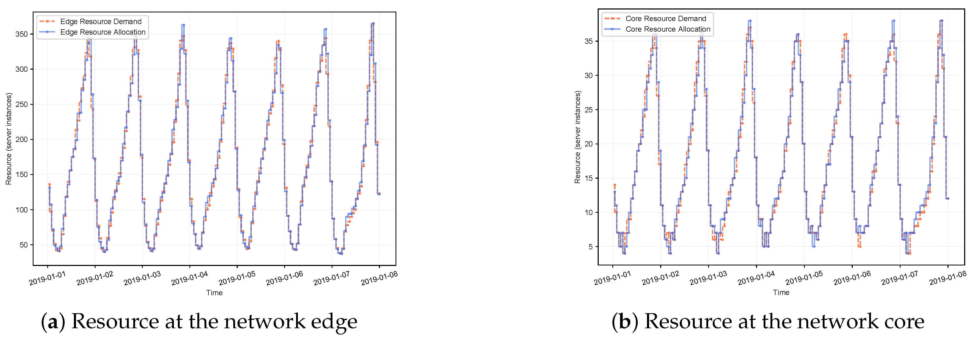
Figure 18.
Service rejection rates
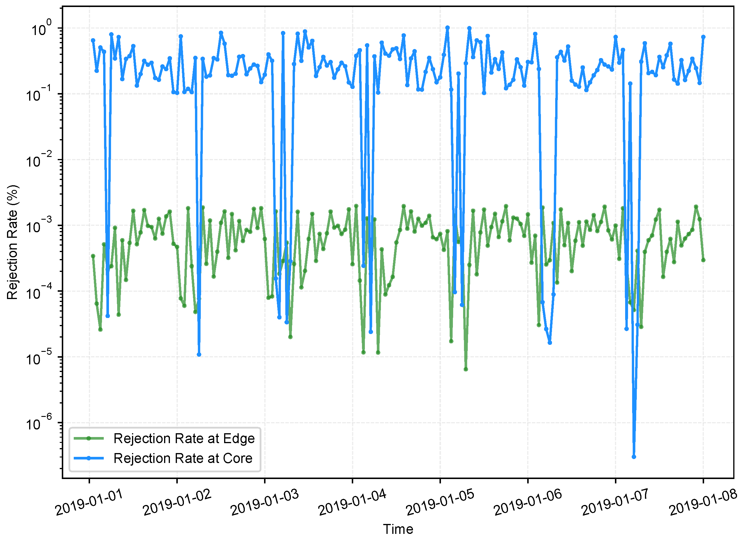

Table 1.
Prediction error (SMAPE) of the models
| Scenario | 10-minute models | 1-hour models | ||||
| S-ARIMA | Bi-LSTM | Ensemble | S-ARIMA | LSTM | Ensemble | |
| Best | 2.60 | 2.04 | 2.02 | 3.82 | 3.79 | 3.17 |
| Worst | 11.00 | 9.55 | 9.98 | 8.09 | 6.77 | 6.44 |
Table 2.
Parameters used in the workload-to-resource model.
| Parameter | Value | Description |
|---|---|---|
| Core server instance | ||
| 2.1 ms | Average serving time | |
| 50 ms | Maximum acceptable serving time | |
| Edge server instance | ||
| 21 ms | Average serving time | |
| 1700 ms | Maximum acceptable serving time | |
Disclaimer/Publisher’s Note: The statements, opinions and data contained in all publications are solely those of the individual author(s) and contributor(s) and not of MDPI and/or the editor(s). MDPI and/or the editor(s) disclaim responsibility for any injury to people or property resulting from any ideas, methods, instructions or products referred to in the content. |
© 2025 by the authors. Licensee MDPI, Basel, Switzerland. This article is an open access article distributed under the terms and conditions of the Creative Commons Attribution (CC BY) license (http://creativecommons.org/licenses/by/4.0/).
Copyright: This open access article is published under a Creative Commons CC BY 4.0 license, which permit the free download, distribution, and reuse, provided that the author and preprint are cited in any reuse.


