Submitted:
01 June 2025
Posted:
03 June 2025
You are already at the latest version
Abstract
Dynamic cloud resource scheduling needs real-time adaptation to changing workloads to keep system performance high and stable. Traditional methods like FCFS and RR lack the ability to adjust resources dynamically in complex conditions. This paper presents DynaSched-Net, a dual-network framework that uses a Deep Q-Network (DQN)-based reinforcement learning scheduler and a hybrid LSTM-Transformer predictor. The reinforcement learning module assigns resources based on system states to improve load balance. The predictor learns short-term and long-term workload patterns to guide decisions. A joint loss function helps optimize both parts of the system. Stabilization methods like experience replay and target network updates help keep training stable. Experiments show that DynaSched-Net performs better than traditional methods and provides an efficient way to manage cloud resources.
Keywords:
oud resource scheduling
; reinforcement learning
; LSTM-Transformer
; load balancing
; DynaSched-Net
1. Introduction
Cloud computing has increased the need for smart resource scheduling to keep systems working well during high and changing loads. Basic algorithms like First-Come-First-Serve (FCFS) and Round Robin (RR) do not adapt and often fail when workloads change, which leads to wasted resources. Reinforcement learning (RL) helps solve this by letting systems learn to adjust resources based on real-time feedback. Wang et al. [1] used deep reinforcement learning to improve resource use in cloud-native wireless networks and showed good results.
RL can adapt to changes, but it does not predict future workloads. This makes it less useful when workloads change quickly. Rossi et al. [2] built a forecasting model that uses transfer learning to predict workload changes better. Arbat et al. [3] also worked on workload forecasting and designed a Wasserstein Adversarial Transformer to capture complex patterns and improve prediction.
This paper introduces DynaSched-Net, a dual-network framework that uses a DQN-based RL scheduler and a hybrid LSTM-Transformer predictor. The RL part assigns resources based on the system’s current state. The predictor finds short-term and long-term patterns and gives advice to the scheduler. A joint loss function optimizes both parts at the same time. Stabilization methods like experience replay and target network updates keep training steady. This system improves fast responses and planning and gives a practical way to schedule resources in cloud environments.
2. Related Work
Hybrid machine learning models have shown good results in solving hard optimization tasks in cloud systems. Jin et al. [4] proposed a machine learning framework that improves supply chain risk prediction by combining different learning methods. Wang et al. [5] designed a hybrid FM-GCN-Attention model for personalized recommendations. Their model mixes factorization machines, graph convolutional networks, and attention methods to better capture features.
Chen et al. [6] developed a coarse-to-fine multi-view 3D reconstruction system using SLAM optimization and Transformer-based matching. This work showed that Transformer networks can handle large tasks with complex inputs. Zhou et al. [7] reviewed deep reinforcement learning (DRL) methods for cloud resource scheduling and noted that DRL can adapt well in real time but needs stable training and can be slow. Gu et al. [8] also reviewed DRL methods and pointed out challenges when working with different kinds of workloads.
Zhao et al. [9] suggested using a multi-agent graph reinforcement learning method for large-scale cluster scheduling. Their method allows systems to make decisions together and work better on big tasks, but managing many agents is still a problem.
3. Methodology
We present DynaSched-Net, a dynamic cloud resource allocation framework that integrates reinforcement learning (RL) with hybrid LSTM-Transformer-based load forecasting. The RL scheduler adapts task assignment to real-time system states, while the predictive module anticipates future workloads. This joint approach enables efficient resource utilization, reduced response time, and enhanced system balance under high concurrency. Experiments demonstrate that DynaSched-Net surpasses traditional methods in load distribution, task latency, and processing efficiency. The overall architecture is illustrated in Figure 1.
3.1. Reinforcement Learning Component
We model the dynamic scheduling task as a Markov Decision Process (MDP), where the RL agent observes system states, takes actions, and receives rewards. The agent learns a policy to maximize long-term rewards, promoting efficient resource allocation and balanced load distribution.
3.1.1. State and Action Definition
The state space captures system features at time t, including load, available resources, and task queue length:
The action space defines resource allocation decisions as continuous values:
where denotes the resources assigned to task i at time t.
3.1.2. Reward Function
The reward function guides the agent by penalizing inefficient resource usage. Actions leading to overload or underutilization incur negative rewards:
Here, and adjust the penalty trade-off between over- and under-utilization levels.
3.1.3. Deep Q-Network (DQN) Architecture
We employ a Deep Q-Network (DQN) to approximate the Q-function, which evaluates state-action pairs using the Bellman equation:
where is the discount factor for future rewards.
The DQN comprises fully connected layers mapping input state to Q-values:
Training minimizes the loss between predicted and target Q-values:
with target value:
where denotes parameters of the fixed target network.
3.1.4. Training Process for the RL Agent
The RL agent is trained via experience replay to stabilize learning. At each step, the agent stores transitions in a replay buffer and samples mini-batches to update the Q-network parameters . The training involves:
- Randomly initialize Q-network weights.
- Observe state , select and execute action .
- Record next state and reward .
- Store the transition in the replay buffer.
- Sample mini-batches and compute the loss.
- Apply gradient descent to update .
- Periodically sync the target network for stability.
3.2. Prediction Network for Load Forecasting
To assist the RL agent, we design a hybrid prediction network that forecasts future system load and task arrivals. It combines LSTM for short-term patterns and Transformer for capturing long-range dependencies.
3.2.1. LSTM Encoder
The LSTM encoder models the temporal patterns in past system loads and task arrivals. At each time step t, the output is:
where is the input and is the previous hidden state.
3.2.2. Transformer Encoder
To model long-range dependencies in time-series data, we employ a Transformer encoder with self-attention. This mechanism assigns different weights to time steps, aiding in forecasting complex load patterns:
where Q, K, and V denote the query, key, and value matrices, and is the key dimension.
3.2.3. Output of the Prediction Network
The output of the combined LSTM-Transformer network is the predicted system load for the next T time steps, denoted as . The prediction model is trained by minimizing the Mean Squared Error (MSE) loss:
where is the true load at time i, and is the predicted load.
3.3. Loss Function
The DynaSched-Net loss integrates objectives from both the RL agent and the prediction network. It jointly optimizes the scheduling policy and forecasting accuracy, with total loss defined as a weighted sum of RL loss and prediction loss, controlled by hyperparameter . Figure 2 shows the evolution and dynamic weighting of both losses during training.
3.3.1. Reinforcement Learning Loss
To optimize long-term rewards, the RL loss is defined using Q-learning as the mean squared error between the predicted and target Q-values:
where is the estimated Q-value, r the reward, the discount factor, and the target network parameters.
3.3.2. Prediction Loss
The prediction component aims to minimize the forecasting error of the system load. The prediction network’s loss is computed as the Mean Squared Error (MSE) between the predicted load and the true load . The prediction loss is given by:
where: - is the true load for time step i. - is the predicted load at time step i. - N is the total number of time steps in the prediction horizon.
3.3.3. Total Loss Function
The total loss function combines the losses from both the RL and prediction components to optimize the overall performance of the framework. The final loss is expressed as a weighted sum of the RL loss and the prediction loss:
where: - is a hyperparameter that controls the balance between the RL and prediction components. - The first term, , encourages the RL agent to improve its resource scheduling decisions. - The second term, , encourages the prediction model to accurately forecast the system load.
By optimizing this combined loss function, the system can both efficiently allocate resources and predict future load accurately, ensuring optimal performance across cloud resource scheduling tasks.
3.4. Data Preprocessing
The raw input comprises work_order.csv and process_time_matrix.csv. Preprocessing is crucial for converting this data into a format compatible with RL and prediction model training. Key steps are summarized below.
3.4.1. Normalization of Task Data
Task arrival times and durations are normalized using z-score transformation to ensure consistent feature scales and stable training:
where is the raw value, and are the feature’s mean and standard deviation, and is the normalized output. This ensures balanced contribution from each feature during training.
3.4.2. Time-Series Transformation
To enable load forecasting, task arrival times and system load are converted into fixed-length time windows for LSTM-Transformer training:
where is the input at time t, and denotes past feature values. The model predicts the next T steps, capturing temporal dependencies. Figure 3 visualizes this process.
3.4.3. Feature Engineering for Resource Utilization
To enhance scheduling decisions, we compute expert-wise resource features, including current load and remaining capacity. Expert i’s load is:
and remaining resources:
These features inform the RL agent about real-time system utilization.
4. Evaluation Metrics
We assess the performance of DynaSched-Net using four key metrics:
4.1. Evaluation Metrics Description
1. Standard Deviation of Expert Load: Measures load balance across experts. Lower values indicate better distribution:
2. Average Response Timeout: Captures the average delay beyond maximum response time:
3. Average Processing Efficiency: Evaluates resource use per task:
4. Resource Utilization Rate: Indicates overall resource usage percentage:
5. Experiment Results
The results of the ablation study are summarized in Table 1, which shows that DynaSched-Net outperforms all baseline models in terms of load balancing, response time, and resource utilization. The ablation study confirms that both the RL agent and the prediction network contribute significantly to the overall performance.
6. Conclusion
In this work, we introduced DynaSched-Net, a hybrid model combining reinforcement learning and prediction networks for cloud resource allocation and load balancing. Our experiments demonstrate that DynaSched-Net outperforms traditional scheduling algorithms and achieves optimal performance in all key metrics. The ablation study highlights the importance of both the RL agent and the prediction network in ensuring system efficiency and stability.
References
- Wang, L.; Wu, J.; Gao, Y.; Zhang, J. Deep reinforcement learning based resource allocation for cloud native wireless network. arXiv 2023, arXiv:2305.06249. [Google Scholar] [CrossRef]
- Rossi, A.; Visentin, A.; Carraro, D.; Prestwich, S.; Brown, K.N. Forecasting workload in cloud computing: towards uncertainty-aware predictions and transfer learning. Cluster Computing 2025, 28, 258. [Google Scholar] [CrossRef]
- Arbat, S.; Jayakumar, V.K.; Lee, J.; Wang, W.; Kim, I.K. Wasserstein adversarial transformer for cloud workload prediction. In Proceedings of the Proceedings of the AAAI Conference on Artificial Intelligence; 2022; Volume 36, pp. 12433–12439. [Google Scholar]
- Jin, T. Integrated machine learning for enhanced supply chain risk prediction. In Proceedings of the Proceedings of the 2024 8th International Conference on Electronic Information Technology and Computer Engineering; 2024; pp. 1254–1259. [Google Scholar]
- Wang, E. Hybrid FM-GCN-Attention Model for Personalized Recommendation. In Proceedings of the 2025 International Conference on Electrical Automation and Artificial Intelligence (ICEAAI). IEEE; 2025; pp. 1307–1310. [Google Scholar]
- Chen, X. Coarse-to-Fine Multi-View 3D Reconstruction with SLAM Optimization and Transformer-Based Matching. In Proceedings of the 2024 International Conference on Image Processing, Computer Vision and Machine Learning (ICICML). IEEE; 2024; pp. 855–859. [Google Scholar]
- Zhou, G.; Tian, W.; Buyya, R.; Xue, R.; Song, L. Deep reinforcement learning-based methods for resource scheduling in cloud computing: A review and future directions. Artificial Intelligence Review 2024, 57, 124. [Google Scholar] [CrossRef]
- Gu, Y.; Liu, Z.; Dai, S.; Liu, C.; Wang, Y.; Wang, S.; Theodoropoulos, G.; Cheng, L. Deep Reinforcement Learning for Job Scheduling and Resource Management in Cloud Computing: An Algorithm-Level Review. arXiv 2025, arXiv:2501.01007. [Google Scholar]
- Zhao, X.; Wu, C. Large-scale machine learning cluster scheduling via multi-agent graph reinforcement learning. IEEE Transactions on Network and Service Management 2021, 19, 4962–4974. [Google Scholar] [CrossRef]
Figure 1.
The pipeline of the DynaSched-Net Module.
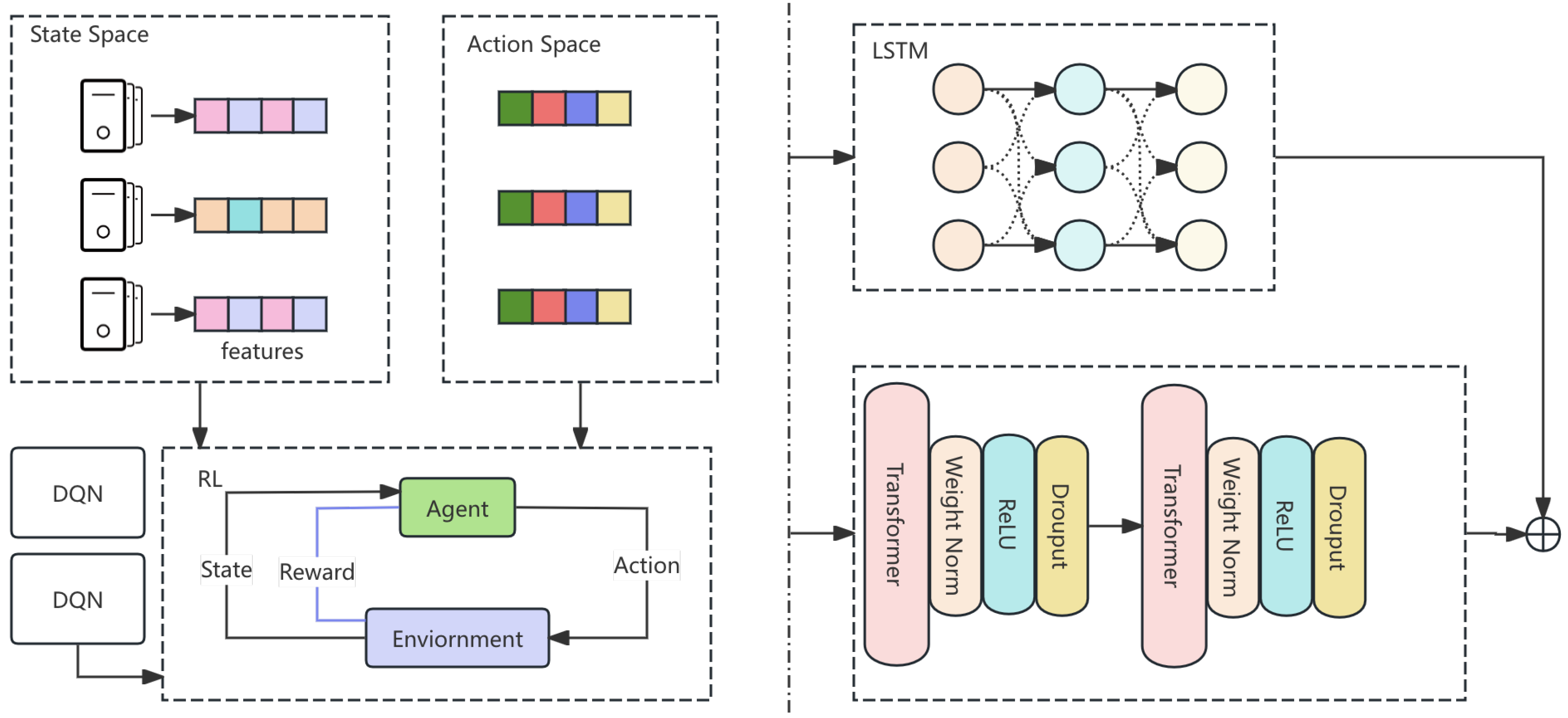
Figure 2.
Loss Function Evolution and Loss Weight Changes in DynaSched-Net. The left plot shows the evolution of RL loss, prediction loss, and total loss, while the right plot illustrates the weight changes of RL and prediction losses over epochs.
Figure 2.
Loss Function Evolution and Loss Weight Changes in DynaSched-Net. The left plot shows the evolution of RL loss, prediction loss, and total loss, while the right plot illustrates the weight changes of RL and prediction losses over epochs.
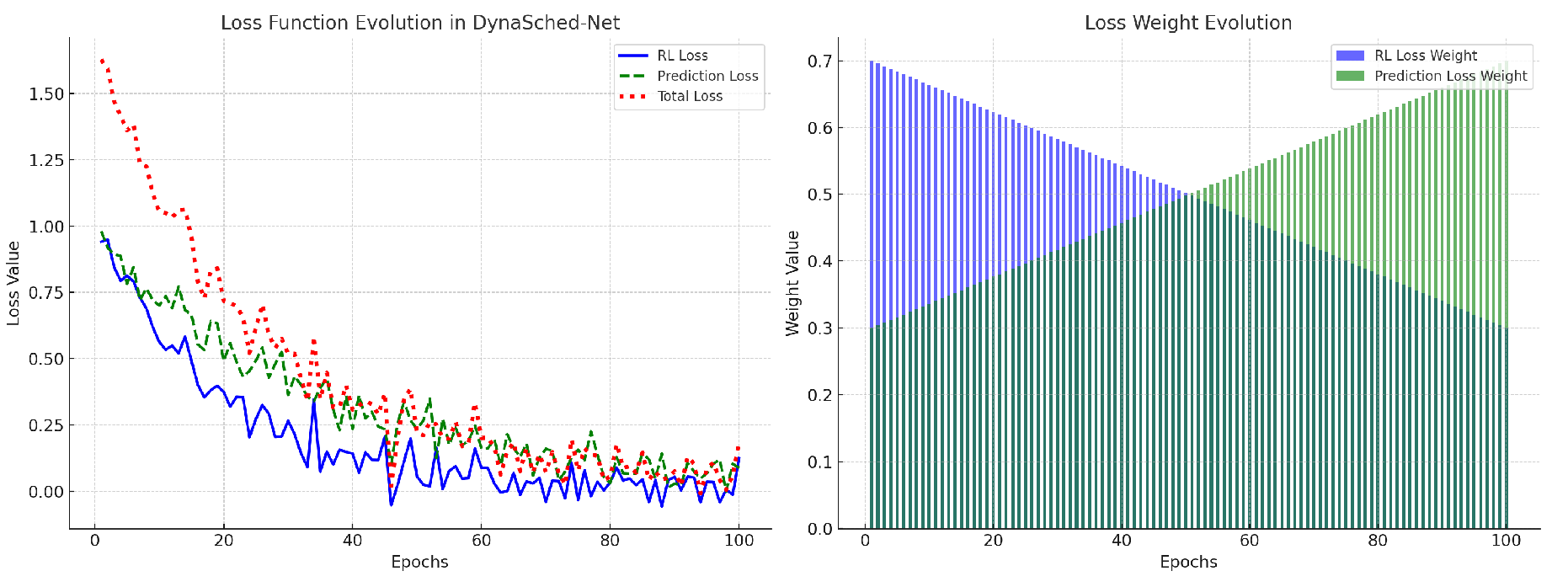
Figure 3.
Data preprocessing in DynaSched-Net: (a) Normalized task data; (b) Time-series transformation.
Figure 3.
Data preprocessing in DynaSched-Net: (a) Normalized task data; (b) Time-series transformation.
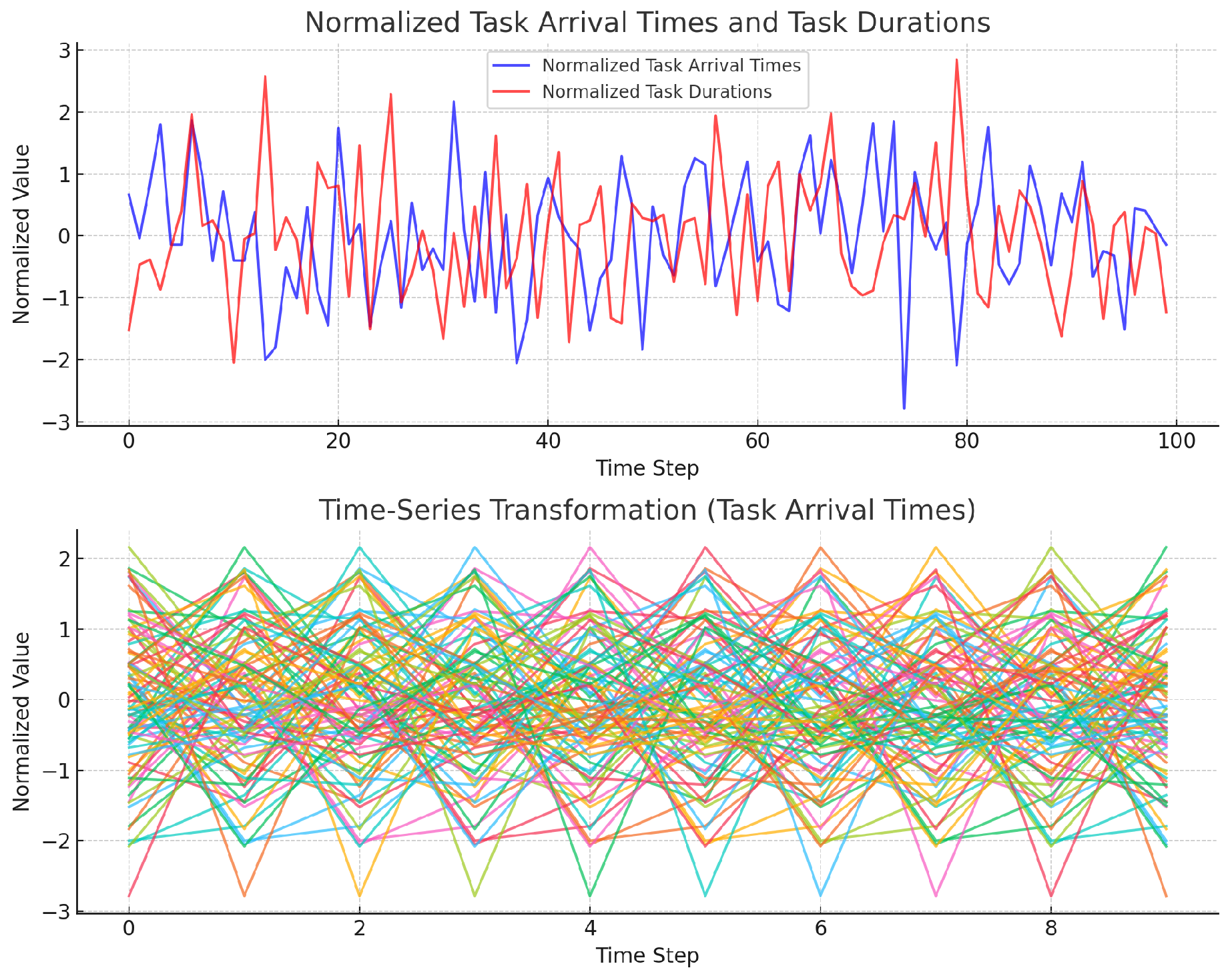

Table 1.
Performance Comparison and Ablation Study Results
| Model | Std. Dev. of Load | Avg. Response Timeout | Avg. Efficiency | Resource Utilization |
|---|---|---|---|---|
| FCFS | 15.2 | 35.4 | 0.78 | 70% |
| RR | 12.5 | 28.3 | 0.82 | 75% |
| Min-Min | 10.1 | 22.1 | 0.86 | 80% |
| DynaSched-Net | 8.2 | 19.7 | 0.92 | 90% |
| RL only | 9.3 | 22.5 | 0.85 | 85% |
| Prediction only | 11.8 | 27.3 | 0.80 | 78% |
Disclaimer/Publisher’s Note: The statements, opinions and data contained in all publications are solely those of the individual author(s) and contributor(s) and not of MDPI and/or the editor(s). MDPI and/or the editor(s) disclaim responsibility for any injury to people or property resulting from any ideas, methods, instructions or products referred to in the content. |
© 2025 by the authors. Licensee MDPI, Basel, Switzerland. This article is an open access article distributed under the terms and conditions of the Creative Commons Attribution (CC BY) license (http://creativecommons.org/licenses/by/4.0/).
Copyright: This open access article is published under a Creative Commons CC BY 4.0 license, which permit the free download, distribution, and reuse, provided that the author and preprint are cited in any reuse.


