
Submitted:
22 October 2025
Posted:
23 October 2025
You are already at the latest version
Abstract
As the IoT continues to grow, the need for efficient and effective task processing at the network’s edge becomes crucial. This thesis delves into leveraging DRL to enhance real-time task offloading in IoT edge computing, aiming to optimise resource utilisation and minimise latency. A novel approach is presented, combining BLSTM networks for predicting load and the A2C algorithm for making dynamic offloading decisions. This framework anticipates the load on MEC servers and strategically offloads tasks to balance computational demands. The research highlights significant contributions, including the implementation of BLSTM for precise load prediction by understanding temporal task request patterns and the use of the A2C algorithm to dynamically optimise offloading decisions based on these predictions and the current system state. Comprehensive experiments show that the proposed model surpasses traditional strategies, such as Deep Q-Networks (DQN), in maximising rewards and ensuring system stability. These findings underscore the potential of DR-based methods to significantly enhance IoT edge computing efficiency by achieving balanced and responsive task offloading, thus promoting the development of more intelligent and resilient IoT systems.
Keywords:
task offloading
; edge computing
; reinforcement learning
; internet of things
1. Introduction
The Internet of Things (IoT) has recently emerged as a significant development in IT, be- coming an essential part of our daily lives. IoT device’s function both as data producers and consumers, integrating seamlessly into current IT industries[1]. The number of interconnected IoT devices is expected to rise to 75.44 billion. However, these devices are limited by their battery, storage, and processing capabilities, leading to tasks being transferred to the cloud to enhance the quality of service (QoS)[2].
Fog/edge computing addresses these challenges by bringing storage and computing resources closer to end users, enabling resource-intensive tasks to be offloaded to nearby servers and enhancing IoT application efficiency. Edge computing leverages servers situated close to users[3]. With advancements in 5G, smart devices, and cloud computing, high-performance computing has progressed, and the data generated by IoT devices has exploded. emerging IoT applications are pushing the boundaries of data communication and processing requirements. These include Virtual Reality VR, AR, intelligent transportation systems, smart homes, and smart health systems. These ap- plications demand extremely low latency in both data transmission and computational requirement that traditional cloud computing models struggle to meet. The inherent delays in cloud-based systems make them inadequate for these time-sensitive IoT applications [4].
Mobile Edge Computing (MEC) brings user and edge servers closer, as illustrated in Figure 1. By transferring computation-intensive tasks to computation servers deployed at the user’s end, MEC reduces the backhaul traffic to distant cloud data centers, thus reducing the time required for time-sensitive applications and conserving energy. The offloading process involves making crucial decisions on which tasks to offload and determining the optimal location for the offloading process, directly influencing system QoS and performance. Scholars have suggested various innovative methods to im- prove offloading, including MDP-based, RL-based, and prediction-based approaches.
MEC offers computing services at the network edge, enabling real-time data analytics while preserving privacy, enhancing network capabilities, and alleviating congestion in backbone networks[6]. When IoT-generated data is sent to the cloud/fog/edge for processing, known as task offloading, conventional cloud computing faces challenges due to the distance between the Cloud Server (CS) and users, leading to significant load, congestion, and elevated transmission latency[2]. The deployment of many edge servers allows for collaboration and optimization of computing resources, enhancing task processing efficiency.
Edge computing, which provides computing capabilities at the network’s periphery, delivers improved response times and reduced latencies. Fog computing, on the other hand, furnishes computing, networking, and storage services to IoT devices using net- work devices within the Local Area Network (LAN) of the IoT devices. In contrast, edge computing uses small data centers near the IoT devices, facilitated by Wi-Fi access points, to minimize task completion times[7].
Task completion time, a crucial QoS metric, is measured from request submission to result reception and is influenced by waiting, transmission, and computation delays. For mobile devices with limited battery capacity, energy consumption is another critical factor, primarily affected by data processing and transmission. These elements are key considerations in assessing performance and efficiency, especially given the power constraints of portable devices. Effective computation offloading remains a challenge due to its NP-hard nature[2].
Reinforcement learning (RL) involves acquiring the optimal policy through exploratory and exploitative actions to maximize cumulative rewards. This sequential decision- making process is influenced by state changes and comprises key components like environment, agent, state, action, and reward[8]. However, RL algorithms often over- look the dynamic and foreseeable nature of task offloading, potentially leading to sub optimal decisions. Conventional approaches focus on static optimization, while deep reinforcement learning methods address dynamic IoT task computing but may neglect task inference testing, leading to notable response delays[9].
Decision-making in task offloading, determining the task whether offload to the remote server or compute locally, is crucial and merits thorough examination[2]. The decision typically involves addressing a multi-objective optimization problem. Common solutions include transforming multiple objectives into one objective or using one primary objective with others as constraints[2].
BLSTM, an advanced recurrent neural network (RNN), is capable of handling the vanishing gradient problem faced by RNNs and has been effective in forecasting user mobility[10]. LSTM shows promise for trajectory prediction[11]. In our approach, we integrate BLSTM into the A2C algorithm, creating the BLSTM-A2C algorithm, which enhances monitoring of user mobility and system utility. Policy-based RL directly models the policy guiding the agent’s behavior, with better learning convergence than value- based RL. However, policy-based RL faces slow learning convergence due to difficulty in determining optimal actions. To address this The A2C method proposes to addresses the strengths and weaknesses of both value-based and policy-based RL[12].
In this research, the main concern is to balance low latency and low energy consumption while decrease task drop rate and maximizing reward in real-time task offloading with mobility. We will consider an intelligent hybrid model combining BLSTM and A2C for dynamic real-time task offloading in edge computing systems serving IoT devices. This hybrid technique will consider computational constraints of IoT endpoints, applying quantization techniques to reduce computational requirements during training and inference, and adapting to changing network and computational states in real- time to optimize latency, energy consumption, and computational cost, while handling device mobility.
2. Methodology
This research utilizes Google cluster datasets to evaluate a BLSTM architecture for IoT task offloading and resource management datasets proposed in[13]. The dataset, released in 2011, contains 29 days of comprehensive cloud environment data, including information from 10,388 machines, over 670,000 jobs, and 20 million tasks, with details on task arrival times, data sizes, processing times, and deadlines. The data is organized across six separate tables, and to improve data quality and usability, the researchers performed preprocessing steps, notably converting time measurements from microseconds to seconds, while addressing common challenges like noise, inconsistency, and missing data in the raw dataset.
Time(s) = Time(s)x106
- System Model
The proposed framework employs a Deep Reinforcement Learning (DRL) agent to optimize task offloading in a Mobile Edge Computing (MEC) environment, as shown in Figure. 2. The system consists of N mobile devices and M MEC servers connected to a macro–Base Station (BS) via fiber cables, with the DRL agent centrally managing task distribution based on historical performance patterns. The agent aims to minimize system cost and task drop rates while maximizing rewards by analyzing server load patterns and predicting capable nodes based on their CPU and memory resource history. The MEC servers, co-located with the macro-BS and Small Base Stations (SBSs), are responsible for collecting, processing, and delivering results for computation tasks submitted by mobile devices within specified time slots, with the goal of achieving optimal cost efficiency and reduced latency for time-sensitive data.
- 1)
- Task Model
IoT devices generate tasks across different time slots, represented as T = (1, 2, 3, . . ., Tn), with arrival times and data sizes based on real-world IoT data. Each task is initially sent to the Helper MEC with relevant task and device information. The decision model then determines whether to offload the task to the MEC server or process it locally. In a given time slot t ∈ T, a new task generated by IoT device n ∈ N is characterized by the tuple , , , B, where is the task data size, is the required computational resources per bit (in CPU cycles/bit), ( B ) is the task’s communication bandwidth, and is the maximum tolerated delay to meet QoS demands. If the task isn’t completed by the end of time slot , it’s discarded.
- 2)
- Decision model
When a new task arrives for MD n ∈ N at the start of time slot t ∈ T, an optimal offloading decision is required. We use a binary variable to represent this decision: indicates local processing, while signifies offloading to an edge node. The decision model’s role is to determine this offloading scheme optimally.
The decision model will provide the offloading scheme for this task.
In our model, IoT devices generate tasks in real-time. Each task is considered atomic, it cannot be divided or split into smaller parts. This indivisibility is a key characteristic that influences the offloading decision process.
- 3)
- Channel /communication Model
Our system, depicted in Figure 2, features MEC nodes distributed across various regions. This infrastructure includes multiple APs, edge servers, and N MDs, indexed as n= (1,2,3, . . ., N). MDs connect to the MEC through either APs or mobile networks. The macro-BS must determine the optimal task offloading location within the network, considering factors such as edge server workload, response time, latency, and energy consumption.
The utilization of resources and the introduction of transmission delays occur exclusively when the task is offloaded to the edge server for execution. The offloading of the task is denoted as where BNM represents the corresponding bandwidth allocation, consisting of This task offloading is governed by the bandwidth constraint, signifying that must be less than or equal to , which is further constrained by Utilizing Shannon’s formula enables the determination of the transmission rate[14].
In the context provided, the channel gain of between MD and the AP is represented by g and representing a distance from the MD and the nearest AP., and the power of additive Gaussian white noise is denoted by . We define as the distance between MD n and MEC server m, where denotes the current location of m and is the location of m[15]. Consequently, the equations allow for the derivation of the task’s transmission delay and transmission energy consumption.
we set, where Pmax is the maximum transmit power when the battery.
- 4)
- Computation Model
Computation time, measured time duration from request to submit result, it is a key QoS metric in offloading design. It’s affected by waiting, transmission, and processing delays. Energy consumption, crucial due to limited device batteries, includes data processing and transmission costs[8].
- a)
- Local Execution
Processing a task locally on a device incurs both a time delay and power consumption. If we denote the processing capacity of the IoT device as , then the processing delayfor task m on MD n can be calculated using Equation 5. These factors contribute to the overall cost of local task execution and play a crucial role in decision-making for task offloading.
Similarly, the energy consumption for task m of user n during local computation is denoted by and is defined by Equation 6. This equation captures the power consumed during the local execution of the task.
where , denotes the energy consumption and the power coefficient, which depends on the chip architecture[16] respectively when the task is processed in the MD. Therefore, the computational cost is characterized as the weighted aggregate of both the energy consumed and the time taken for the completion of a task assigned to node n. The overall cost is then computed as the weighted sum of local costs in the subsequent manner as shown in Equation 7.
Where α and β are constant weighting parameters corresponding to the time and power consumption of the task λnm and the sum of weights is always equal to 1, α + β = 1 and must fulfill 0 <= α <= 1 and 0 <= β <= 1. In this scenario, diverse user requirements can be accommodated through the adjustment of weights. For instance, prioritizing over indicates a higher emphasis on minimizing delay rather than energy consumption, making it suitable for latency- sensitive applications.
- b)
- Algorithm for calculating local cost
Algorithm 1, which calculates the local cost, begins by setting the initial action for each device to local computationand the system’s total cost to zero . Following this initialization phase, the algorithm takes several parameters as input. These include the size of computation , the number of CPU cycles required ) the local computation power of the device and the decision weights (α and β). These parameters are used to determine the cost of local computation for each device.
| Algorithm 1: calculate the cost |
| Require: N, , , , , α, β, |
| Ensure: |
| 1: ← 0 ▷ Set total system cost |
| 2: for n ∈ N do |
| 3: ▷ time to execute |
| 4: ← ▷ energy consumption |
| 5: ← ( ▷ Calculate cost |
| 6: ← + ▷ Update the cost |
| 7: end for |
| 8: return |
- c)
- MEC Execution
When the decision unit opts to offload a task to an edge server (represented by ), it does so because the edge server’s computational resources significantly surpass those of the MD. The processing time per task on the edge server is denoted as , which encompasses both transmission and computing delays. The computing delay is influenced by factors such as the edge server’s CPU frequency and other available resources. It’s important to note that in this study, we make the assumption that the size of the computed results is minimal. Consequently, the time required to download these results from the MEC server is considered negligible. Given these conditions, the processing time can be expressed using equation 8.
Similarly, the corresponding power cost for task of user n is denoted by and is defined as equation 10.
Where is the power coefficient, The total system cost in edge computing is derived from two primary factors: the time required for computation and the associated power consumption. This can be expressed as:
The overall expense, denoted as , to calculate a task send from device n can be formulated as...
where is considered when the is not guaranteed when doing offloading.
Table 1 provides a comprehensive summary of the key notations used consistently throughout this paper.
- 5).
- Prediction Model
Traditional RL-based task offloading systems make decisions reactively, leading to potential delays and failures. By analyzing historical patterns of task generation, server usage, and mobile device movements, our system can predict future resource needs and pre-allocate computing resources to optimal MEC nodes before tasks arrive, significantly reducing decision-making delays and task failures.
- 6).
- Task Load Prediction Model
Using a trained LSTM model, our system predicts future task data by analyzing historical task sequences D1, D2, D3, from mobile devices. The model aims to minimize prediction error, enabling proactive resource allocation and service package loading before tasks arrive. and prediction of future MEC server loads using an LSTM model trained on historical CPU utilization data sequences H1, H2, .
The model outputs predicted server loads , identifying potentially idle servers
that can be prioritized for task offloading, thus preventing workload imbalances and enabling more efficient resource allocation decisions.
- B.
- Offloading Algorithm Design
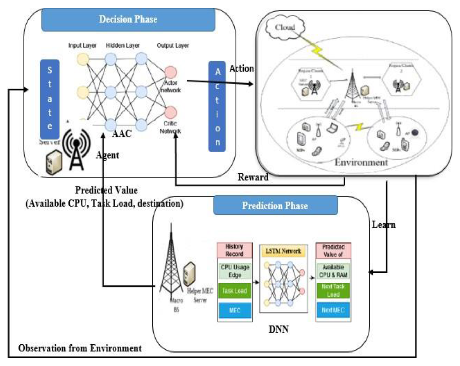
To dynamically adjust to changing conditions and make optimal choices, we’ve developed an innovative decision-making solution that combines two powerful techniques: BLSTM from deep learning and A2C from reinforcement learning. This integration results in a DRL based approach for task offloading, designed to anticipate and respond effectively to environmental shifts.
- 1).
- Prediction phase (BLSTM)
During the Prediction Phase, as illustrated in Figure 3, the algorithm forecasts future conditions such as CPU availability, upcoming task loads, and the nearest edge node. Upon arrival of an actual task, the system compares the predicted values with the real data for CPU, task, and node. If the discrepancy falls within an acceptable range, the task is offloaded to the location determined by the DRL Agent in the Decision Phase. However, if the error exceeds the set threshold, the Decision Phase reevaluates the offloading decision using the actual values. This new information is then incorporated into the historical dataset for future training. The training process of the BLSTM Net- works involves adjusting weights and biases to improve prediction accuracy.
- 2).
- Decision Phase (A2C)
Each IoT device generates various tasks at different times, and when a new task is created, there is a delay in the system’s response to the decision request for that task. To optimize performance, the system uses information from a prediction phase before it receives real task information. A DRL model called A2C is used to make offloading decisions for newly arrived tasks. The A2C network consists of two sub-networks: an actor and a critic, with shared layers to simplify the model and speed up network convergence. The network structure of the model is shown in Figure 3.
The edge server within A2C-BLSTM-based algorithm functions as a smart brain, where a RL agent interacts with the environment to learn optimal policies. The agent consists of two components: an actor, which defines a policy and performs actions based on observed states, and a critic, which evaluates the current policy and updates its parameters based on rewards from the environment[17].
The A2C algorithm initializes an actor to interact with the environment, using BLSTM networks to predict system parameters and select actions based on policies. After executing actions, the algorithm captures states and rewards in a replay buffer for iterative learning. A critic network estimates the advantage function to evaluate the actor’s decisions, and both the policy and critic networks are refined through gradient-based optimization to improve decision-making and maximize cumulative rewards within the A2C ecosystem.
Figure 4.
Decision Phase of A2C Network.
- C.
- DRL Decision model Elements
- 1)
- Environment State S
The state describes the environment and changes when the agent generates an action. In this model, each state consists of five pieces of information: task size (in bytes), deadline (in milliseconds), processing queue of the MD, transmission queue, and MEC processing queue information (all in bytes), and communication type (5G or Wi-Fi). The state is characterized as follows:
where is the task size, denotes the historical load level on each edge node, is the task deadline, and represent the processing state of devices, the transmission state of devices, and the MEC node state information for time slot t - 1, respectively. Additionally, represents the transmission rate of the MD.
- 2).
- Action a
The action space of this model comprised as a binary
Where N represents the computation server, and determines whether a task is processed at the MEC or locally. Specifically, is local when , and N is one of the MEC servers {1, 2, ..., M} when . The agent will make decisions based on the task offloading strategy at each time step and receive rewards from the environment in the subsequent time step. When local and MEC processing are both possible, the choice should optimize either latency or energy efficiency. If neither option is suitable, the task should be discarded.
- 3).
- Reward
After the agent executes an action, the reward serves as the environment’s feed- back to the agent. This reward, a numerical value, reflects the agent’s performance; at each time step (t + 1), the agent receives the reward and information about the updated state from the environment. Based on this feedback, the agent learns a policy (π), which is considered optimal () when consistently yielding the highest rewards. In this section, the costs and rewards are quantified based on local processing, remote processing, and task dropping to execute task λ(n). For every action, the system must choose between executing the task locally or offloading it to external resources.
α and β are weighting coefficients that balance the importance of processing time against energy consumption. represents the penalty cost for exceeding the allocated time.
Equation 15 is applied to choose a minor action with lower cost value for all multi- devices capable of processing data locally and remotely. if the allocated server is wrong or busy, that task will be discarded. The cost associated with discarding the task is denoted as , with a fixed value of 1. If the processing time surpasses the deadline, the algorithm imposes . In time-sensitive systems, tasks are evaluated against predetermined deadlines. Those exceeding these limits may be discarded to maintain overall system efficiency. While minor delays are of- ten tolerable, the acceptable threshold varies based on task type and criticality. A penalty system quantifies the cost of delays, helping to prioritize timely task completion and optimize resource allocation. This approach balances the need for thorough processing with the demands of real-time responsiveness across diverse application scenarios. The penalty for breaching the deadline is defined as:
When a task meets its deadline, becomes 0, having no impact on the cost. However, for tasks exceeding the deadline, a penalty is applied using a squared function, which amplifies the effect of larger delays. To address the negligible impact of delays less than 1 second due to the squaring effect, time calculations in this range are processed in milliseconds. For instance, a 0.1second delay translates to a value of 10,000ms rather than 0.01. This approach ensures that even small delays contribute meaningfully to the penalty calculation. For offloading tasks , the costs and are calculated using Equations 17 and 18, respectively. These equations account for the specific characteristics of edge processing and its associated penalties.
At each time slot t, the agent is given an immediate reward for choosing action A. Typically, this reward function is inversely related to the cost function. The primary objective of the optimization problem is to minimize overall costs.
The objective of this research is to simultaneously reduce costs and increase re- wards, optimizing the system’s overall performance and efficiency.
- D.
- Prediction Based Decision Task offloading framework
Our algorithm combines A2C (Actor-Critic) with BLSTM (Bidirectional Long Short-Term Memory) to optimize task offloading in MEC environments. The system makes offloading decisions based on both predicted and actual server loads, choosing between edge processing and local execution. With probability ϵ, the agent selects minimum- cost actions; otherwise, it follows predicted or mathematical solutions with probability 1 − ϵ. The optimal policy minimizes the expected long-term cost: , where the total reward is calculated as The model continuously updates through policy gradients and advantage estimates, improving its decision-making capabilities over time.
| Algorithm 2: Proposed A2C-BLSTM-Based Task Offloading Decision Algorithm |
| 1: Input: Task in each time slot |
| 2: Output: Optimal offloading decision and total cost |
| 3: Initialize: |
| 4: Actor-Critic model and related parameters (γ) |
| 5: LSTM model for task prediction |
| 6: Error threshold ϵ |
| 7: Maximum tolerance time ψ |
| 8: for episode e = 1 to M do |
| 9: Initialize sequence s sequence |
| 10: for time slot t = 1 to T do |
| 11: Predict Load BLSTM |
| 12: Predict Task |
| 13: Wait for Real task (n) |
| 14: With probability 1 − ϵ, select mathematical A or predicted A |
| 15: δ =real task load ▷ real task load |
| 16: if δ > ϵ then |
| 17: for each m = 1 to M do |
| 18: [m]= |
| 19: end for |
| 20: |
| 21: if ≤ ψ then |
| 22: ▷ Select the edge server with minimum load |
| 23: else |
| 24: ▷ Select to process the task locally |
| 25: end if |
| 26: else |
| 27: Select → Predic Action (, ) |
| 28: if Predic Action ≤ ψ then |
| 29: = selected ▷ Select the edge server to processed the task |
| 30: else |
| 31: ▷ Select to process the task locally |
| 32: end if |
| 33: end if |
| 34: Execute action at (local or MEC) |
| 35: Calculate the cost of the action taken: |
| 36: if then |
| 37: Calculate local cost: ▷ Eq. 15 |
| 38: else |
| 39: Calculate MEC cost: ▷ Eq. 17 |
| 40: Receive reward = ▷ Reward is the negative cost |
| 41: Observe next state |
| 42: Calculate advantages: |
| 43: +V () |
| 44: Update Critic: Minimize |
| 45: Update Actor: Use policy gradient |
| 46: end for |
| 47: end for |
- 2.
- Experimental Result and Discussion
We use PYTHON simulation to evaluate the performance of our proposed algorithm. The A2C-BLSTM algorithm is conducted using Keras plus TensorFlow[18], where Keras is adopted to build the DNN training model and TensorFlow supplies the back- ground support. We utilize a dataset from Google Cluster[13], which contains details about task arrival times, data sizes, processing times, and deadlines of the task. Tasks vary from complex big data analysis to simpler image processing, each with unique processing requirements and data volumes. We preprocess and normalize the data based on task characteristics to ensure compatibility with our model, accounting for the interrelation between processing density, time, and data size across different task types. Based on similar research in the field[13,19,20], the authors have recommended and used specific simulation parameters to evaluate task offloading solutions. Accordingly, we have adopted and simulated their recommended parameters, as shown in Table 2
- Training process of BLSTM & DRL
Figure 5 shows that the model that used to predict the task load and CPU usage is well fitted, the LOSS decreases for larger epoch values hence it shows how the model starts to optimize properly heavily for a larger epoch. The model learns any pattern or context and adapts the workload fluctuation. This will lead to that out validation LOSS will decrease for longer epochs.
Prediction on Historical Data from the Google Cluster Dataset
The proposed model demonstrates strong predictive accuracy when compared against actual values using a historical data dataset and is applied to authentic cloud data sets, significantly impacting accuracy and performance. Figures 6a and 6b illustrate the prediction outcomes of the BLSTM model, contrasting actual data (blue line) with predicted data (orange line). The close alignment between the two lines (actual and predicted) in these figures indicates the robust fit of the proposed model.
- B.
- Discussion on Performance Comparison
To evaluate the performance of our A2C-BLSTM-based scheme in real-time for IoT, we compared our model with three benchmark algorithms: MADDPG[21], MAAC-based algorithm[17], and DQN-based algorithm[22]. We trained our model and the other three algorithms simultaneously in the same environment, including A2C-BLSTM with prediction and A2C without prediction.
These benchmark algorithms are commonly employed in MDP scenarios. The DQN algorithm operates as a single agent for dependent computation offloading, while MAD- DPG represents a state-of-the-art Multi-Agent Deep Reinforcement Learning (MADRL) framework. The MAAC algorithm, like our approach, utilizes a multi-agent reinforcement learning strategy based on the actor-critic method. Our comparison focused on key performance indicators: task drop rate, energy consumption, and task execution delay. To assess prediction accuracy, we employed Mean Squared Error (MSE), Mean Absolute Error (MAE), and Mean Absolute Percentage Error (MAPE). For optimization evaluation, we examined total system cost, total reward, and task throughput volume. The experimental setup involved eight edge servers and 80 terminal devices. As illustrated in Figure 6, our model consistently outperformed the benchmark methods across all metrics. This superior performance can be attributed to the model’s effective integration of predictive and decision-making techniques, which optimally utilize task characteristics and edge server load information.
- 1)
- Impact of Task Number
Previous studies have demonstrated that the task arrival rate significantly affects the system state due to the random generation of tasks. In this paper, we utilize data from real scenarios for data streams. Unlike traditional approaches that rely on task arrival rates to evaluate the system state, our study uses different time slots to assess the impact of the number of tasks on system cost, average task delay, and task discard rate.
Specifically, we set the time slots in the dataset to T = 0, T = 100, 200, and 500 and compare the performance of MADDPG, MAAC, DQN, and our A2C-BLSTM scheme under these different time slots. The experimental results are presented in Figure 7.
Figure 7a presents a comprehensive comparison of the task rejection ratios across four different schemes. As the number of tasks increases, the rejection ratio for all schemes also rises. However, our scheme demonstrates a significantly lower increase compared to the other schemes, indicating better performance in terms of task acceptance ratio and a lower rejection rate. The proposed model’s ability to accept more tasks stems from its intelligent assignment of tasks to servers that are optimally matched in terms of resource requirements and availability. This approach not only preserves resources for future use but also allows for more tasks to be accepted, reducing the overall time to complete tasks, which is a critical factor for real-time communication scenarios. A high acceptance rate is beneficial as it leads to higher resource utilization and reduces system idle time. Consequently, our proposed work outperforms other methods in terms of cost (latency and power consumption), demonstrating its effectiveness in improving the proposed MEC system.
The task throw rate is a crucial metric directly impacting QoS. A low task rejection ratio indicates high QoS. The proposed A2C-BLSTM-based scheme employs a robust mechanism for selecting the best servers by assessing CPU usage and task requirements, thereby enhancing the efficiency of the MEC system. Additionally, it leverages intelligent resource allocation strategies, resulting in an increased task acceptance rate while maintaining QoS. A higher acceptance rate typically leads to higher average resource utilization relative to cost. The results demonstrate that our model achieves a higher utilization rate than other algorithms, underscoring the effectiveness of the proposed approach in improving MEC system performance.
Figure 7b also presents a comprehensive comparison of the cost ratios of three different schemes as the number of tasks increases. It can be observed that the cost ratio for all schemes increases with the number of tasks. However, the proposed scheme exhibits a significantly lower increase compared to the other schemes, indicating better performance in terms of cost ratio. Additionally, it has a significantly lower task rejection rate compared to the MADDPG, MAAC and DQN algorithms, implying that it accepts more tasks for offloading and enhances the QoS of the MEC system. The key factor enabling the proposed one to achieve this is its ability to intelligently assign tasks to servers that are optimally matched in terms of resource requirements and availability, thus minimizing overall cost and maximizing resource utilization of the MEC system.
- 2)
- Impacts of Max tolerable time
Figure 8a illustrates our system’s performance across varying maximum tolerance latencies and algorithm configurations. The data reveals an inverse relationship between maximum tolerance latency and task drop rate for all four methods tested. As the tolerance increases from 5 to 30 seconds, task drop rates decrease markedly. Our proposed A2C-BLSTM algorithm consistently maintains a lower task drop rate compared to its counterparts. This advantage is particularly pronounced at lower maximum tolerance latencies, highlighting our algorithm’s efficacy for time-critical tasks. Conversely, Figure 8b demonstrates that average system latency increases for all methods as maximum tolerance latency extends from 5 to 30 seconds. This trend is attributed to task completion dynamics: at shorter tolerance levels, many tasks fail to complete, whereas longer tolerances allow more tasks to be processed and transmitted, resulting in higher aver- age system latencies.
- 3)
- Impacts of Prediction
The newly generated tasks demand optimal allocation of computational resources, which is achieved through a decision model. From the moment of task generation until the al- location decision is made, these tasks experience queuing and decision response delays within the cache queue. Our system employs a BLSTM prediction model to forecast incoming tasks based on historical data. This prediction then feeds into the decision model, which proposes an offloading scheme for task assignment. For the purpose of our experiment, we analyze the performance using the first 500 tasks generated. This approach combines predictive modeling with decision-making to optimize resource allocation and task management in a dynamic computational environment.
The results depicted in Figure 9 considerable advantages of utilizing prediction in task execution, comparing total task drop rate and system cost when doing prediction with the pro- posed algorithm and with just only implementing A2C without BLSTM prediction for decision making. Both graphs show a linear increase in task drop and cost as the number of tasks grows, but these increases are significantly steeper without prediction. The blue lines, representing execution without prediction, indicate higher task drop and costs than the orange lines, which represent a BLSTM prediction based A2C decision making to offload and a predicted resource allocation. Using prediction reduces both tasks drop rate and system cost, resulting in more efficient and cost-effective task management. These benefits become increasingly pronounced with a higher number of tasks, underscoring the scalability and strategic importance of predictive mechanisms in task management.
When comparing the results of prediction-based approaches versus those without pre- diction, it is evident that our method performs significantly better overall. However, our scheme requires additional energy initially to train the model until it reaches an error-tolerant threshold during prediction. This increased energy consumption occurs only during the initial deployment and training stage. Additionally, the training process is conducted on the MEC server and macro base stations, ensuring that this initial energy expenditure does not significantly impact the overall performance of the system.
Once the model is trained and deployed, the energy requirements stabilize, and the benefits of the prediction-based approach become more pronounced. These benefits include improved task offloading efficiency, reduced latency, and higher system reliability. By leveraging the computational resources of the MEC server and macro base stations, we ensure that the end-user experience remains unaffected during the training phase. This strategic deployment of training processes helps maintain optimal system performance while reaping the long-term advantages of our enhanced predictive model.
3. Conclusion
This study addresses the critical challenge of task offloading and resource allocation in mobile edge computing (MEC) environments, focusing on minimizing energy consumption and response times while maintaining high-quality real-time performance. By framing the problem as a Markov Decision Process (MDP) and employing an innovative Actor-Critic (A2C) algorithm integrated with BLSTM prediction, we developed an intelligent offloading strategy for mobile IoT devices. Simulation results confirm that the proposed approach outperforms traditional methods, achieving lower system costs, higher task acceptance rates, and improved resource utilization, ultimately enhancing the quality of service (QoS) for end-users.
Future research should focus on extending the A2C-based model to handle the dynamic mobility of devices in MEC environments. Developing algorithms that adapt to rapid changes in device locations and network conditions will be critical for seamless task offloading. Additionally, incorporating advanced AI techniques like federated learning, meta-learning, and enhanced predictive models can further optimize resource allocation and task scheduling, paving the way for more robust and efficient MEC systems.
References
- Y. Bin Zikria, R. Ali, M. K. Afzal, and S. W. Kim, “Next-Generation Internet of Things (IoT): Opportunities, Challenges, and Solutions,” pp. 1–7, 2021.
- S. Hossain, C. I. Nwakanma, J. M. Lee, and D. Kim, “Edge computational task offloading scheme using reinforcement learning for IIoT scenario,” ICT Express, vol. 6, no. 4, pp. 291–299, 2020. [CrossRef]
- H. Lin, S. Zeadally, Z. Chen, H. Labiod, and L. Wang, “Jo ur l Pr e r f,” J. Netw. Comput. Appl., p. 102781, 2020. [CrossRef]
- T. Kim and S. Yoo, “Edge / Fog Computing Technologies for IoT Infrastructure II,” pp. 2–4, 2023.
- M. Pendo, J. Mahenge, C. Li, and C. A. Sanga, “Energy-ef fi cient task of fl oading strategy in mobile edge computing for resource-intensive mobile applications,” Digit. Commun. Networks, vol. 8, no. 6, pp. 1048–1058, 2022. [CrossRef]
- W. Sun, J. Liu, and Y. Yue, “AI-Enhanced Offloading in Edge Computing : When Machine Learning Meets Industrial IoT,” no. October, pp. 68–74, 2019.
- J. P. Jue, “All One Needs to Know about Fog Computing and Related Edge Computing Paradigms All One Needs to Know about Fog Computing and Related Edge Computing Paradigms : A Complete Survey,” no. February, 2019. [CrossRef]
- L. Yan, “A Task Offloading Algorithm With Cloud Edge Jointly Load Balance Optimization Based on Deep Reinforcement Learning for Unmanned Surface Vehicles,” IEEE Access, vol. 10, pp. 16566–16576, 2022. [CrossRef]
- Y. Tu, H. Chen, and L. Yan, “Task Offloading Based on LSTM Prediction and Deep Reinforcement Learning for Efficient Edge Computing in IoT,” pp. 1–19, 2022.
- R. Li, C. Wang, Z. Zhao, R. Guo, and H. Zhang, “The LSTM-based Advantage Actor-Critic Learning for Resource Management in Network Slicing with User Mobility,” vol. 7798, no. 1, pp. 1–5, 2020. [CrossRef]
- C. Wang, L. I. N. Ma, R. Li, and H. Zhang, “Exploring Trajectory Prediction Through Machine Learning Methods,” pp. 101441–101452, 2019.
- T. Haarnoja, H. Zhu, G. Tucker, and P. Abbeel, “Soft Actor-Critic Algorithms and Applications,” 2015.
- H. Yuan et al., “Online Dispatching and Fair Scheduling of Edge Computing Tasks : a Learning-based Approach,” vol. 4662, no. c, 2021. [CrossRef]
- J. Wang, K. Liu, M. Ni, and J. Pan, “Learning Based Mobility Management Under Uncertainties for Mobile Edge Computing,” no. 1, pp. 1–6.
- Y. Miao, G. Wu, M. Li, A. Ghoneim, and M. Al-rakhami, “Intelligent task prediction and computation offloading based on mobile-edge cloud computing,” Futur. Gener. Comput. Syst., vol. 102, pp. 925–931, 2020. [CrossRef]
- V. D. Tuong, T. P. Truong, T. Nguyen, W. Noh, and S. Cho, “Partial Computation Offloading in NOMA-Assisted Mobile Edge Computing Systems Using Deep,” vol. XX, no. XX, 2021. [CrossRef]
- Z. Li and C. Guo, “Multi-Agent Deep Reinforcement Learning based Spectrum Allocation for D2D Underlay,” IEEE Trans. Veh. Technol., vol. PP, no. c, p. 1, 2019. [CrossRef]
- M. Abadi et al., “TensorFlow : A System for Large-Scale Machine Learning This paper is included in the Proceedings of the TensorFlow : A system for large-scale machine learning,” 2016.
- M. Tang and V. W. S. Wong, “Deep Reinforcement Learning for Task Offloading in Mobile Edge Computing Systems,” vol. 1233, no. 99, 2020. [CrossRef]
- M. Chen, T. Wang, S. Zhang, and A. Liu, “Deep reinforcement learning for computation offloading in mobile edge computing environment,” Comput. Commun., vol. 175, no. April, pp. 1–12, 2021. [CrossRef]
- W. Hou, G. S. Member, H. Wen, and S. Member, “Multiagent Deep Reinforcement Learning for Task Offloading and Resource Allocation in Cybertwin-Based Networks,” no. April, 2022. [CrossRef]
- A. Garmendia-orbegozo, J. D. Nunez-gonzalez, and M. A. Anton, “Task Offloading in Edge Computing Using GNNs and DQN,” 2024. [CrossRef]
Figure 1.
MEC architecture[5].
Figure 1.
MEC architecture[5].
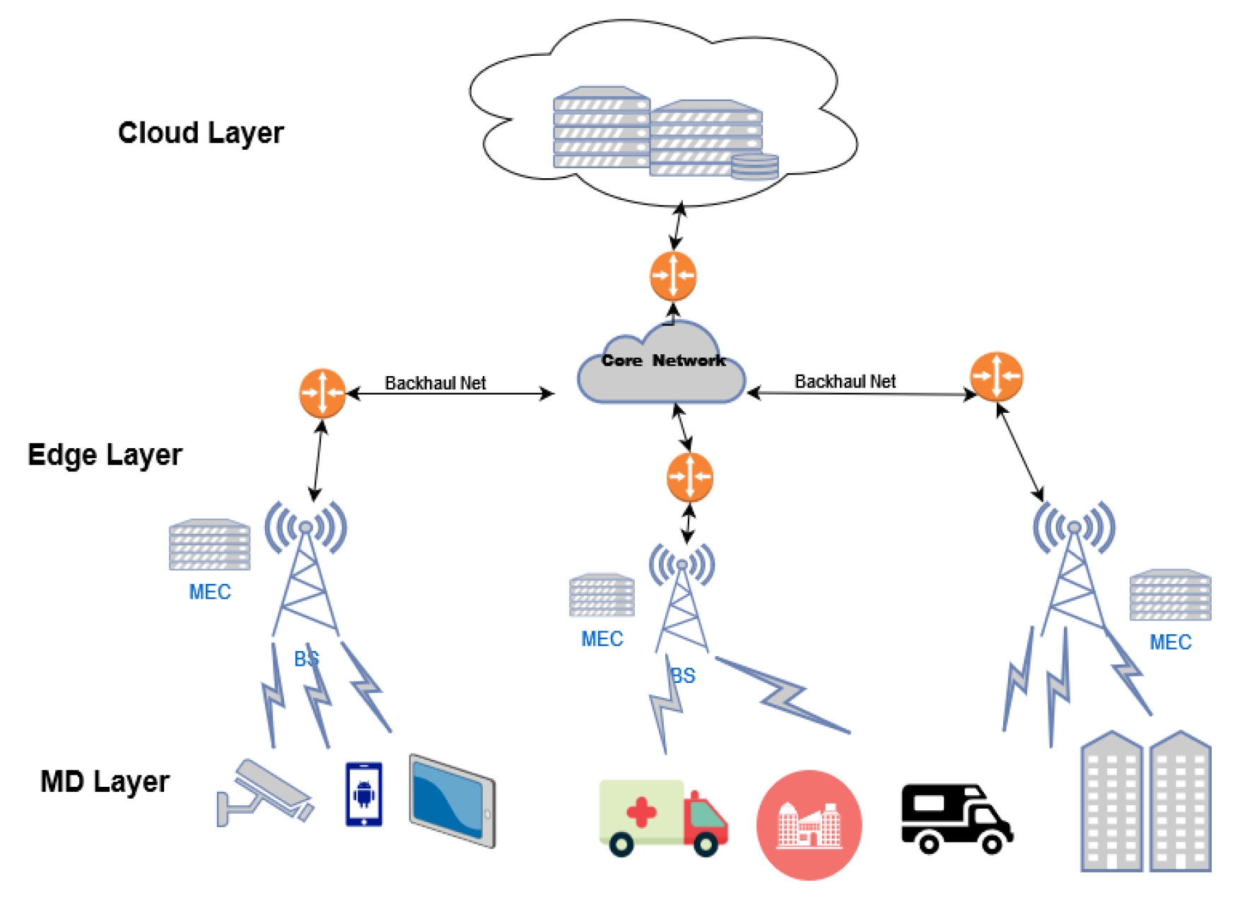
Figure 2.
Propose System Model.
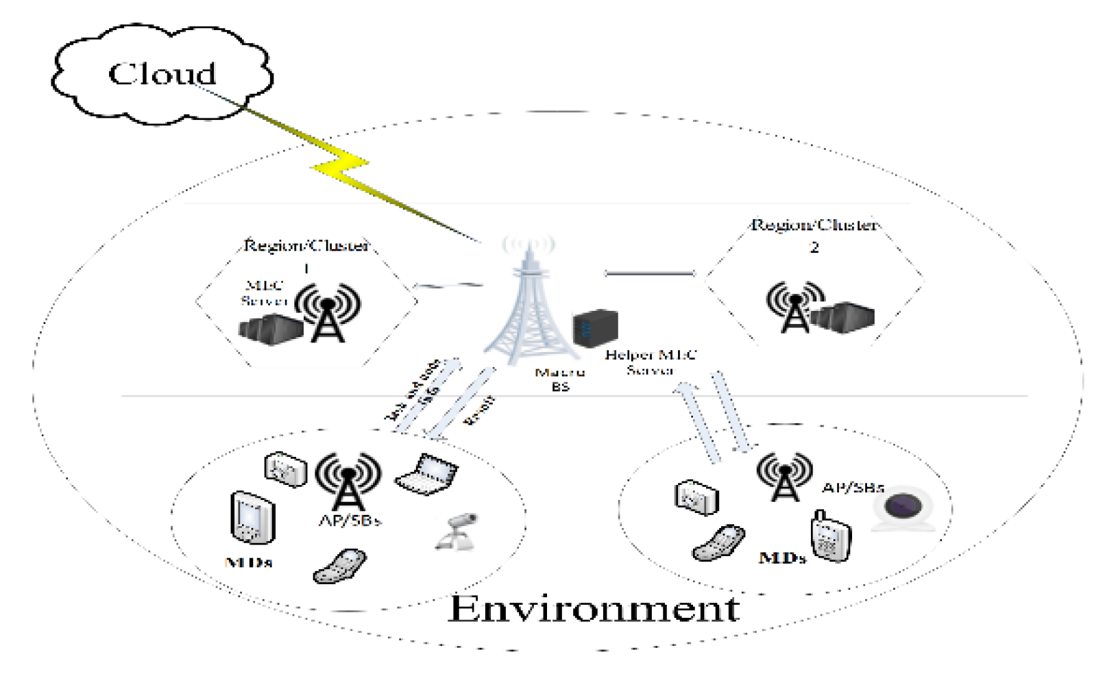
Figure 3.
work flow of BLSTM Prediction.
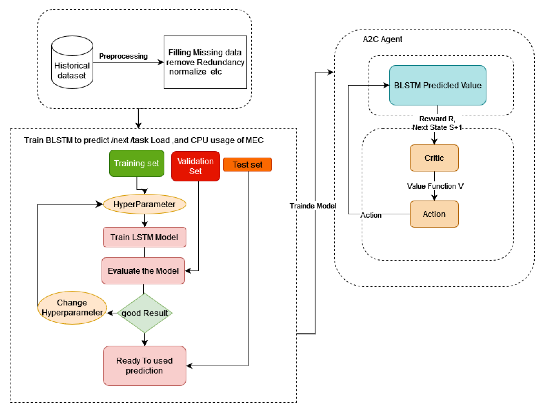
Figure 5.
Model Loss MAE and MSE.
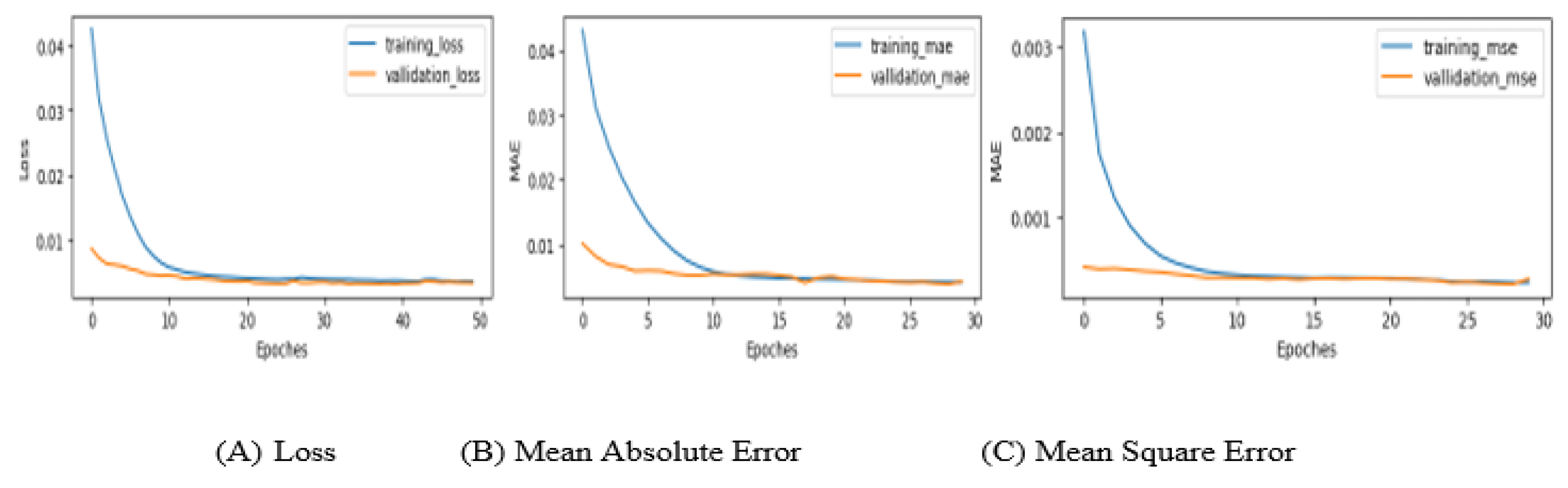
Figure 6.
prediction of Requested of memory and CPU against time in(s).
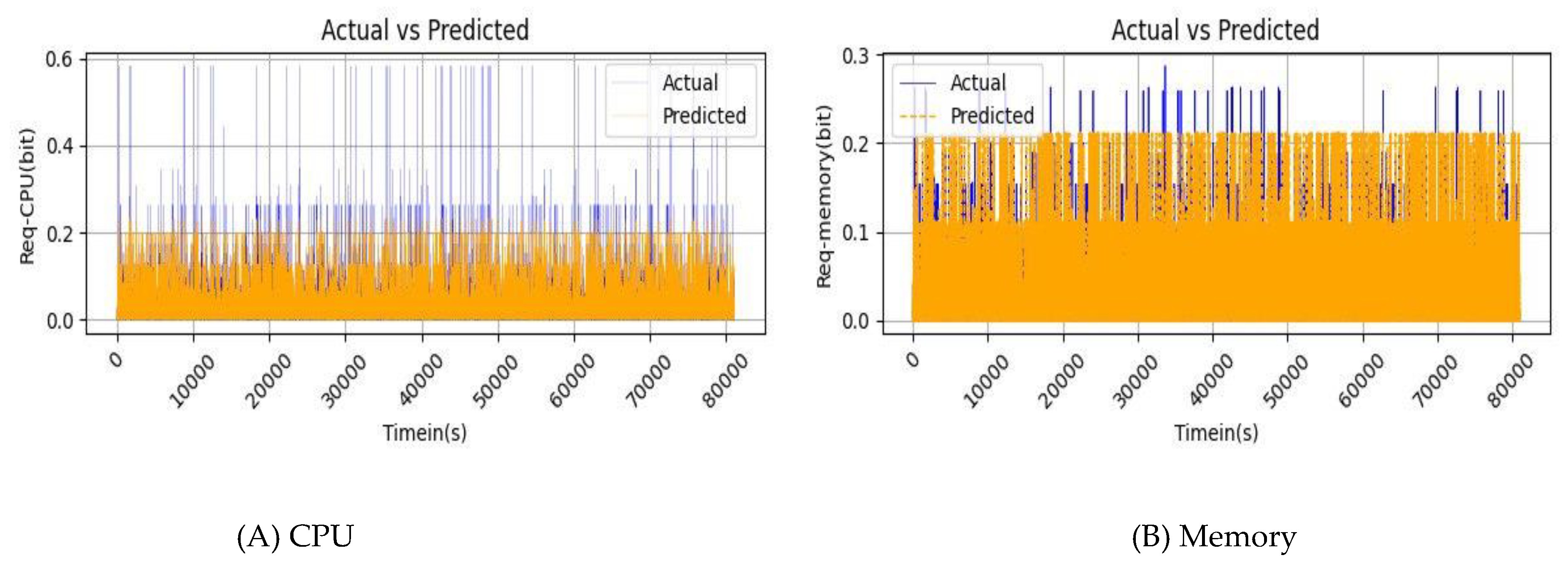
Figure 7.
Performance evaluation under different no of Task in time slot.
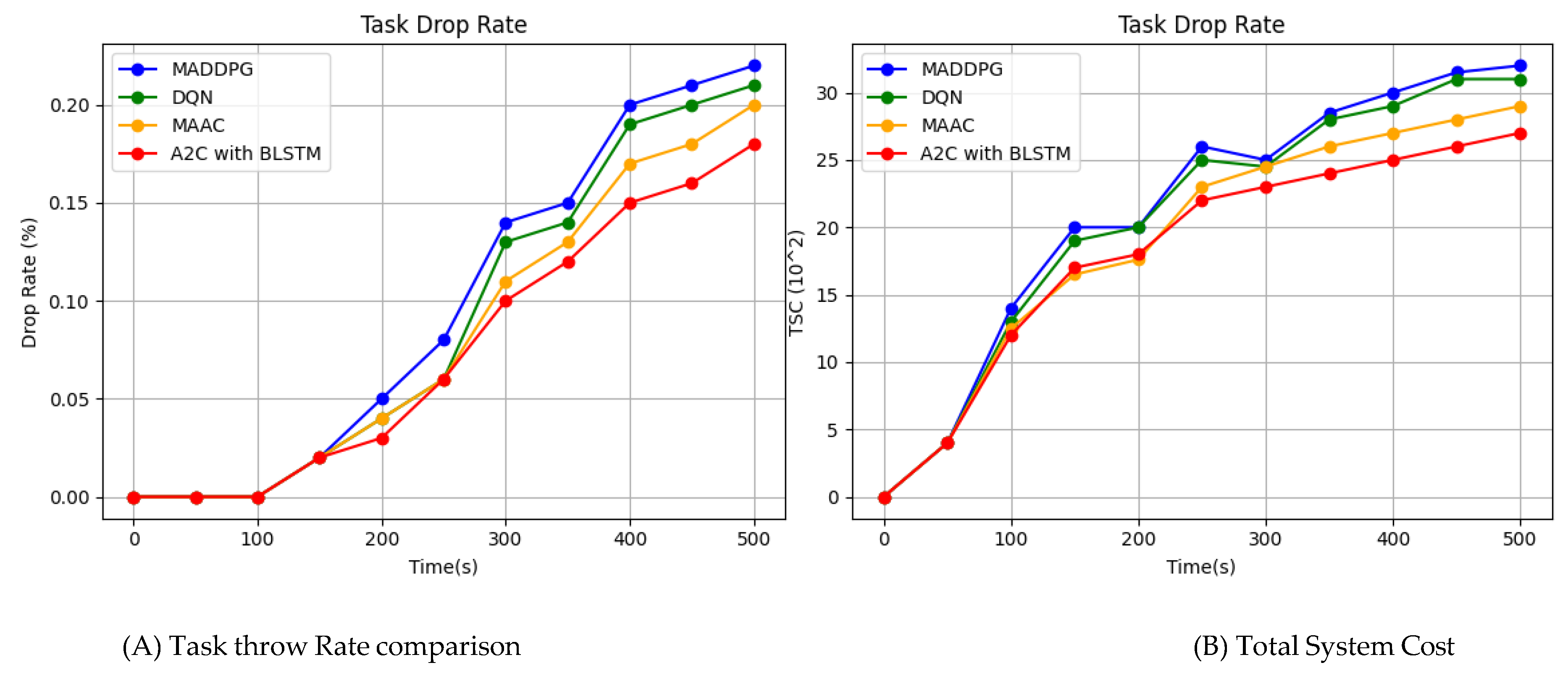
Figure 8.
Performance evaluation under different max tolerance latency (in seconds)
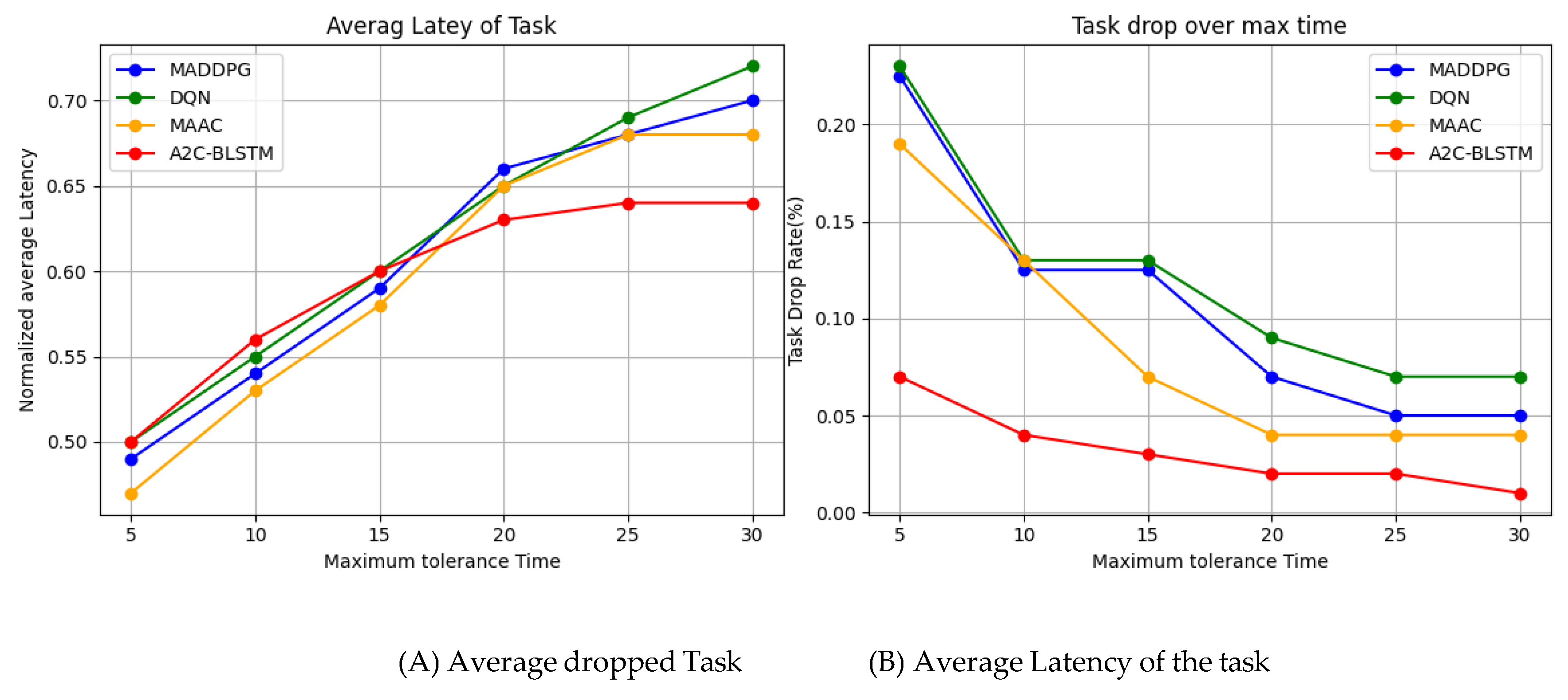
Figure 9.
Diagram of real-time simulated decision results.
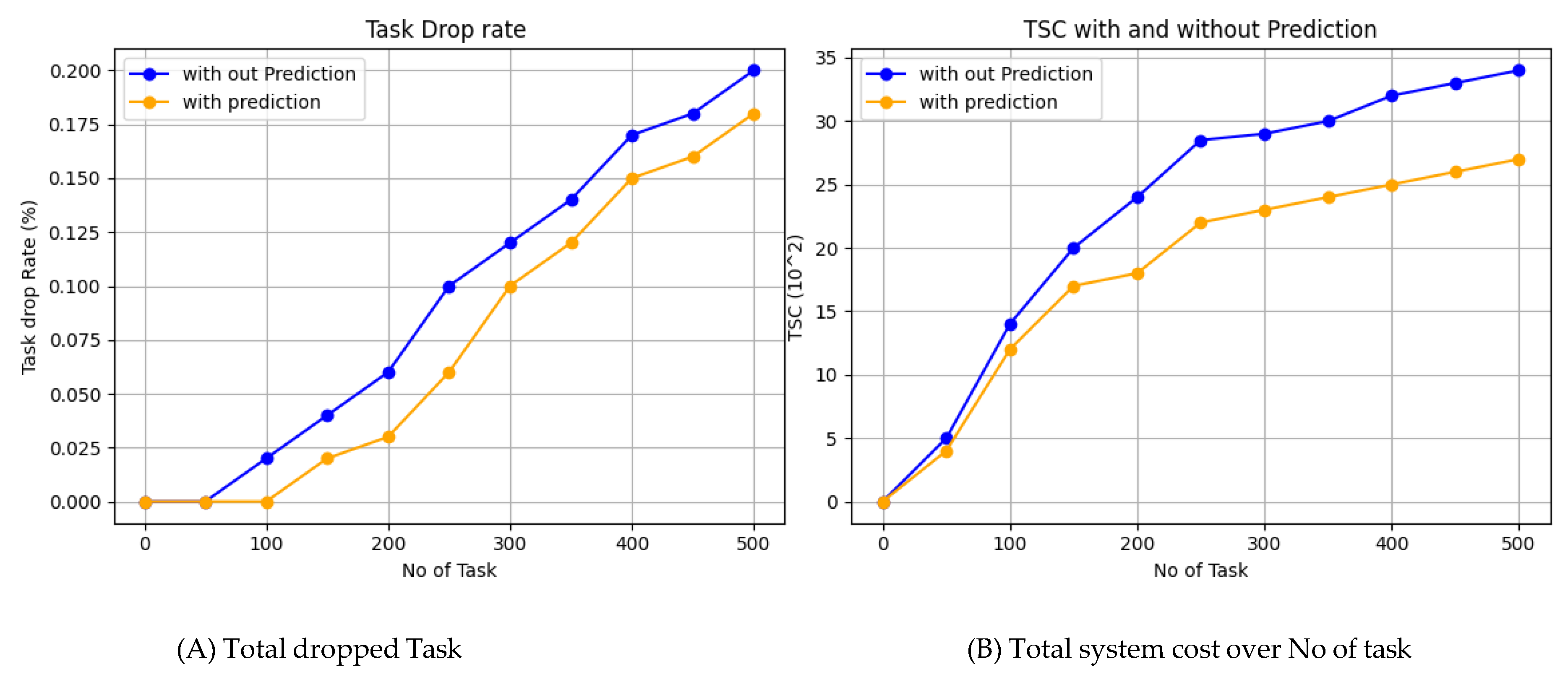

Table 1.
Summary Of Notation.
| Notation | Definition |
|---|---|
| c | Represents the cost of task consumed energy and delay. |
| α, β | The trade-off weight between energy and delay. |
| n | Represents the number of MD servers. |
| m | Represents the number of tasks. |
| Represents the CPU (computational resource) of the edge server. | |
| Represents the communication bandwidth. | |
| Represents the required size per bit for this type of task (in CPU cycles/bit). | |
| Represents the transmission rate of the input data to the MEC m. | |
| Represents the data size. | |
| Represents the CPU frequency of the MD (processing capacity (bits/s)). |
Table 2.
Simulation Parameter.
| Parameter | Value | Description |
|---|---|---|
| 10MHz | Bandwidth for offloading devices (MHz) | |
| 2.5GHz | Local CPU capacity (GHz/sec) | |
| 41.8GHz | MEC CPU capacity (GHz/sec) | |
| Energy consumption per CPU cycle | ||
| 1 | Gaussian channel noise | |
| 5w | Energy consumption per CPU cycle |
Disclaimer/Publisher’s Note: The statements, opinions and data contained in all publications are solely those of the individual author(s) and contributor(s) and not of MDPI and/or the editor(s). MDPI and/or the editor(s) disclaim responsibility for any injury to people or property resulting from any ideas, methods, instructions or products referred to in the content. |
© 2025 by the authors. Licensee MDPI, Basel, Switzerland. This article is an open access article distributed under the terms and conditions of the Creative Commons Attribution (CC BY) license (http://creativecommons.org/licenses/by/4.0/).
Copyright: This open access article is published under a Creative Commons CC BY 4.0 license, which permit the free download, distribution, and reuse, provided that the author and preprint are cited in any reuse.


