
Submitted:
27 September 2025
Posted:
28 September 2025
You are already at the latest version
Abstract
Resource prediction in heterogeneous cloud environments is hard because of diverse node configurations, monitoring metrics, execution logs, and injected failures. Neural models can capture temporal patterns but miss sparse discrete features. Tree-based models can model categorical data but cannot handle complex spatio-temporal patterns. We propose MHST-GB, a Multi-Modal Hierarchical Spatio-Temporal Ensemble Network with Gradient Boosting Integration. The framework uses modality-specific neural encoders with correlation-guided attention for fusion. It combines a dual-path design of deep spatio-temporal networks and LightGBM for complementary feature spaces. It also adds a feedback-driven training method that adjusts attention weights based on feature importance. With curriculum learning, FMSE loss, Mixup, and DropConnect, MHST-GB gains robustness and generalization for accurate multi-resource prediction in heterogeneous cloud environments.
Keywords:
Multi-Modal Learning
; Spatio-Temporal Modeling
; ensemble learning
; LightGBM integration
; Cloud Resource Prediction
I. Introduction
Accurate prediction of multiple resource metrics is essential for scheduling, autoscaling and fault mitigation in heterogeneous cloud systems. Predictors must reconcile dense time-series signals, sparse categorical configuration data, and intermittent log events. Existing solutions split into two classes: sequence models (e.g., TCN, RNN) that capture temporal dependencies, and gradient boosting machines that handle tabular heterogeneity and categorical splits but lack native long-range temporal modeling.
Recent applied studies report that hybrid designs combining engineered statistical summaries with learned temporal embeddings reduce prediction variance under distribution shift and improve operator-level interpretability; these findings motivate explicit LightGBM feedback and correlation-guided fusion in our design.
This paper proposes MHST-GB, a multi-modal hierarchical spatio-temporal ensemble that jointly optimizes deep temporal representations and LightGBM predictions. Contributions are: (1) a dual-path architecture combining modality-specific neural encoders and LightGBM; (2) a correlation-guided attention mechanism with LightGBM-driven feedback; (3) a targeted training regime using focal MSE and curriculum scheduling; (4) empirical evaluation demonstrating consistent gains on standard metrics.
II. Related Work
Luo et al. [1] presented Gemini-GraphQA that combines language models and graph encoders. Their work shows how graph-aware design can improve reasoning and execution. Duc et al. [2] studied workload prediction in cloud-edge environments. They focused on proactive allocation of resources and showed the importance of prediction for large-scale systems.
Rondón-Cordero et al. [3] reviewed ensemble learning methods for energy consumption forecasting. They explained how ensemble models give better performance than single models but also discussed the cost of complexity. Bawa et al. [4] used ensemble methods for workload prediction in cloud systems. Their results showed higher accuracy and confirmed the advantage of model integration in cloud resource management.
Krishnan [5] examined AI methods for dynamic allocation and auto-scaling in cloud computing. The work showed that AI can improve efficiency but also needs careful design to avoid overhead. Sanjalawe et al. [6] gave a review of AI-based job scheduling. They covered different techniques and pointed out that scalability and fairness remain open problems.
Huang [7] proposed a framework for demand prediction using a mix of statistical analysis and neural models. This work showed that hybrid approaches can handle both continuous and discrete data in cloud systems. Sunder et al. [8] designed a hybrid deep learning model for smart building energy load forecasting. Their study proved that combining multiple neural architectures can capture complex spatio-temporal behavior.
Singh et al. [9] developed an ensemble-based system for water quality classification. They showed that ensemble methods can work well for heterogeneous data beyond cloud environments. Khoramnejad and Hossain [10] studied generative AI for optimization in wireless networks. Their survey described the use of generative models for resource allocation and pointed to challenges in integrating such systems with current network infrastructure.
III. Methodology
We propose MHST-GB, a hybrid model combining spatio-temporal deep networks with LightGBM for multi-resource prediction in heterogeneous cloud environments. Four modalities—configuration, monitoring, logs, and faults—are encoded via TCN, BiGRU, and CNN, then fused through attention and fed into LightGBM. This design captures temporal patterns and heterogeneous feature interactions efficiently. Curriculum learning, adaptive rates, and focal loss enhance performance. See Figure 1.
IV. Model Overview
MHST-GB jointly models heterogeneous, multi-modal, and irregular cloud workload data. Given M metrics and T time steps, we learn:
Here denotes the prediction for metric m at time t; denotes static node configuration features; , and denote monitoring, parsed task logs and fault streams over the input window respectively.
We adopt a dual-path design: deep encoders extract spatio-temporal features, while LightGBM models tabular sparsity and non-linear interactions.
A. Configuration Encoder
Static configuration is encoded via residual MLP:
In this equation ; and produce . Activation denotes ReLU in our implementation.
B. Monitoring Metric Encoder
Monitoring input is processed by TCN with dilated convolution:
Here K is kernel size, d the dilation factor, the convolutional kernel weights and the multivariate monitoring vector per time step. TCN outputs are projected to the shared embedding dimension d before fusion.
C. Task Event Sequence Encoder
Parsed task logs are passed into BiGRU:
The parser yields numeric descriptors per event; the BiGRU concatenates forward and backward hidden states and projects the result to for fusion.
D. Fault Injection Encoder
Fault logs are embedded and passed through a 1D-CNN:
Fault codes are mapped to trainable embeddings and convolved with temporal kernels; outputs are pooled and projected to .
E. Feature Alignment and Fusion
We use correlation-guided attention to align modalities, motivated by the fact that LightGBM feature importance metrics can identify strong predictors, which in turn inform attention weights. Let be the Pearson correlation between modality j’s output and the target:
In practice is computed on modality-level summaries over the training set; is a temperature hyperparameter tuned on validation. Each is linearly projected to common dimension d prior to weighting. These fused embeddings feed both the deep prediction head and the LightGBM learner, ensuring that modality weighting benefits both branches.
F. Prediction and Ensemble Integration
The fused vector enters a Multi-Head Self-Attention (MHSA) block to model inter-metric dependencies:
Where are linear projections of and denotes key dimension; softmax is applied over the key axis. The MHSA output is processed by a regression MLP to produce . Simultaneously, and selected engineered features are input to LightGBM to produce . The final prediction is:
The scalar is selected on the validation set (grid search) or learned as a small parameter. Both branch outputs are in before fusion. This fusion capitalizes on LightGBM’s ability to capture decision boundaries in sparse feature spaces, complementing deep learning’s high-capacity nonlinear modeling.
G. Loss Function and Training Strategies
We employ a Focal Mean Squared Error (FMSE) to emphasize harder samples:
Here (>0) controls focal emphasis; is the per-metric empirical standard deviation computed on the training set (epsilon added if zero). Training incorporates:
- Curriculum Learning: early training uses shorter sequences for stability.
- Layer-wise Adaptive Learning Rate (LALR): .
- LightGBM Feature Importance Feedback: periodic feature importance analysis informs neural attention re-weighting.
By embedding LightGBM into every modality’s feature flow rather than as a post-hoc baseline, the model exploits both structured learning and deep representation learning in a single, unified pipeline. Figure 2 illustrates the comprehensive training strategy employed in our framework.
V. Feature Engineering and Preprocessing Enhancements
Effective feature preparation is critical for the MHST-GB framework, as the data exhibits heterogeneity, temporal irregularity, and varying levels of sparsity. We design the feature pipeline to simultaneously serve deep neural encoders and LightGBM, ensuring that both branches receive modality-specific yet complementary inputs are shown in Figure 3
A. Correlation-Guided Feature Selection
To mitigate redundant features post-encoding, we compute Pearson correlation with respect to target y:
Features with are pruned. Threshold τ is tuned via cross-validation. This improves LightGBM split quality and regularizes neural branches.
B. Temporal Aggregation and Statistical Summarization
To handle variable-length sequences, we apply aggregations (mean, variance, max, EMA):
Aggregated features go to LightGBM; full sequences feed neural encoders, ensuring multi-resolution representation.
C. Log-Parsing-Based Numeric Extraction
Task commands are parsed via into numerical vectors:
These features reduce noise and enhance semantic consistency for both LightGBM and neural paths.
VI. Additional Optimization Strategies
Beyond architectural design and feature processing, we incorporate training and inference optimizations to maximize predictive performance while ensuring stability and interpretability are shown in Figure 4
A. Curriculum-Based Multi-Stage Training
Instead of training the entire network on full-length sequences from the start, we employ curriculum learning. Let be the initial sequence length, and at each stage s, we increase it to . This allows encoders to first learn stable local dependencies before modeling long-range temporal patterns, improving convergence stability.
B. LightGBM Feature Importance Feedback Loop
During training, LightGBM produces a gain-based importance score for each feature f. We normalize these scores and use them to adjust the attention weights in the neural fusion layer:
where is the average importance of features from modality j, and controls the contribution of LightGBM feedback. This cross-model synergy improves alignment between decision boundaries and learned embeddings.
C. Regularization via Mixup and DropConnect
To improve robustness, we apply temporal mixup for sequence data:
where . Additionally, DropConnect is applied to fully connected layers in the deep branch, randomly dropping weights rather than activations, encouraging redundancy and preventing co-adaptation.
These optimizations collectively ensure that MHST-GB not only captures complex temporal-spatial relationships but also retains the practical advantages of gradient boosting in handling mixed and sparse data representations.
VII. Evaluation Metrics
To assess MHST-GB, we adopt four standard metrics covering absolute/relative error and explanatory power:
Weighted Relative Error (WRE) is the main metric:
where denotes the metric weight.
Mean Absolute Error (MAE) measures overall error magnitude:
Root Mean Squared Error (RMSE) penalizes large deviations:
Coefficient of Determination () reflects explained variance:
Together, these metrics evaluate accuracy, robustness, and generalization.
VIII. Experiment Results
We compare MHST-GB against LSTM-Base, TCN-Attn, and LightGBM-Only. Table 1 and Figure 5 show MHST-GB achieves the best performance across all metrics.
Ablation results (Table 2) show LightGBM integration yields the largest single-component gain (WRE 0.137 without LightGBM vs 0.124 full). Removing correlation-guided attention or the feedback loop degrades performance, confirming that modality alignment and cross-model feedback contribute non-redundant improvements. Error diagnostics (attention heatmaps and GBM importance plots) indicate LightGBM captures threshold-like and sparse predictors while the neural branch reduces temporally structured residuals.
A. Ablation Study
We evaluate the effects of LightGBM, correlation-guided attention, and feedback loop. Table 2 confirms each component contributes, with LightGBM providing the largest benefit.
IX. Conclusion
We proposed the MHST-GB framework, a multi-modal hierarchical spatio-temporal deep ensemble with integrated LightGBM for predicting cloud resource monitoring metrics. By unifying modality-specific neural encoders, correlation-guided fusion, and gradient boosting’s structured feature modeling, our approach achieves superior accuracy and robustness over both neural-only and boosting-only baselines. Ablation results confirm the complementary nature of deep representation learning and decision tree-based modeling in complex cloud workload prediction tasks.
MHST-GB assumes adequate historical coverage per node and representative fault injections; abrupt unobserved distribution shifts may require online GBM updates and domain adaptation. Future work will examine online LightGBM updating and formal calibration of the feedback coefficient under non-stationarity.
References
- Luo, X.; Wang, E.; Guo, Y. Gemini-GraphQA: Integrating Language Models and Graph Encoders for Executable Graph Reasoning. Preprints 2025. [Google Scholar] [CrossRef]
- Duc, T.L.; Nguyen, C.; Östberg, P.O. Workload Prediction for Proactive Resource Allocation in Large-Scale Cloud-Edge Applications. Electronics 2025, 14, 3333. [Google Scholar]
- Rondón-Cordero, V.H.; Montuori, L.; Alcázar-Ortega, M.; Siano, P. Advancements in hybrid and ensemble ML models for energy consumption forecasting: results and challenges of their applications. Renewable and Sustainable Energy Reviews 2025, 224, 116095. [Google Scholar] [CrossRef]
- Bawa, J.; Kaur Chahal, K.; Kaur, K. Improving cloud resource management: an ensemble learning approach for workload prediction: J. Bawa et al. The Journal of Supercomputing 2025, 81, 1138. [Google Scholar] [CrossRef]
- Krishnan, G. ENHANCING CLOUD COMPUTING PERFORMANCE THROUGH AI-DRIVEN DYNAMIC RESOURCE ALLOCATION AND AUTO-SCALING STRATEGIES. International Journal of Advanced Research in Cloud Computing 2025, 6, 1–6. [Google Scholar]
- Sanjalawe, Y.; Al-E’mari, S.; Fraihat, S.; Makhadmeh, S. AI-driven job scheduling in cloud computing: a comprehensive review. Artificial Intelligence Review 2025, 58, 197. [Google Scholar] [CrossRef]
- Huang, J. Resource Demand Prediction and Optimization Based on Time Series Analysis in Cloud Computing Platform. Journal of Computer, Signal, and System Research 2025, 2, 1–7. [Google Scholar]
- Sunder, R.; R, S.; Paul, V.; Punia, S.K.; Konduri, B.; Nabilal, K.V.; Lilhore, U.K.; Lohani, T.K.; Ghith, E.; Tlija, M. An advanced hybrid deep learning model for accurate energy load prediction in smart building. Energy Exploration & Exploitation 2024, 42, 2241–2269. [Google Scholar] [CrossRef]
- Singh, P.; Hasija, T.; Bharany, S.; Naeem, H.N.T.; Rao, B.C.; Hussen, S.; Rehman, A.U. An ensemble-driven machine learning framework for enhanced water quality classification. Discover Sustainability 2025, 6, 552. [Google Scholar] [CrossRef]
- Khoramnejad, F.; Hossain, E. Generative AI for the optimization of next-generation wireless networks: Basics, state-of-the-art, and open challenges. IEEE Communications Surveys & Tutorials 2025.
Figure 1.
Overall architecture of the Multi-Modal Hierarchical Spatio-Temporal Ensemble Network with Gradient Boosting Integration (MHST-GB). The model processes four input modalities through specialized encoders: Residual MLP for configuration data, TCN for monitoring metrics, BiGRU for task sequences, and 1D-CNN for fault injection records. Features are aligned using correlation-guided attention fusion before dual-path processing through MHSA and LightGBM, culminating in a weighted ensemble prediction optimized with Focal MSE loss.
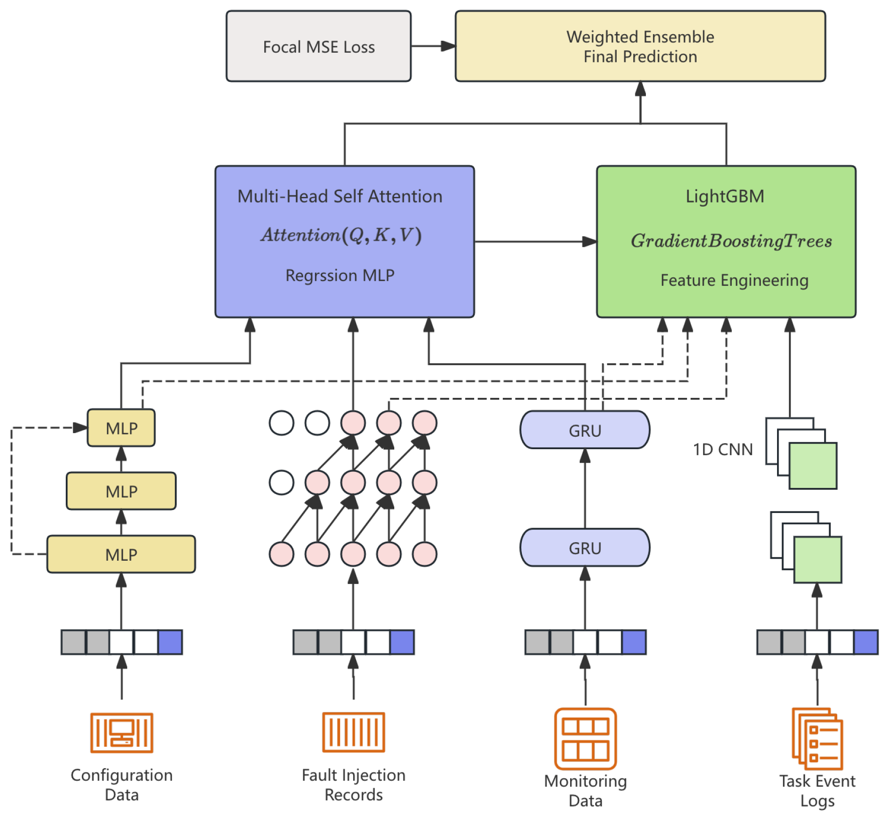
Figure 2.
Training strategies and optimization dynamics.
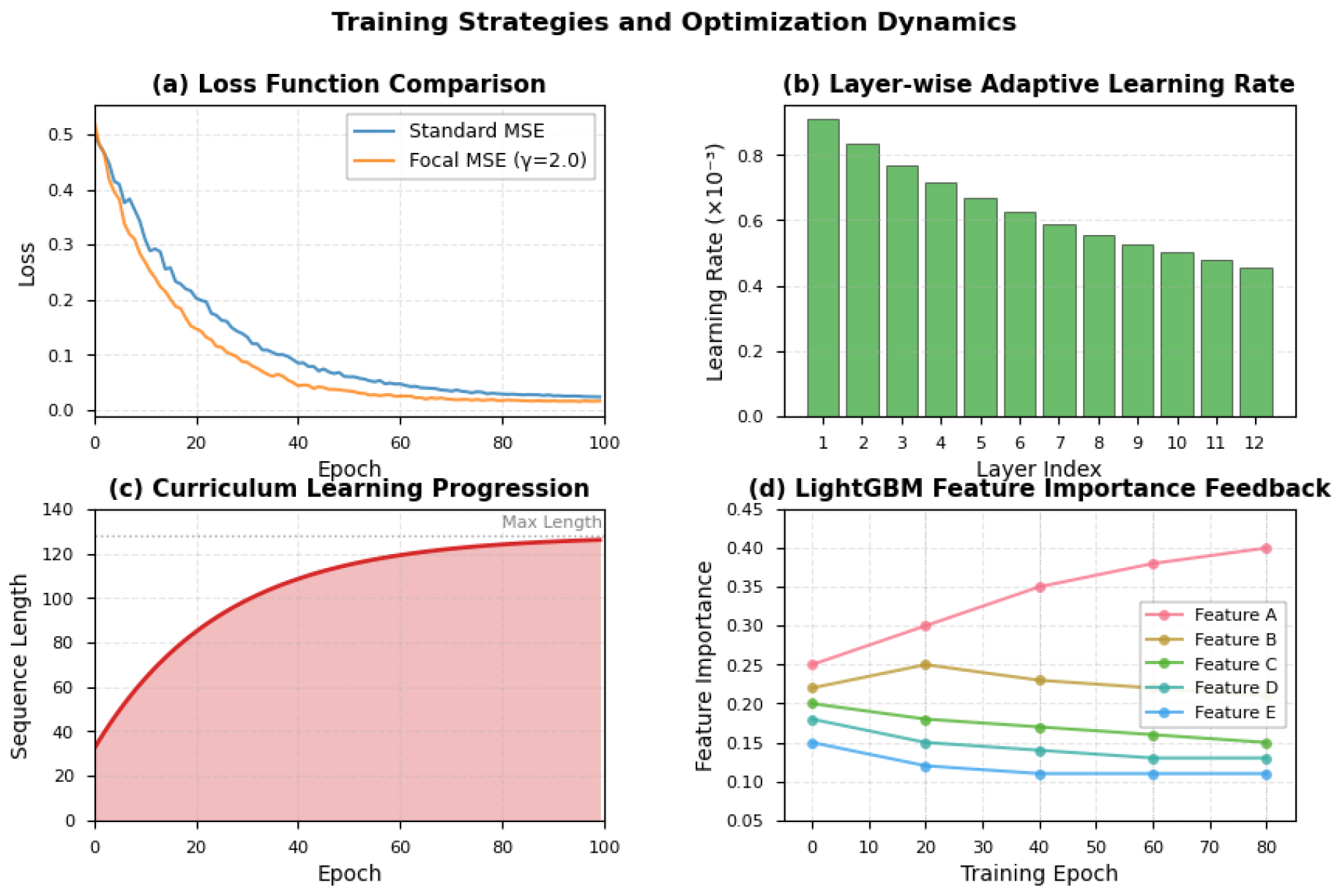
Figure 3.
Feature engineering and preprocessing pipeline. The three-stage process includes correlation-guided feature selection with threshold determined via cross-validation, temporal aggregation using statistical functions and exponential moving average (EMA), and log-parsing-based numeric extraction through template mining . The pipeline produces both fine-grained features for the neural branch and coarse-grained statistical summaries for LightGBM.
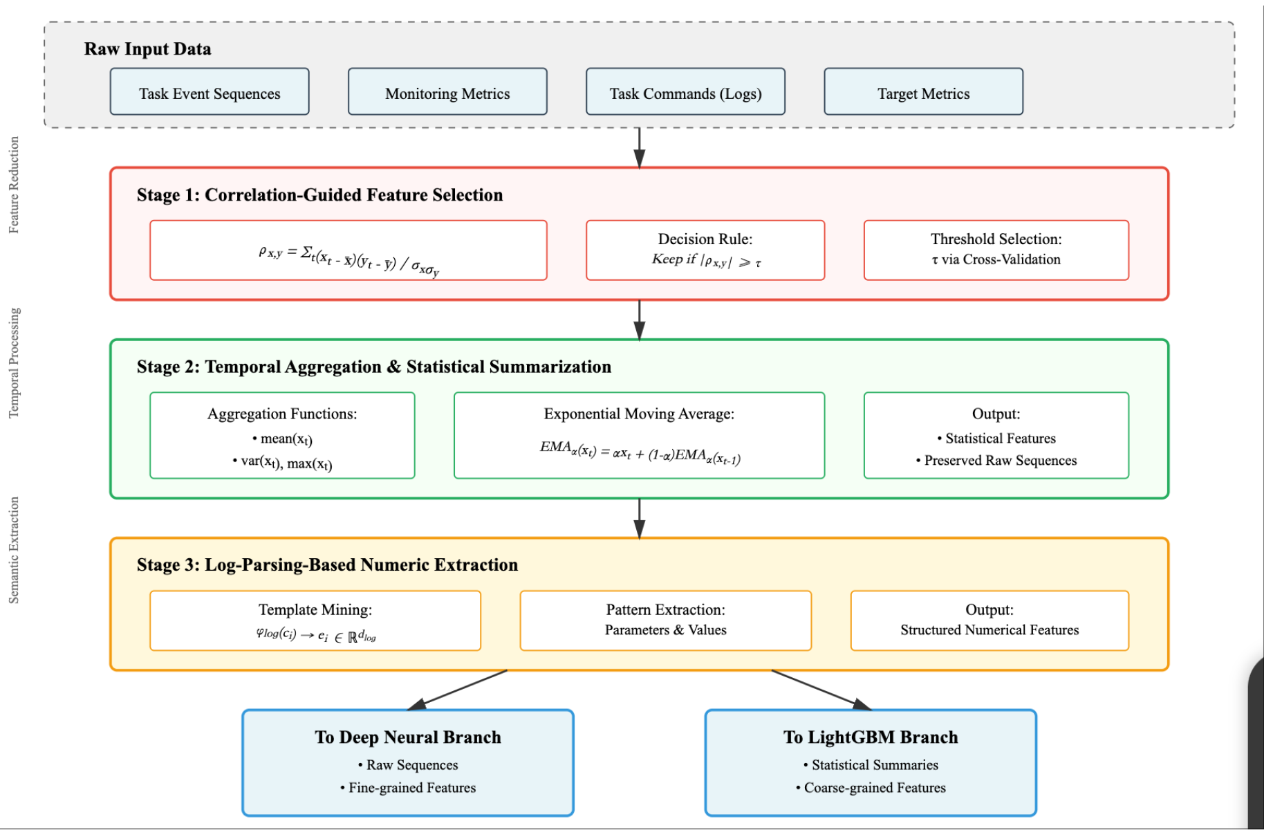
Figure 4.
Multi-stage training and optimization strategies employed in MHST-GB. The framework combines curriculum-based training with progressive sequence length increase (), LightGBM-neural feedback loop for adaptive attention weight adjustment, and regularization techniques including temporal mixup and DropConnect. These strategies collectively ensure stable convergence and improved generalization performance..
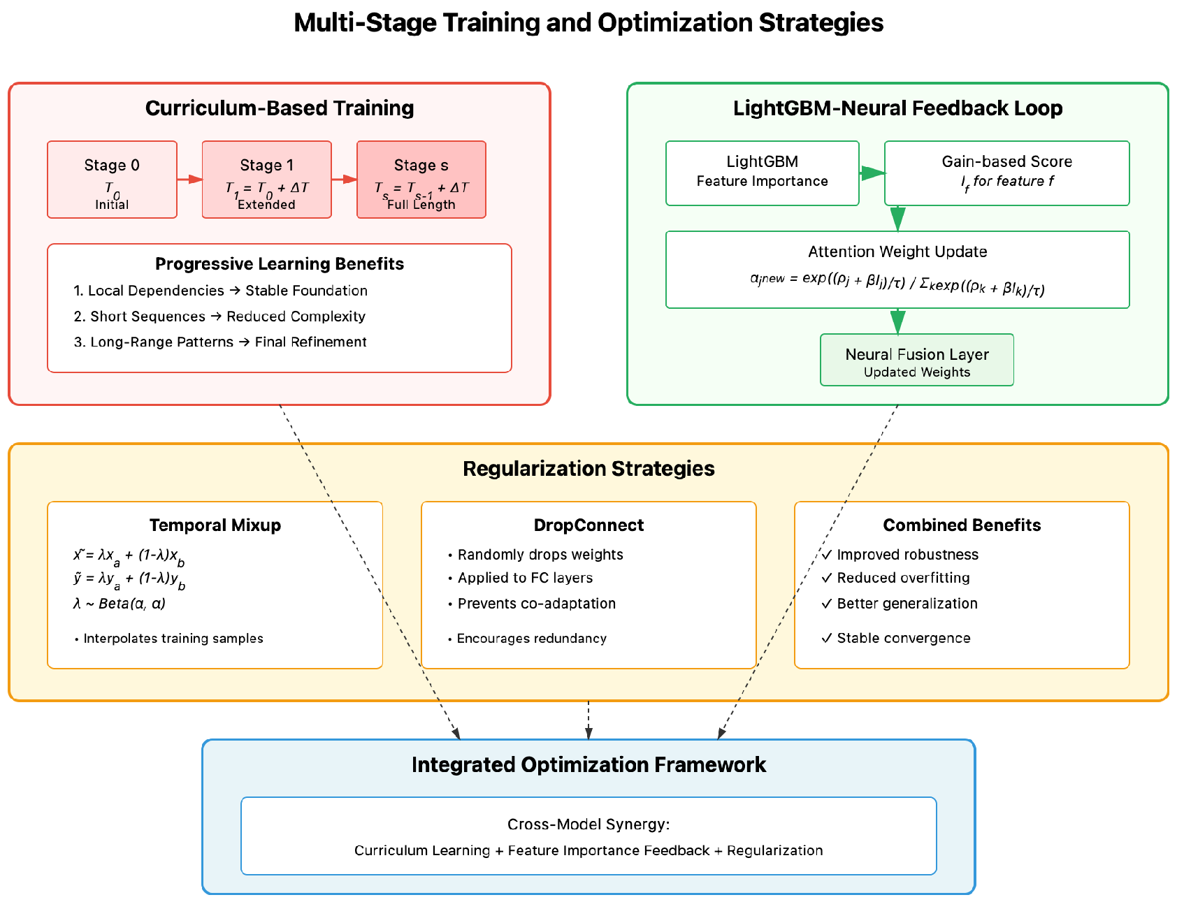
Figure 5.
Model indicator change chart.
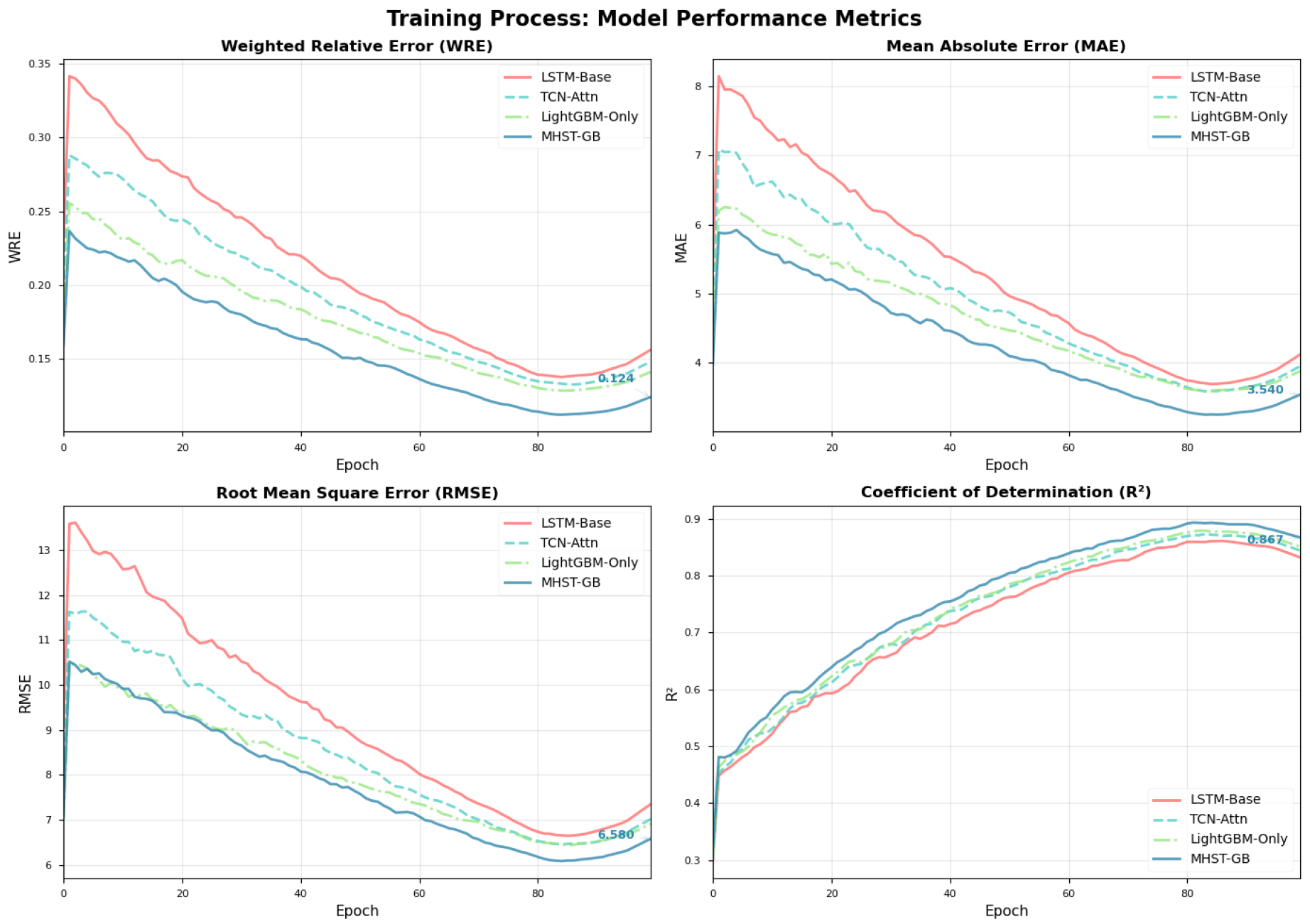

Table 1.
Performance comparison on the test set. Best results in bold.
| Model | WRE | MAE | RMSE | |
|---|---|---|---|---|
| LSTM-Base | 0.156 | 4.12 | 7.35 | 0.832 |
| TCN-Attn | 0.148 | 3.95 | 7.02 | 0.844 |
| LightGBM-Only | 0.141 | 3.88 | 6.91 | 0.851 |
| MHST-GB (Ours) | 0.124 | 3.54 | 6.58 | 0.867 |
Table 2.
Ablation study results for MHST-GB.
| Variant | WRE | MAE | RMSE | |
|---|---|---|---|---|
| Full MHST-GB | 0.124 | 3.54 | 6.58 | 0.867 |
| w/o LightGBM | 0.137 | 3.78 | 6.84 | 0.854 |
| w/o Corr-Attn | 0.132 | 3.69 | 6.73 | 0.859 |
| w/o Feedback Loop | 0.129 | 3.61 | 6.65 | 0.863 |
Disclaimer/Publisher’s Note: The statements, opinions and data contained in all publications are solely those of the individual author(s) and contributor(s) and not of MDPI and/or the editor(s). MDPI and/or the editor(s) disclaim responsibility for any injury to people or property resulting from any ideas, methods, instructions or products referred to in the content. |
© 2025 by the authors. Licensee MDPI, Basel, Switzerland. This article is an open access article distributed under the terms and conditions of the Creative Commons Attribution (CC BY) license (http://creativecommons.org/licenses/by/4.0/).
Copyright: This open access article is published under a Creative Commons CC BY 4.0 license, which permit the free download, distribution, and reuse, provided that the author and preprint are cited in any reuse.


